Radial alignment of elliptical galaxies by the tidal force of a cluster of galaxies
Abstract
Unlike the random radial orientation distribution of field elliptical galaxies, galaxies in a cluster are expected to point preferentially towards the center of the cluster, as a result of the cluster’s tidal force on its member galaxies. In this work an analytic model is formulated to simulate this effect. The deformation time scale of a galaxy in a cluster is usually much shorter than the time scale of change of the tidal force; the dynamical process of the tidal interaction within the galaxy can thus be ignored. An equilibrium shape of a galaxy is then assumed to be the surface of equipotential, which is the sum of the self-gravitational potential of the galaxy and the tidal potential of the cluster at this location. We use a Monte-Carlo method to calculate the radial orientation distribution of these galaxies, by assuming the NFW mass profile of the cluster and the initial ellipticity of field galaxies. The radial angles show a single peak distribution centered at zero. The Monte-Carlo simulations also show that a shift of the reference center from the real cluster center weakens the anisotropy of the radial angle distribution. Therefore, the expected radial alignment cannot be revealed if the distribution of spatial position angle is used instead of that of radial angle. The observed radial orientations of elliptical galaxies in cluster Abell 2744 are consistent with the simulated distribution.
Keywords:
galaxies: clusters: general – galaxies: clusters: individual: Abell 2744 – galaxies: kinematics and dynamics – galaxies: structure.1 Introduction
The total mass of a cluster of galaxies is dominated by dark matter, which couples only through gravity with ordinary matter. Therefore, to map the density profile of a cluster, one needs to find how luminous matter in a cluster is related to its gravitational potential. Each way of doing so leads to a method of cluster mass mapping. Assuming some sort of dynamical balance established, one can model how the spatial distribution and velocity dispersion of galaxies respond to its gravitational potential and then develop a technique to determine the mass distribution (Carlberg et al., 1997; Kent & Gunn, 1982). Hydrostatic equilibrium supposed, the density and temperature profiles of hot gas are related to the shape of the gravitational potential well (Fabricant et al., 1980; Xue & Wu, 2002). Finding the manner of light rays bent by gravity gives birth to the method of gravitational lensing (Kaiser & Squires, 1993; Umetsu & Broadhurst, 2008). Although many approaches have been made, the results from those are not always in good agreement (Wu et al., 1998; Bartelmann & Steinmetz, 1996). Therefore, it is still useful to find other independent probes.
An extended object in a non-uniform gravitational field feels a distorting tidal force. The tidal force from the mass of a cluster can change the shape of its galaxies in a way that the radial orientation angles (see the upper panel of Fig. 1 for an illustration) of elliptical galaxies in a cluster show an anisotropic distribution toward the cluster center different from the isotropic distribution of field galaxies; this phenomenon is referred to as radial alignment (RA). If RA really exists and is caused by the tidal effect of the cluster mass, then a new link between an observable, i.e. the radial angle distribution (RAD) of elliptical galaxies, and the gravitational potential of the cluster can be found.
The idea that the cluster tidal force can cause RA was first proposed by Thompson (Thompson, 1976), in order to explain “a possible indication that the galaxies are preferentially aligned along the radius vector to the center of the cluster” for the Coma cluster (Hawley & Peebles, 1975). In recent years, more observational evidence has been found to support this idea (Pereira & Kuhn, 2005; Agustsson & Brainerd, 2006; Faltenbacher et al., 2007). Theoretically, Ciotti & Dutta (1994) studied the dynamical process of shape changing of an elliptical galaxy under the cluster’s tidal field using N-body simulations, and showed an alignment tendency between the galaxies’ major axes with the radial direction. Pereira et al. (2008) found strong RA of dark matter substructures in a cluster halo in N-body simulations. Usami & Fujimoto (1997) studied a gaseous ellipsoid of uniform density orbiting in the logarithmic potential, and discussed the application of their result to the alignment of galaxies in rich clusters. They concluded that inside a critical radius, galaxies would be disrupted by the tidal force of the cluster, whereas beyond the critical radius the major axes of elliptical galaxies are locked in radial direction. None of the previous works take the intrinsic ellipticity distribution of galaxies into consideration. In Usami & Fujimoto (1997) all elliptical galaxies’ intrinsic shape were set spherical, unlikely in real cases. In our work, the ellipticity distribution of field elliptical galaxies, which can be thought unaffected by environment, is used as the intrinsic ellipticity distribution.
This work aims to formulating an analytic model to simulate RA quantitatively. Section 1 is to verify qualitatively that the shape changing timescale for most galaxies in a cluster is short enough compared with the Keplerian motion period so that we can ignore the dynamical process of tidal distortion and assume an equilibrium shape of the galaxy. In section 2 we calculate the equilibrium shape of an elliptical galaxy analytically. Then the projection effects are included and RAD is generated by a Monte-Carlo method. Finally the observed RADs of the clusters Abell 2744 are compared.
2 Qualitative discussion
Consider a galaxy in a cluster, and the vector from the galaxy center to the cluster center is . The enclosed mass within radius is denoted by and its potential field is . The tidal force acting on a mass element of the galaxy is approximately
| (1) |
where and are the vectors from the mass element to the galaxy center and to the center of the cluster, respectively. denote the three cartesian coordinate components of a vector. The Einstein summation convention is used in this work. We define a tidal potential corresponding to the tidal force, which is
| (2) |
The mass distribution of the cluster is treated as spherically symmetric, so its gravity acting on a mass element can be written as
| (3) |
where denotes the enclosed mass in radius , and denotes the gravity potential caused by the mass gradient. Here since (Binney & Tremaine, 1987), we obtain
| (4) |
Substituting Equations (3) and (4) into Equation (2), and neglecting the variation of in small scale, we obtain
| (5) |
where is the component of along , and is the perpendicular component, which are illustrated in Fig. 1. Therefore the tidal force acting on an unit mass is obtained by .
An unit mass element is also subjected to the self-gravity from the galaxy,
| (6) | ||||
where and are the gravity acting on the unit mass from the luminous and dark matter at the effective radius of a galaxy; and are the mass and effective radius of the luminous matter in the galaxy. The luminous matter is assumed homogeneous, with density . is the enclosed mass of the dark matter within the effective radius. In this work, we only consider the tidal distorsion within the effective radius. The density profile of the dark matter in an elliptical galaxy is (Robles & Matos, 2012)
| (7) |
where is the central density, and is the scale radius. Therefore the dark mass enclosed within is . At the effective radius kpc, , , where is used. Therefore , , implying that the effect of the dark matter in an elliptical galaxy can be neglected within the effective radius. This has been comfirmed by de Paolis, Ingrosso & Strafella (1995), who found that dark matter inside the effective radius is negligible with respect to the luminous matter.


Define as the ratio of the tidal force and self-gravity,
| (8) |
which reflects the significance of tidal force compared with self-gravity. In the case of cluster A2744, the mass distribution can be modeled by a NFW profile with the parameter (Zhang et al., 2006). We take , i.e., the radius within which the mean density should be , as the boundary of the cluster, and set , the same order of magnitude as the average density of the Milky Way. We find that the galaxies with only compose 0.1% the volume of the cluster. Thus for a rich cluster like A2744, the condition is satisfied for most galaxies, which means that the tidal force is weak compared with the self-gravity of these galaxies.
Carter & Luminet (1983) calculated the response of a star under the tidal force which is weak compared with its self-gravity. Analogous to a star, a galaxy will have a trace-free quadrupole oscillation, with a frequency . Therefore the deformation time scale of a galaxy should be . Equation (8) is used to substituting , we obtain , where is the Keplerian time scale characterizing the rate of change of the tidal force. Since , we have . It follows that the galaxy will remain close to the stationary equilibrium state determined by the instantaneous value of the tidal potential (Carter & Luminet, 1983), where the equilibrium shape of the galaxy will coincide with the iso-potential surface of the equilibrium state .
3 Quantitative calculation of the effect of tidal force on RAD of galaxies in a cluster
3.1 Coordinate system
Undoubtedly, an elliptical galaxy with a central luminous ellipsoid and dark matter halo component is a very complex entity, and therefore, we need to assume some necessary simplifications and assumptions in order to be able to study mathematically the deformation of such a complicated system under the tidal force from a cluster. Since we only consider the tidal distorsion within the effective radius kpc, therefore hereafter the effect of dark matter is neglected (see section 2 for details). We assume that the surface of the luminous matter is an oblate ellipsoid (Lambas et al., 1992) at the effective radius, with ellipticity before tidal distortion, the equation of the shape can be written as,
| (9) |
where , and axes are the principal axes of the ellipsoid, and and are related by the following equation,
| (10) |
We require that the vector pointing to the center of the cluster falls in the plane , thus the coordinate system can be uniquely defined, as long as the center of the cluster is not on the axis.
The direction of the cluster center is denoted as:
| (11) |
where is the angle between the direction of the cluster center and the axis. The coordinate system and vector are illustrated in the lower panel of Fig. 1.
3.2 Deformation of a single elliptical galaxy
In order to simplify the calculation, according to the homoeoid theorem (Binney & Tremaine, 1987), we assume that the iso-potential surface of the gravity potential of the luminous matter at the effective radius coincides with the local surface of the luminous ellipsoid. Then the self-gravity potential of an elliptical galaxy at the effective radius before tidal distortion can be written as,
| (12) |
where . It is easy to find .
The contribution of tidal force is equivalent to adding a tidal potential upon the self-gravity potential ; here we take,
| (13) |
A little calculation gives,
| (14) |
where . Hence an explicit expression of is given by:
| (15) |
where , , , and . Therefore, the final shape of the distorted galaxy is fully described, given the initial , , , together with the cluster mass profile , which is taken as the NFW profile (Navarro et al., 1996),
| (16) |
where and the “scale radius” are parameters of the distribution. Define , where is the critical density defined as , where is the Hubble constant and is the gravitational constant,
| (17) |
where is the so-called “concentration parameter” defined as , where is the radius within which the mean density should be (Navarro et al., 1996). Substituting Equation (16) into the expression of , we get
| (18) |
where is the dimensionless radius. Given and , can be obtained from Equations (17) and (18). Analogously, , and all the parameters from to of the ellipsoid can be calculated.
3.3 Projection effects
From the view of an observer, the ellipsoidal shape of a galaxy is projected to become an ellipse. The next step is to determine the major axis of the projected ellipse and evaluate the angle between that and the direction toward the cluster center. The observer is assumed in the direction , which can be expressed as,
| (19) |
The problem is then reduced to such a constrained extremum value problem: To find the farthest point from the vector in the surface of
| (20) |
then the projection of on the celestial sphere, , is the direction of the major axis. Define as the projection of vector on the celestial sphere, we obtain the radial orientation angle as,
| (21) |
The details of solving the constrained extremum value problem are presented in the Appendix.
3.4 RAD of elliptical galaxies
In order to derive RAD of elliptical galaxies in a cluster, we use Monte-Carlo simulations. In each run, a set of elliptical galaxies are generated, each of which is given a set of parameters sampled with certain probability distributions, as discussed below.

With given, each galaxy from the set results in a (). is used to simulate a cluster with high concentration like Abell 2744 (see section 4.1); note that is also the concentration of Coma cluster (Rines & Diaferio, 2006) where RA was found for the first time. The effective density of each galaxy is set to be times . In this run, 100,000 galaxies are generated, with an intrinsic ellipticity distribution in Fig. 2, which is the ellipticity distribution of field galaxies (Fasano & Vio, 1991). Here the ellipticity of a generated ellipsoid is defined as , where and are the major and minor axes of the ellipsoid, respectively. The dimensionless projected distance of galaxies are sampled with a probability inversely proportional to , from to , corresponding to an approximation to the projected galaxies number density distribution in Baier (1976). Under such parameters, the maximum value of is 0.0057, which is far smaller than unity. For each galaxy, the direction toward the cluster center and the direction toward the observer in the principal axes coordinate system are sampled with an isotropic probability, corresponding to an isotropic position distribution, which is assumed as the initial configuration of galaxies in the cluster.
Fig. 3 shows RADs for the different center offset distances , where is defined as the dimensionless offset distance, where is the distance between the real mass center of the cluster and the reference center used in observation. When , the upper-left panel in Fig. 3 shows a single peak. Therefore if the reference center is the real cluster center, the major axes of the elliptical galaxies tend to point to the cluster center, i.e., we can see obvious radial alignment of the elliptical galaxies. However if the reference center has an offset distance from the real cluster center, since the major axes tend to point to the real center rather than the reference center, two peaks are found in RADs. As the center deviation distance increases, the two peaks depart from each other farther with increasing . Then the two peaks merge at degrees as keeps increasing. Finally, RAD becomes uniform distribution if , and at this moment, radial angle distribution becomes position angle distribution.
We also plot the distorted ellipticity distribution of ellipsoids after the simulation in Fig. 2. The width of the ellipticity distribution is broadened about , where and are the full widths at the half maximum (FWHM) of the ellipticity distributions before and after the simulation, respectively; meanwhile, the ellipticity distribution is shifted to higher values compared with the intrinsic one.

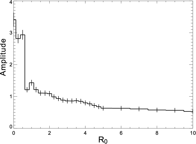
In order to further reveal the effect when the center of the cluster is mis-identified observationally, we define the “amplitude” of RAD as , where , and are the highest point, lowest point and mean value of RAD. intuitively suggests the significance that a peak-type distribution deviates from uniform distribution, i.e., when the distribution is similar to uniform distribution, while if there are significant peaks in the distribution. Fig. 4 shows as a function of the offset distance from the reference center to the true center of the cluster mass distribution. On the whole, decreases with increasing . For , a radial angle is equivalent to a position angle. The result in Fig. 4 explains why it is difficult to find RA with only the position angle distribution of elliptical galaxies in a cluster.
4 Observed RAD of Abell 2744
4.1 Selection of Elliptical Galaxies
Abell 2744 is one of the richest clusters of galaxies at intermediate redshift , known as a gravitational lens (Merten et al., 2011). Its parameters are estimated as (Zhang et al., 2006), (Demarco et al., 2003), hence the concentration parameter . Such a high mass concentration is expected to show some signature in its RAD. We thus choose this cluster to make the comparison with our theoretical work. The coordinate system is centered at , (Boschin et al., 2012). However, note that this cluster is an actively merging cluster (Owers et al., 2011); therefore, the cluster central position cannot be determined unambiguously (Zhang et al., 2006), which may bias RAD.
We retrieve HST (ACS/WFC) images in the F606W and F814W bands of two fields in the immediate vicinities of the cluster center (Date: 10/27/2009, PID: 11689, PI: Dupke). The associated images of A2744 are fully processed and drizzled. Photometry for objects is carried out using the Sextractor package (Bertin & Arnouts, 1996). The configuration parameters are listed in Table 1, and the magnitudes of the sources in the cluster are calibrated by the MAG_ZEROPOINT parameter in the AB system. The derived source catalogs in the two bands are matched to obtain 3005 true objects. The parameter Class/Star is used to get rid of stars, and then the removed stars are visually inspected in the images. The arcs and arclets, the spurious objects, the sources in the margins of images, and the sources inside other giant bright sources are visually identified and removed. The optical magnitudes of targets are corrected for the foreground extinction from the Galaxy according to the Schlegel-Finkbeiner-Davis Galactic reddening map (Schlafly & Finkbeiner, 2011).
| Parameters | Values |
|---|---|
| DETECT_MINAREA | 32 |
| DETECT_THRESH | 1.3 |
| DEBLEND_NTHRESH | 64 |
| DEBLEND_MINCONT | 0.005 |
| CLEAN_PARAM | 1.2 |
| BACK_SIZE | 40 |
| BACK_FILTERSIZE | 3 |
| BACKPHOTO_THICK | 24 |
Limited by the ACS field size, the measurement reaches out up to a distance of from the cluster center, which is about eight times of . These objects include both the foreground and background galaxies. In order to select the real cluster members, a color-magnitude diagram (CMD) is plotted in Fig. 5 using the magnitudes in the two filter bands, i.e., , . Since the colors of elliptical galaxies are redder than spiral galaxies (Baldry & Glazebrook, 2005), and the Butcher-Oemler condition is satisfied, i.e., the blue galaxies are those at least 0.2 mag bluer than the cluster ridgeline (Butcher & Oemler, 1984), a linear fitting, i.e.,
| (22) |
where , are the slope and intercept respectively, is applied to obtain the slope of the red sequence (Brow et al., 1992a, b) in the CMD, which is known as the collection of E/S0 galaxies. Here are obtained; therefore we select the E/S0 galaxies in the color range of . A faint end at about is used to divide the member elliptical galaxies from the background galaxies (Romano et al., 2010), which is approximately consistent with the rest-frame -band absolute magnitude of . Finally 199 elliptical galaxies are obtained. These selected elliptical galaxies are then visually inspected in the images.

4.2 RAD of Abell 2744
With SExtractor, we are able to quantitatively measure the orientations of the detected objects. We define the radial angle when the major axis of a projected ellipsoid points to the cluster center, and when the major axis orientates along the tangential direction. By separating the range of into 18 bins, we count the number of members in each bin. In order to obtain RAD with a high significance, we add together the number of galaxies in each bin of from the two filter bands. RAD of the all sources of Abell 2744, including the foreground and background galaxies, and RAD of the elliptical galaxies in Abell 2744 are presented in Fig. 6.

There are apparent tangential peaks centering at about in the upper panel of Fig. 6, which should be produced by gravitational lensing (Smail et al., 1997; Merten et al., 2011, e.g.), since the shapes of background galaxies are stretched tangentially after lensing (Joachim, 1997). Further more, since the selected elliptical galaxies are contaminated by some background galaxies, RAD in the bottom panel of Fig. 6 also show weak tangential peaks, which are fitted by a double-Gaussian component,
| (23) |
where is fixed. Additionally, a peak is located at close to , which is fitted by a Lorentzian component,
| (24) |
As a comparison, we also fit the central peak with a constant,
| (25) |
The two different fitting results are listed in Table 2. The relative error of is , suggesting that the central peak really exists, and thus the orientations of the elliptical galaxies are not random. -test is performed to obtain the probability that the model DG+L is better than the model DG+C. Given the value of , , where , and are the variances of the two models, respectively, thus we obtain .
| DG+L | ||||||
| 0.17(4.11) | 24(7) | -90(fixed) | 22(8) | 14.0/13 | ||
| DG+C | ||||||
| 4.5(0.6) | -90(fixed) | 6.8(9.5) | 27.8/15 |
5 Conclusion and Discussion
We estimated qualitatively the shape changing time scale of a galaxy in a cluster, which is found to be much shorter than its Keplerian time scale around the center of the cluster for most member galaxies. Thus we ignored the dynamical process of shape changing and assumed an equilibrium shape of galaxies. The shape of an elliptical galaxy under the tidal force of a cluster is calculated, by assuming that the density contour of the galaxy coincides with the equipotential surface of the sum of the tidal potential and self-gravitational potential of the galaxy. We then used the Monte-Carlo method to simulate RAD of galaxies in a cluster, taking the NFW mass profile of the cluster and the initial ellipticity distribution as that of field galaxies. The Monte-Carlo simulations also find that the elliptical galaxies in a cluster tend to be radially aligned if the real physical center is chosen as the reference center. If the reference center has an offset distance from the real center, then the farther the reference point away from the cluster center, the weaker the anisotropy of RAD will be shown. Therefore in order to find significant RA, the reference center should be set to the real physical center of the cluster. In addition, the distribution of position angles which is equivalent to cannot reflect RA. The observed RAD of cluster Abell 2744 is presented, using the data from HST. Comparing the observed RADs in Fig. 6 with the simulated ones in Fig. 3, we conclude that the observed non-uniform RADs are due to the tidal effects of these clusters.
In our model, the gravitational interaction between two nearby galaxies is neglected. We treated the galaxies as if they were moving under a smooth averaged field. In fact when two galaxies get close, the tidal effects from the nearby galaxy will weight over the entire cluster. This will increase the randomness of RAD of the whole cluster, because encounter events are random and the effects are local. The non-spherical symmetry and substructures of the cluster are also not included, since we applied the isotropic NFW mass profile. Those effects will be included in our following works. Our simulations place galaxies in the region where the self-gravity of the galaxies are far greater than the tidal force from the cluster, so tidal disruption of galaxies has not been taken into consideration.
In section 2, we assumed that a galaxy has a trace-free quadrupole oscillation under the weak tidal distorsion like a star (Carter & Luminet, 1983) with a period Gyr. However, an elliptical galaxy is a stellar system rather than a fluid system, and the oscillation can be quickly damped by Landau damping (Binney & Tremaine, 1987; Weinberg, 1994). Therefore, the time needed from the beginning of deformation to finally settling on the equilibrium state is indeed the damping time scale , if . In a finite stellar system like an elliptical galaxy, the time scale of damping the quadrupole oscillation (Weinberg, 1994, mode) is shorter than (see Weinberg (1994) for details). Therefore an elliptical galaxy will remain on the stationary equilibrium after , which is also shorter than . Therefore is a good approximation, where is instantaneous.
In the Monte-Carlo simulations, the initial ellipticity distribution and the effective density of the galaxies are chosen as those of field galaxies. There is evidence showing that differences might exist between the density of cluster galaxies and field galaxies (Pu & Han, 2011); it is however possible that these differences are caused by the tidal effect we calculated here, which may change the density and ellipticity distributions of the member galaxies of a cluster. Although different initial ellipticity distribution and effective density chosen do not change our conclusion qualitatively, these will become important when analyzing RAD quantitatively. The effects of weak lensing are also not taken into consideration, which would cause images of some of galaxies in the far and back side of the cluster stretched along the tangential direction, and thus may weaken the observed RA by the tidal force of the cluster.
Finally, in this work we aim to study the possibility of radial alignment of elliptical galaxies, the original orientations of which are random, under the tidal force in a cluster. There are certainly other possibilities of radial alignment; for example, the galaxies entering the cluster could be radially pre-aligned, since tidal forces are ubiquitous. However, the issue is beyond the scope of the present work, and could be an interesting topic of future investigations. It is possible to even infer the original orientation and ellipticity distributions of galaxies by studying the observed distributions using our analysis method, if the gravitational field of the cluster is determined independently with other methods. Once again, this could be an interesting topic of future investigations.
Acknowledgments
We appreciate the very insightful and constructive review report by the anonymous referee. We thank Professor Zu-Hui Fan for her helps on galactic dynamics. Drs. Yuan Liu and Jian Hu are thanked for their constructive suggestions and discussions. SNZ acknowledges partial funding support by 973 Program of China under grant 2014CB845802, by the National Natural Science Foundation of China under grant Nos. 11133002 and 11373036, and by the Qianren start-up grant 292012312D1117210, and by the Strategic Priority Research Program ”The Emergence of Cosmological Structures” of the Chinese Academy of Sciences, Grant No. XDB09000000. Part of this project is done under the support of the National Natural Science Foundation of China Nos. 10878003, 10778752, 11003013, Shanghai Foundation No. 07dz22020, and the Leading Academic Discipline Project of Shanghai Normal University (08DZL805).
References
- Agustsson & Brainerd (2006) Agustsson I., Brainerd T. G., 2006, ApJ, 644, L25
- Baier (1976) Baier F. W., 1976, Astronomische Nachrichten, 297, 295
- Baldry & Glazebrook (2005) Baldry I. K., Glazebrook K., 2005, Multiwavelength Mapping of Galaxy Formation and Evolution, Eds. Renzini A. and Bender R., Springer Press
- Bartelmann & Steinmetz (1996) Bartelmann M., Steinmetz M., 1996, MNRAS, 283, 431
- Battaglia et al. (2005) Battaglia G., Helmi A., Morrison H., et al., 2005, MNRAS, 364, 433
- Bertin & Arnouts (1996) Bertin E., Arnouts S., 1996, AAS, 117, 393
- Binney & Tremaine (1987) Binney J., Tremaine B. 1987, Galactic Dynamics. Princeton: Princeton Univ. Press, Princeton, NJ
- Boschin et al. (2012) Boschin W., Girardi M., Barrena R., Nonino M., 2012, A&A, 540, 43
- Brow et al. (1992a, b) Brow R., Lucey J. R., Ellis R. S., 1992a, MNRAS, 254, 589 —. 1992b, MNRAS, 254, 601
- Butcher & Oemler (1984) Butcher H., Oemler A., 1984, ApJ, 285, 426
- Carlberg et al. (1997) Carlberg R. G., Yee H. K. C., Ellingson E., et al., 1997, ApJ, 485, L13
- Carter & Luminet (1983) Carter B., Luminet J.-P., 1983, A&A, 121, 97
- Ciotti & Dutta (1994) Ciotti L., Dutta S. N., 1994, MNRAS, 270, 390
- de Paolis, Ingrosso & Strafella (1995) de Paolis F., Ingrosso G., Strafella F., 1995, ApJ, 438, 83
- Demarco et al. (2003) Demarco R., Magnard F., Durret F., Márquez I., 2003, A&A, 407, 437
- Fabricant et al. (1980) Fabricant D., Lecar M., Gorenstein P., 1980, ApJ, 241, 552
- Faltenbacher et al. (2007) Faltenbacher A., Li C., Mao S.-D., van den Bosch F. C., Yang X.-H., Jing Y. P., Pasquali A., Mo H. J., 2007, ApJ, 662, L71
- Fasano & Vio (1991) Fasano G., Vio R., 1991, MNRAS, 249, 629
- Hawley & Peebles (1975) Hawley D. L., Peebles P. J. E., 1975, AJ, 80, 477
- Joachim (1997) Joachim W., 1997, Nature, 386, 27
- Kaiser & Squires (1993) Kaiser N., Squires G., 1993, ApJ, 404, 441
- Kent & Gunn (1982) Kent S. M., Gunn J. E., 1982, AJ, 87, 945
- Lambas et al. (1992) Lambas D. G., Maddox S. J., Loveday J., 1992, MNRAS, 258, 404
- Merten et al. (2011) Merten J., Coe D., Dupke R., et al., 2011, MNRAS, 417, 333
- Navarro et al. (1996) Navarro J. F., Frenk C. S., White S. D. M., 1996, ApJ, 462, 563
- Owers et al. (2011) Owers M. S., Randall S. W., Nulsen P. E. J., Couch W. J., David L. P., Kempner J. C., 2011, ApJ, 728, 27
- Pereira et al. (2008) Pereira M. J., Bryan G. L., Gill S. P. D., 2008, ApJ, 672, 825
- Pereira & Kuhn (2005) Pereira M. J., Kuhn J. R., 2005, ApJ, 627, L21
- Pu & Han (2011) Pu S.-B., Han Z.-W., 2011, Research in Astronomy and Astrophysics, 11, 909
- Rines & Diaferio (2006) Rines K., Diaferio A., 2006, AJ, 132, 1275
- Romano et al. (2010) Romano A., Fu L., Giordano F., et al., 2010, A&A, 514, A88
- Schlafly & Finkbeiner (2011) Schlafly E. F., Finkbeiner D. P., 2011, ApJ, 737, 103
- Smail et al. (1997) Smail I., Ellis R. S., Dressler A., Couch W. J., Oemler A., Sharples R. M., Butcher H., 1997, ApJ, 479, 70
- Thompson (1976) Thompson L. A., 1976, ApJ, 209, 22
- Umetsu & Broadhurst (2008) Umetsu K., Broadhurst T., 2008, ApJ, 684, 177
- Usami & Fujimoto (1997) Usami M., Fujimoto M., 1997, ApJ, 487, 489
- van Albada et al. (1985) van Albada T. S., Bahcall J. N., Begeman K., Sancisi R., 1985, ApJ, 295, 305
- Robles & Matos (2012) Robles V. H., Matos T., 2012, MNRAS, 422, 282
- Watt et al. (1992) Watt M. P., Ponman T. J., Bertram D., Eyles C. J., Skinner G. K., Willmore A. P., 1992, MNRAS, 258, 738
- Weinberg (1994) Weinberg M. D., 1994, ApJ, 421, 481
- Wu et al. (1998) Wu X.-P., Chiueh T., Fang L.-Z., Xue, Y.-J., 1998, MNRAS, 301, 861
- Xue & Wu (2002) Xue S.-J., Wu X.-P., 2002, ApJ, 576, 152
- Zhang et al. (2006) Zhang Y.-Y., Böhringer H., Finoguenov A., Ikebe Y., Matsushita K., Schuecker P., Guzzo L., Collins C. A., 2006, A&A, 456, 55
Appendix A Determining the major axis of an ellipsoid projected onto the celestial plane
The projection of an ellipsoid is an ellipse. The problem is how to determine the major axis of the ellipse, given the equation of the ellipsoid and the direction along which the ellipsoid is projected.
An ellipsoid described by equation,
| (26) |
can be reexpressed in a matrix form,
| (27) |
where and .
Suppose the direction of the observer is
| (28) |
so the problem is to find a point on the ellipsoid farthest from the vector .
Define , which is a bunch of rays that are parallel to , where and are real numbers and is any unit vector that is perpendicular to . can be written as,
| (29) |
where .
The intersection points of the ellipsoid and the rays bunch satisfy the ellipsoid equation,
| (30) |
Taken the expression of , Equation (30) can be written as,
| (31) |
which is a quadratic function of . The ray is tangential to the ellipsoid when Equation (31) has multiple roots, i.e.,
| (32) |
The next step is to find that maximizes . Using the expression of and , Equation (32) is rewritten as,
| (33) |
where
| (34) |
and , and above can also be expressed explicitly in term of , in a lengthy but trivial way.