Immersed finite element method for eigenvalue problems in elasticity
Abstract
We consider the approximation of eigenvalue problems for elasticity equations with interface. This kind of problems can be efficiently discretized by using immersed finite element method (IFEM) based on Crouzeix-Raviart P1-nonconforming element. The stability and the optimal convergence of IFEM for solving eigenvalue problems with interface are proved by adapting spectral analysis methods for the classical eigenvalue problem. Numerical experiments demonstrate our theoretical results.
keywords
immersed finite element method; elasticity problems; eigenvalue1 Introduction
In this paper, we consider the approximation of eigenvalue problems with interface in elasticity. Eigenvalue analysis is essential basis for many types of engineering analysis. As eigenvalues are closely related with the frequency and shape of structures, computing the eigensolutions is important to interpret the dynamic interaction between the structures. If the frequency of structures is close to the system’s natural frequency, mechanical resonance occurs. It may lead to catastrophic failure or damage in constructed structures such as bridges, buildings, and towers [1].
There have been mathematical studies of finite element methods for eigenvalue problems. In [2] various computed examples for Laplacian eigenproblems in planar regions are studied and there are references to physical problems where the results are relevant. For nonconforming approximation of elliptic eigenvalue problems, it is shown that the eigenvalues computed by finite element methods give lower bounds of the exact eigenvalues whose eigenfunctions are singular in non-convex polygon [3]. The guaranteed lower and upper bounds of eigenvalues based on the nonconforming finite element approximation are given in [4]. Moreover, let us focus on eigenvalue problems in elasticity. A posteriori error estimator for linearized elasticity eigenvalue problems is studied in [5]. It is shown that upper and lower estimates for the error of eigenpairs are established in terms of a residual estimate and lower-order terms. In [6], a method for three-dimensional linear elasticity or shell problems is presented to derive computable estimates of the approximation error in eigenvalues. The spectral problem for the linear elasticity equations on curved non-convex domains, as well as with mixed boundary conditions is considered in [7]. Meddahi et al. [8] present an analysis for the eigenvalue problem of linear elasticity by means of a mixed variational formulation. This method weakly imposes the symmetry of the stress tensor and is free from the locking phenomenon.
When elastic body is occupied by heterogeneous materials, it is known that governing equations contain the discontinuous material parameters along the interface of materials. To simulate such problems by finite element methods, a common strategy is to use fitted meshes along the interface. However, this strategy may require a very fine mesh near the interface. An alternative approach, proposed in [9, 10, 11, 12, 13], is an immersed finite element method (IFEM) which can use any meshes independent of interface geometry. The idea of an IFEM is to construct local basis functions to satisfy the interface conditions. For source problems with interface in elasticity, Kwak et al.[14] present a nonconforming IFEM based on the broken Crouzeix-Raviart (CR) element [15]. They prove optimal error estimates and provide numerical results for compressible and nearly incompressible materials. Computation results of IFEM based on the rotated -nonconforming element are reported in [16] and the related work in this direction can be found in [17]. In addition, the spectral analysis of IFEM for elliptic eigenvalue problems with an interface is given in [18].
In this work, we analyze the spectral approximation of elasticity interface problems using -nonconforming IFEM and derive the optimal convergence of eigenvalues. Moreover, we provide a series of numerical results of the eigenproblems with various shapes of interface for compressible and incompressible materials. As a model problem, we consider an elasticity eigenvalue problem where the domain is separated into two subdomains by interface. The elastic modulus of the material in each subdomain is discontinuous along the interface and the eigenfunctions must satisfy certain interface conditions. We construct local basis functions to satisfy the jump conditions across the interface. Also our local basis functions are based on CR element. It is known that CR element does not lock on pure displacement problems [19]. For a traction boundary problem, the discrete scheme with a stabilization term is introduced to overcome locking [20]. Since interface conditions are related to traction conditions, IFEM based on CR elements does not suffer the effects of locking by introducing the stabilization term. Furthermore, optimal orders of convergence in the and -norms for IFEM are proved in [14]. Exploiting the ideas of [14] we formulate the discrete scheme with a stabilization term. The proofs for the spectral correctness of IFEM are based on the analysis of [21, 22, 23, 24]. Introducing a solution operator, we use spectral properties of compact and self-adjoint operators in Banach space [25, 26, 27, 28]. In our analysis we adapt the approximation properties of IFEM from [14] to establish the spectral analysis of IFEM. Our proofs for such spectral approximation are very similar to the proofs of [18] which introduced IFEM to an elliptic eigenvalue problem with an interface.
The outline of this paper is as follows. In the next section, we give a description of elasticity eigenvalue problems with interface. In Section 3, we introduce a local basis function satisfying interface conditions and formulate an immersed finite element method with a stabilization term. Section 4 is devoted to the analysis of the spectral approximation which is proved to be spurious-free. In Section 5, we carry out numerical experiments for our model problem. The results demonstrate spurious-free and locking-free character of IFEM.
2 Model problem
Let be a connected and convex polygonal domain in which is divided into two subdomains and by a interface (see Figure 1). We assume that the subdomains and are occupied by two different elastic materials. Let and denote the Lamé coefficients given by
where is the Young’s modulus and is the Poisson ratio. We note that the coefficients and are and . The constitutive equation is related to the displacement field and the Cauchy stress tensor is given by
where is the identity matrix of , the linearized strain tensor is
and the usual trace operator is
For the sake of simplicity, we assume that the density is a positive piecewise constant in subdomains and . From now on, we consider the Lamé coefficients and as and . Let us consider the eigenvalue problem for the linear elasticity equation with interface, i.e.
| (2.1) | |||||
| (2.2) | |||||
| (2.3) | |||||
where and are the corresponding eigenvalue and eigenfunction, and the symbol denotes the jump across the interface .
-1,-1)(1,1)
3 Immersed finite element method
In this section, we introduce an immersed finite element method (IFEM) based on Crouzeix-Raviart elements [15]. Let be the usual quasi-uniform triangulations of the domain by the triangles of maximum diameter . Note that an element is not necessarily aligned with the interface . For a smooth interface, provided that is sufficiently small, we are able to assume that the interface intersects the edge of an element at no more than two points and joins each edge at most once, except possibly it passes through two vertices. We may replace by the line segment joining two intersection points on the edges of each . We call an element an interface element if the interface passes through the interior of , otherwise is a non-interface element. Additionally we introduce some symbols:
-
- the collection of all interface elements
-
- the collection of all the edges of
We are going to construct local basis functions on each element of the triangulation . For a non-interface element , we choose a standard -nonconforming basis whose degrees of freedom are determined by average values on each edge of an element . Let denote the linear space spanned by the six Lagrange basis functions
satisfying
for each edge of an element , . The -nonconforming space is given by
0,0)(1,1) (-.3,0.6)a (0.12,0.5)b
For an interface element (see Figure 2), we describe how to construct the basis functions which satisfy the interface conditions (2.2), (2.3). The piecewise linear basis function , , of the form
satisfies
We can express these conditions as a square system of linear equations in twelve unknowns for each basis function . It is shown that this system has a unique solution regardless of the location of the interface (see [14]). Let us denote as the space of functions on an interface element , which is generated by . Using this local finite element space, we define the global immersed finite element space by
In order to describe analysis of IFEM, we introduce some spaces and their norms. For a bounded domain and non-negative integer , we let be the usual Sobolev space of order with (semi)-norms denoted by () and let
equipped with norms
In addition, we define the space by .
The IFEM for the eigenvalue problem (2.1) is to find the eigensolution such that
| (3.2) |
where
| (3.3) | ||||
The parameter in the bilinear form is a positive constant which is independent of the mesh size . We define the mesh dependent norm on the space by
where
Remark 3.1.
The coerciveness and boundedness of the bilinear form are satisfied [14].
Theorem 1.
There exist positive constants and such that
4 Spectral approximation
To analyze the spectral approximation, we introduce the solution operator , which associates the solution of the following source problem with every :
The operator is well-defined because unique solvability for every is shown in [30, 31]. It is clear that the operator is bounded, self-adjoint and compact. In view of the definition of the solution operator , if is an eigenpair of (2.4), then is an eigenpair for the operator . In a similar way, we can define the corresponding discrete solution operator by
with . Clearly, is also a bounded and self-adjoint operator. Notice that an eigenvalue of the operator is given by where is an eigenvalue of the discrete problem (3.2).
Before we show the uniform convergence of to , we state some assumptions which are suggested to analyze the IFEM for the source problem associated with (2.1) in [14].
-
(H1). There exists a constant such that
-
(H2). .
In fact, the hypothesis (H1) implies the regularity estimate which is known when the Lamé coefficients are continuous on the domain [20]. On the other hand, such estimate for the interface problems is not available to the best of authors’ knowledge. The hypothesis (H2) is required to analyze the consistency error of the scheme (3.3). From now on, we assume the hypotheses (H1) and (H2).
The following theorem [14] states the uniform convergence of to which plays an important role in spectral approximation.
Theorem 2.
There exists a constant such that
We are going to state the theoretical results of spectral approximation within the framework of [21, 22, 23]. Most proofs of theorems stated below are analogous to [18] which deals with the IFEM for elliptic eigenvalue problems. Let us introduce some notations for theoretical results. To state the convergence of operators, we introduce an operator norm for a bounded linear operator by
| (4.1) |
The distance between eigenspaces is evaluated by means of distance functions
where and are closed subspaces of . We denote by and ( and ) the spectrum and resolvent set of the solution operator (resp. ), respectively. For any , the resolvent operator is defined by from to or from to and the discrete resolvent operator is defined by from and [32].
To show that the resolvent operators and are well-defined and bounded, we introduce the following theorem.
Theorem 3.
For , and small enough, there are constants depending on only and such that
| (4.2) |
| (4.3) |
Proof.
Let be an eigenvalue of with algebraic multiplicity and be a Jordan curve in containing , which lies in and does not enclose any other points of . We define the spectral projection from into by
Owing to Theorem 4.3, we can define the discrete spectral projection from into for small enough by
We simply denote the projections and by and , respectively.
Theorem 4.
The discrete projection operator converges uniformly to the projection operator , i.e., it holds that
Proof.
Finally, we can say that the discrete problem (3.2) is a spectrally correct approximation of the problem (2.4), provided that the following theorem holds [22]. For the proofs of following result, we refer to those of Theorem 1,2,3 and 6 from [22].
Theorem 5.
(Non-pollution of the spectrum) Let be an open set containing . Then for sufficiently small , .
(Non-pollution of the eigenspace)
(Completeness of the eigenspace)
(Completeness of the spectrum) For all ,
It remains to show the convergence analysis of eigenvalues. The convergence rate of eigenvalues is obtained by the spectral properties of compact operators and the uniform convergence of the operator to in Theorem 2.
Theorem 6.
Let be an eigenvalue of with multiplicity . Then for small enough there exist eigenvalues of which converge to as follows
where a positive constant is independent of and .
Proof.
The existence of is a direct consequence of Theorem 5. To estimate the convergence rate of , we introduce some auxiliary operators. Let and be the restriction of operators and to , respectively. Following the arguments in [21, 24], we have that the inverse is bounded for small enough. Hence we can define and . Note that the operator is bounded and for any . The auxiliary operators , , and provide a following property, for any ,
In view of definition of operator norm (4.1) and Theorem 2, we have
∎
Remark 4.1.
Overall, we show that our IFEM is spurious-free and has optimal convergence property by Theorem 5 and Theorem 6. Although uniform convergence of solution operator which is essential basis for spectral analysis is based on the hypothesis (H1) and (H2), a variety of numerical results reported in the next section corroborate our theoretical results.
5 Numerical results
In this section we present a series of numerical experiments to verify the theoretical analysis for the approximation of the eigenvalue problem (2.1) in the previous sections. We recall the definition of the Lamé coefficients of a material
where is the Young’s modulus and is the Poisson ratio. We carry out numerical tests for the cases of the compressible elastic materials () and the nearly incompressible elastic materials () with various shapes of interface in Figure 3. For a square domain , we use uniform triangle meshes with mesh size where the refinement parameter is the number of elements on each edge. Since analytical expressions for the eigenvalues are not available for all of the examples, we use the numerical results on a sufficiently refined mesh as the reference eigenvalues in order to estimate the order of convergence. In all the numerical examples, the IFEM is implemented in a C++ code and the eigenvalues are computed with ARPACK [33].
-0,-2.2)(7,7.0)
Example 1 (Circular interface). In this example, we consider the eigenvalue problem (2.1) with a circular interface. The interface is a circle with radius dividing into subdomains and as follows,
| (5.1) |
We set the Lamé coefficients as and Poisson ratio . Table 1 shows the first six eigenvalues and their rates of convergence. The first columns are the reference eigenvalues computed with very fine mesh size and the other columns are the eigenvalues obtained with IFEM for varying . We observe that the convergence rates of the eigenvalue errors are quadratic. An eigenfunction for eigenvalue , together with each and -component of eigenfunction, are depicted in Figure 4.
| Circular interface - | |||||
|---|---|---|---|---|---|
| (ord) | (ord) | (ord) | (ord) | ||
| 18.824 | 20.409 | 19.197 (2.09) | 18.915 (2.03) | 18.846 (2.02) | 18.829 (2.07) |
| 23.384 | 24.040 | 23.545 (2.03) | 23.420 (2.16) | 23.392 (2.19) | 23.385 (2.51) |
| 23.385 | 24.953 | 23.832 (1.81) | 23.499 (1.97) | 23.413 (2.02) | 23.391 (2.12) |
| 40.666 | 43.609 | 41.349 (2.10) | 40.831 (2.05) | 40.706 (2.03) | 40.675 (2.09) |
| 40.667 | 49.381 | 42.751 (2.06) | 41.182 (2.01) | 40.795 (2.01) | 40.698 (2.07) |
| 45.938 | 51.811 | 47.431 (1.98) | 46.291 (2.08) | 46.023 (2.05) | 45.957 (2.14) |
| Circular interface - | |||||
|---|---|---|---|---|---|
| (ord) | (ord) | (ord) | (ord) | ||
| 7.151 | 7.356 | 7.205 (1.93) | 7.1652 (2.00) | 7.155 (2.00) | 7.1524 (2.06) |
| 10.121 | 10.165 | 10.135 (1.63) | 10.124 (2.21) | 10.121 (1.99) | 10.121 (2.20) |
| 10.121 | 10.313 | 10.177 (1.76) | 10.135 (1.98) | 10.124 (1.98) | 10.121 (2.07) |
| 24.205 | 25.696 | 24.585 (1.97) | 24.292 (2.12) | 24.224 (2.15) | 24.208 (2.35) |
| 24.205 | 26.708 | 24.863 (1.93) | 24.368 (2.01) | 24.245 (2.03) | 24.214 (2.12) |
| 32.257 | 34.569 | 32.937 (1.77) | 32.439 (1.90) | 32.303 (1.97) | 32.268 (2.06) |


Example 2 (Elliptical interface). The second example concerns an elliptical interface given by where and . We set subdomain to be an interior and to be the other part of the domain , i.e.,
| (5.2) |
Let Lamé coefficients be and . In Figure 5, we show the errors of the first four eigenvalues by IFEM and corresponding order of convergence. The reference solution is the numerical results on a refined mesh with mesh size . Even though the interface becomes shaper than the circular interface, the optimal convergence for eigenvalues is obtained. We display an eigenfunction of in Figure 6 which is analogous to Figure 4.


Example3 (Straight-line interface). We let an interface be a straight line as and the subdomians and be
| (5.3) |
Lamé coefficients are the same as previous examples, and . In Figure 7, we show the errors of the first four eigenvalues computed with IFEM. This figure also presents that the rates of convergence are quadratic. Note that in this example the interface meets the boundary of the domain. Nevertheless, the order of convergence of the eigenvalue is optimal. Figure 8 shows the computed eigenfunction corresponding to .


Example4 (Multiple interfaces) In this case, we solved the problem (2.1) with 5 circular interfaces. Let subdomains and be as follows
where and for (see Figure3). The Lamé coefficients are chosen as follows : , . Figure 9 illustrates the error and the rates of convergence for by IFEM. The results in Figure 9 are in good agreement with our theoretical analysis in the previous section. Figure 10 depicts an eigenfunction of .
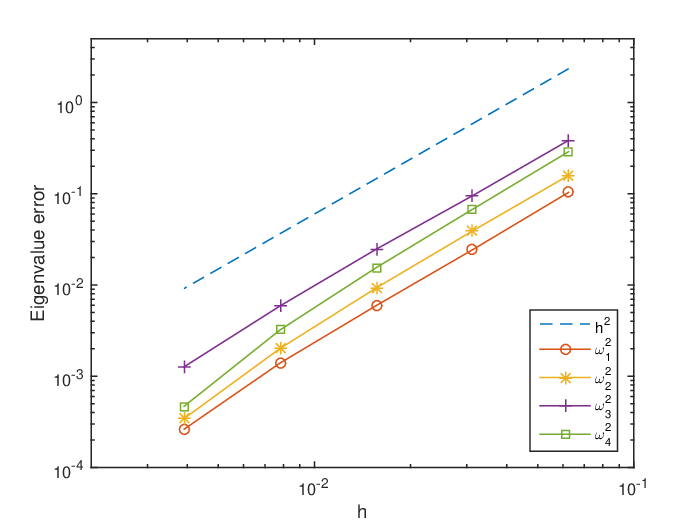


Example5 (Incompressible materials) To experiment the case of the incompressible elastic materials, we set and . We carry out similar numerical experiments with a straight-line interface to demonstrate the locking-free character of our method. The domain and interface are the same as Example 3. In Figure 11, we report the computed errors of first four eigenvalues by IFEM. According to Figure 11, it can be seen that the method has thoroughly locking-free feature for solving the elasticity interface problems.


References
- [1] Green D, Unruh WG. The failure of the Tacoma bridge: a physical model. American Journal of Physics 2006; 74 : 706–716.
- [2] Trefethen LN, Betcke T. Computed eigenmodes of planar regions. Recent advances in differential equations and mathematical physics, Contemporary Mathematics, 412, American Mathematical Society, Providence 2006; 297–314.
- [3] Armentano MG, Durán RG. Asymptotic lower bounds for eigenvalues by nonconforming finite element methods. Electronic Transactions on Numerical Analysis 2004; 17 : 93–101.
- [4] Carstensen C, Gedicke J. Guaranteed lower bounds for eigenvalues. Mathematics of Computation 2014; 83 : 2605–2629.
- [5] Walsh TF, Reese GM, Hetmaniuk UL. Explicit a posteriori error estimates for eigenvalue analysis of heterogeneous elastic structures. Computer Methods in Applied Mechanics and Engineering 2007; 196 : 3614–3623.
- [6] Oden JT, Prudhomme S, Westermann T, Bass J, Botkin ME. Error estimation of eigenfrequencies for elasticity and shell problems. Mathematical Models and Methods in Applied Sciences 2003; 13 : 323–344.
- [7] Hernández E. Finite element approximation of the elasticity spectral problem on curved domains. Journal of Computational and Applied Mathematics 2009; 225 : 452–458.
- [8] Meddahi S, Mora D, Rodríguez R. Finite element spectral analysis for the mixed formulation of the elasticity equations. SIAM Journal on Numerical Analysis 2013; 51 : 1041–1063.
- [9] Chang KS, Kwak DY. Discontinuous bubble scheme for elliptic problems with jumps in the solution. Computer Methods in Applied Mechanics and Engineering 2011; 200 : 494–508.
- [10] Chou SH, Kwak DY, Wee KT. Optimal convergence analysis of an immersed interface finite element method. Advances in Computational Mathematics 2010; 33 : 149–168.
- [11] Kwak DY, Wee KT, Chang KS. An analysis of a broken -nonconforming finite element method for interface problems. SIAM Journal on Numerical Analysis 2010; 48 : 2117–2134.
- [12] Li Z, Lin T, Lin Y, Rogers RC. An immersed finite element space and its approximation capability. Numerical Methods for Partial Differential Equations 2004; 20 : 338–367.
- [13] Li Z, Lin T, Wu X. New Cartesian grid methods for interface problems using the finite element formulation. Numerische Mathematik 2003; 96 : 61–98.
- [14] Kwak DY, Jin S. A stabilized immersed finite element method for the interface elasticity problems. arXiv:1408.4227.
- [15] Crouzeix M, Raviart PA. Conforming and nonconforming finite element methods for solving the stationary Stokes equations I. Revue Française Automatique Informatique Recherche Opérationnelle Série Rouge 1973; 7(R-3) : 33–75.
- [16] Lin T, Sheen D, Zhang X. A locking-free immersed finite element method for planar elasticity interface problems. Journal of Computational Physics 2013; 247 : 228–247.
- [17] Lin T, Zhang X. Linear and bilinear immersed finite elements for planar elasticity interface problems. Journal of Computational and Applied Mathematics 2012; 236 : 4681–4699.
- [18] Lee S, Kwak DY, Sim I. Immersed finite element method for eigenvalue problem. arXiv:1412.3163.
- [19] Brenner SC, Sung LY. Linear finite element methods for planar linear elasticity. Mathematics of Computation 1992; 59 : 321–338.
- [20] Hansbo P, Larson MG. Discontinuous Galerkin and the Crouzeix-Raviart element: Applications to elasticity. Mathematical Modelling and Numerical Analysis 2003; 37 : 63–72.
- [21] Babuška I, Osborn JE. Eigenvalue problems. Handbook of Numerical Analysis II. North-Holland: Amsterdam, 1991.
- [22] Descloux J, Nassif N, Rappaz J. On spectral approximation. I. The problem of convergence. RAIRO Analyse Numérique 1978; 12 : 97–112.
- [23] Descloux J, Nassif N, Rappaz J. On spectral approximation. II. Error estimates for the Galerkin method. RAIRO Analyse Numérique 1978; 12 : 113–119.
- [24] Osborn JE. Spectral approximation for compact operators. Mathematics of Computation 1975; 29 : 712–725.
- [25] Alonso A, Dello Russo A. Spectral approximation of variationally-posed eigenvalue problems by nonconforming methods. Journal of Computational and Applied Mathematics 2009; 223 : 177–197.
- [26] Antonietti PF, Buffa A, Perugia I. Discontinuous Galerkin approximation of the Laplace eigenproblem. Computer Methods in Applied Mechanics and Engineering 2006; 195 : 3483–3503.
- [27] Beattie C. Galerkin eigenvector approximations. Mathematics of Computation 2000; 69 : 1409–1434.
- [28] Buffa A, Perugia I. Discontinuous Galerkin approximation of the Maxwell eigenproblem. SIAM Journal on Numerical Analysis 2006; 44 : 2198–2226.
- [29] Braess D. Finite elements. Theory, fast solvers, and applications in solid mechanics. 2nd ed., Cambridge University Press: Cambridge, 2001.
- [30] Hansbo A, Hansbo P. A finite element method for the simulation of strong and weak discontinuities in solid mechanics. Computer Methods in Applied Mechanics and Engineering 2004; 193 : 3523–3540.
- [31] Leguillon D, Sánchez-Palencia E. Computation of singular solutions in elliptic problems and elasticity. John Wiley & Sons, Ltd., Chichester: Masson, Paris, 1987.
- [32] Kato T. Perturbation theory for linear operators. Classics in Mathematics, Springer-Verlag: Berlin, 1995.
- [33] Lehoucq RB, Sorensen DC, Yang C. ARPACK users’ guide: solution of large-scale eigenvalue problems with implicitly restarted Arnoldi methods. SIAM: Philadelphia, 1998.