Fidelity and Fisher information on quantum channels

Fidelity, as a measure of the distinguishability between quantum states[1, 2, 3], plays an important role in many areas of quantum information science, for example it is related to the precision limit in quantum metrology [4], serves as a measure of entanglement preservation through noisy quantum channels [5], and a measure of entanglement preservation in quantum memory [6]; it has also been used as a characterization method for quantum phase transitions [7], and a criterion for successful transmission in formulating quantum channel capacities [8].

Unlike the fidelity of quantum states which is defined directly on quantum states, most commonly used measures for the distinguishability of quantum channels are defined indirectly through the effects of the channels on the states. For example the diamond norm, which is defined as $\|K_{1}-K_{2}\|_{\diamond}=\max_{\rho_{SA}}\|K_{1}\otimes I_{A}(\rho_{SA})-K_{2}\otimes I_{A}(\rho_{SA})\|_{1}$[9, 10, 11]( here $\|X\|_{1}=Tr\sqrt{X^{\dagger}X}$, $\rho_{SA}$ denotes a state on system+ancilla, and $I_{A}$ denotes the identity operator on the ancillary system), is induced by the trace distance on quantum states $\|\rho_{1}-\rho_{2}\|_{1}$; another measure on quantum channels which is defined as $\arccos F_{\min}(K_{1},K_{2})=\arccos\min_{\rho_{SA}}F_{S}[K_{1}\otimes I_{A}(\rho_{SA}),K_{2}\otimes I_{A}(\rho_{SA})]$[12, 13], is induced by the fidelity on quantum states $F_{S}(\rho_{1},\rho_{2})=Tr\sqrt{\rho_{1}^{\frac{1}{2}}\rho_{2}\rho_{1}^{\frac{1}{2}}}$. These induced measures through quantum states lack a direct connection to the properties of quantum channels, which severely restrict the insights that can be gained from these measures. A direct measure on quantum channels is expected to provide more insights thus highly desired.

In this paper we provide a fidelity function defined directly on quantum channels, and show that this fidelity function on quantum channels, together with the classical fidelity on probability distribution and the fidelity on quantum states, form a hierarchy of fidelity functions in terms of optimization. This fidelity function on quantum channels also lead to various distance measures defined directly on quantum channels, in particular we show the Bures angle and the Bures distance can be extended to quantum channels. We then show the distance between quantum channels leads naturally to a new Fisher information on quantum channels which quantifies the ultimate precision limit in quantum metrology. We also show that this fidelity function provides a unified framework for perfect quantum channel discrimination and quantum metrology, in particular we show the minimum number of uses needed for perfect channel discrimination is exactly the counterpart of the precision limit in quantum metrology, and various useful lower bounds for the minimum number of uses needed for perfect channel discrimination can be obtained via this connection.

We start by defining the fidelity function on unitary channels then extend it to noisy channels.

For a $m\times m$ unitary matrix $U$, we denote $e^{-i\theta_{j}}$ as the eigenvalues of $U$, where $\theta_{j}\in(-\pi,\pi]$ for $1\leq j\leq m$ and we call $\theta_{j}$ the eigen-angles of $U$. We define(see also[14, 15, 16]) $\parallel U\parallel_{\max}=\max_{1\leq j\leq m}\mid\theta_{j}\mid,$ and $\parallel U\parallel_{g}$ as the minimum of $\parallel e^{i\gamma}U\parallel_{\max}$ over equivalent unitary operators with different global phases, i.e., $\parallel U\parallel_{g}=\min_{\gamma\in\mathbb{R}}\parallel e^{i\gamma}U\parallel_{\max}$. We then define

Quantitatively $C(U)$ is equal to the maximal angle that $U$ can rotate a state away from itself[17, 21, 16], i.e., $\cos[C(U)]=\min_{|\psi\rangle}|\langle\psi|U|\psi\rangle|.$ For mixed states it can be written as $\cos[C(U)]=\min_{\rho}F_{S}(\rho,U\rho U^{\dagger}).$

If $\theta_{\max}=\theta_{1}\geq\theta_{2}\geq\cdots\geq\theta_{m}=\theta_{\min}$ are arranged in decreasing order, then $C(U)=\frac{\theta_{\max}-\theta_{\min}}{2}$ when $\theta_{\max}-\theta_{\min}\leq\pi$[16]. We then define $\Theta_{QC}(U_{1},U_{2})=C(U_{1}^{\dagger}U_{2})$, here $U_{1}$ and $U_{2}$ are unitary operators on the same Hilbert space(we can expand the space if they are not the same). It is easy to see that

$\Theta_{QC}(U_{1},U_{2})$ thus corresponds to the maximal angle between the output states of $U_{1}$ and $U_{2}$(however we note that the definition of $\Theta_{QC}(U_{1},U_{2})$ is independent of the states). We then denote $F_{QC}(U_{1},U_{2})=\cos[\Theta_{QC}(U_{1},U_{2})]$ as the fidelity between $U_{1}$ and $U_{2}$. For unitary channels this is equivalent to the fidelity function proposed previously in [17].

We now generalize this to noisy quantum channels. A general quantum channel $K$, which maps from $m_{1}$- to $m_{2}$-dimensional Hilbert space, can be represented by Kraus operators, $K(\rho_{S})=\sum_{j=1}^{q}F_{j}\rho_{S}F^{\dagger}_{j}$ where $\sum_{j=1}^{q}F^{\dagger}_{j}F_{j}=I$. Equivalently it can also be written as $K(\rho_{S})=Tr_{E}(U_{ES}(|0_{E}\rangle\langle 0_{E}|\otimes\rho_{S})U^{\dagger}_{ES}),$ where $|0_{E}\rangle$ denotes some standard state of the environment, and $U_{ES}$ is a unitary operator acting on both system and environment, which we call as the unitary extension of $K$.

We define $\Theta_{QC}(K_{1},K_{2})=\min_{\{U_{ES1},U_{ES2}\}}\Theta_{QC}(U_{ES1},U_{ES2})$ and $F_{QC}(K_{1},K_{2})=\cos\Theta_{QC}(K_{1},K_{2}),$ where $U_{ESi}$ are unitary extensions of $K_{i}$, $i\in\{1,2\}$. In Appendix A, we show that the optimization can be taken by fixing one unitary extension and just optimizing over the other unitary extension, i.e.,

In terms of $F_{QC}(K_{1},K_{2})$ it can be written as

This can be seen as the counterpart of Uhlmann’s purification theorem on quantum states [22](however the proof does not use Uhlmann’s purification theorem [18]). In Appendix B, we show that $\Theta_{QC}(K_{1},K_{2})$ is a metric and can be computed directly from the Kraus operators of $K_{1}$ and $K_{2}$ as [18]

here $\lambda_{\min}(K_{W}+K^{\dagger}_{W})$ denotes the minimum eigenvalue of $K_{W}+K^{\dagger}_{W}$ with $K_{W}=\sum_{ij}w_{ij}F_{1i}^{\dagger}F_{2j}$, $F_{1i}$ and $F_{2j}$ denote the Kraus operators of $K_{1}$ and $K_{2}$ respectively, $w_{ij}$ denotes the $ij$-th entry of a $q\times q$ matrix $W$ with $\|W\|\leq 1$ where $\|\cdot\|$ is the operator norm which corresponds to the maximum singular value, here $W$ arises from the non-uniqueness of the Kraus representations. Thus

We emphasize that $F_{QC}$ is defined directly on quantum channels without referring to the states, such direct connection, in contrast to the induced measure, is crucial when applying the fidelity to channel discrimination and quantum metrology as we will show later. Furthermore the fidelity can be formulated as a semi-definite programming and computed efficiently as $\max_{\|W\|\leq 1}\frac{1}{2}\lambda_{\min}(K_{W}+K^{\dagger}_{W})=$

Analogous to the Bures distance on quantum states $B_{S}(\rho_{1},\rho_{2})=\sqrt{2-2F_{S}(\rho_{1},\rho_{2})}$, we can similarly define a Bures distance on quantum channels as $B_{QC}(K_{1},K_{2})=\sqrt{2-2F_{QC}(K_{1},K_{2})}$. In Appendix A, we prove an intriguing and useful connection between $B_{QC}(K_{1},K_{2})$ and the minimum distances between the Kraus operators of $K_{1}$ and $K_{2}$ as

where $\{\tilde{F}_{1i}\},\{\tilde{F}_{2i}\}$ are the sets of all equivalent Kraus representations of $K_{1}$ and $K_{2}$ respectively. This connection is particular useful in studying the scalings of the distance between quantum channels as we will show later.

In which sense we call $F_{QC}(K_{1},K_{2})$ a fidelity function? It turns out that $F_{QC}(K_{1},K_{2})=\min_{\rho_{SA}}F_{S}[K_{1}\otimes I_{A}(\rho_{SA}),K_{2}\otimes I_{A}(\rho_{SA})]$. To see this, it is proved in the supplemental material of Ref. [18] that

which coincides with Eq. (8). From this relationship it is also immediate clear that $F_{QC}(K_{1},K_{2})$ is stable, i.e., $F_{QC}(K_{1}\otimes I,K_{2}\otimes I)=F_{QC}(K_{1},K_{2})$. This result gives an operational meaning to $F_{QC}(K_{1},,K_{2})$. We emphasize that although we made connections between $F_{QC}(K_{1},K_{2})$ and the minimum fidelity of the output states, $F_{QC}(K_{1},K_{2})$ is defined directly on quantum channels and does not depend on the states. The definition and the operational meaning of $F_{QC}(K_{1},K_{2})$ play distinct roles in applications, the operational meaning provides a physical picture while the direct definition brings insights which enable or ease the proofs and computations, which will be demonstrated in the applications. This is in analogy to how fidelity of quantum states is connected to the classical fidelity $F_{S}(\rho_{1},\rho_{2})=\min_{\{E_{i}\}}F_{C}(p_{1},p_{2})$, here $F_{C}(p_{1},p_{2})=\sum_{i}\sqrt{p_{1i}}\sqrt{p_{2i}}$ denotes the classical fidelity with $p_{1i}=Tr(\rho_{1}E_{i})$ and $p_{2i}=Tr(\rho_{2}E_{i})$, $\{E_{i}\}$ denotes a set of Positive Operator Valued Measurements(POVM)[3], here similarly the fidelity between quantum states has the operational meaning as the minimum classical fidelity, however the fidelity between quantum states is defined directly on quantum states which is independent of the measurements and such direct definition has provided numerous insights which would be hindered with just the classical fidelity.

It is known that the trace distance and the fidelity between quantum states have the following relationships[19]

from which it is straightforward to get the relationships between the diamond norm and the fidelity of quantum channels. This can be obtained by substituting $\rho_{1}=K_{1}\otimes I_{A}(\rho_{SA})$ and $\rho_{2}=K_{2}\otimes I_{A}(\rho_{SA})$, then optimizing over $\rho_{SA}$

which gives

Since $F_{QC}(K_{1},K_{2})$ can be computed directly from the Kraus operators, this also provides a way to bound the diamond norm using the Kraus operators.

In [20] the Choi matrices of the quantum channels are used to compute the fidelity between the channels, which corresponds to the fidelity between the output states of two quantum channels when the input state is taken as the maximal entangled state. As the maximal entangled state is in general not the optimal input state, the fidelity thus defined does not have operational meaning as the minimum fidelity of the output states, thus can not be related to the ultimate precision limit in quantum metrology etc(instead related to the precision limit when the probe state is taken as the maximally entangled state).

Next we demonstrate the applications in quantum information science, in particular we show how the fidelity provides a unified platform for the ultimate precision in quantum metrology and the minimum number of uses needed for perfect channel discrimination.

The task of quantum metrology, or quantum parameter estimation in general, is to estimate a parameter $x$ encoded in some channel $K_{x}$, this can be achieved by preparing a quantum state $\rho_{SA}$ and let it go through the extended channel $K_{x}\otimes I_{A}$ with the output state $\rho_{x}=K_{x}\otimes I_{A}(\rho_{SA})$. By performing POVM, $\{E_{y}\}$, on $\rho_{x}$ one gets the measurement result $y$ with probability $p(y|x)=Tr(E_{y}\rho_{x})$. According to the Cramér-Rao bound[24, 25, 26, 27], the standard deviation for any unbiased estimator of $x$ is bounded below by $\delta\hat{x}\geq\frac{1}{\sqrt{nJ_{C}[p(y|x)]}},$ where $\delta\hat{x}$ is the standard deviation of the estimation of $x$, $J_{C}[p(y|x)]$ is the classical Fisher information and $n$ is the number of times that the procedure is repeated. The classical Fisher information can be further optimized over all POVMs, which gives

where the optimized value $J_{S}(\rho_{x}$) is usually called the quantum Fisher information[24, 25, 4, 28], here for distinguish we will call it the quantum state Fisher information.

We first recall established connections between the fidelity functions and the Fisher information. Given $\rho_{x}$ and its infinitesimal state $\rho_{x+dx}$, for a given POVM $\{E_{y}\}$, the classical fidelity between $p(y|x)=Tr(E_{y}\rho_{x})$ and $p(y|x+dx)=Tr(E_{y}\rho_{x+dx})$ is given by $F_{C}[p(y|x),p(y|x+dx)]=\sum_{y_{i}}\sqrt{p(y_{i}|x)}\sqrt{p(y_{i}|x+dx)}$ which defines an angle as $\cos\Theta_{C}[p(y|x),p(y|x+dx)]=F_{C}[p(y|x),p(y|x+dx)]$. The classical Fisher information is related to the classical fidelity as $\frac{1}{4}J_{C}[p(y|x)]dx^{2}=2-2F_{C}[p(y|x),p(y|x+dx)]$ up to the second order of $dx$[4], this can also be written as

If we optimize over $\{E_{y}\}$ the classical fidelity then leads to the fidelity between quantum states as [4]

and the classical Fisher information leads to the quantum state Fisher information $J_{S}(\rho_{x})=\max_{\{E_{y}\}}J_{C}[p(y|x)]$ and up to the second order of $dx$[4, 28]

If we denote $\cos\Theta_{S}(\rho_{x},\rho_{x+dx})=F_{S}(\rho_{x},\rho_{x+dx})$, then

The precision can be further improved by optimizing over the probe states, which leads to the ultimate local precision limit of estimating $x$ from $K_{x}$. Intuitively, this ultimate precision limit should be quantified by the distance between $K_{x}$ and its infinitesimal neighboring channel $K_{x+dx}$, in a way analogous to how Bures distance of quantum states quantifies the precision limit of estimating $x$ from the state $\rho_{x}$[4]. However although much progress has been made on calculating the ultimate precision limit[29, 30, 31, 32, 33, 34, 35, 36, 37], such a clear physical picture has still not been established after more than two decades since Braunstein and Caves’s seminal paper[4], this is mainly due to the lack of proper tools on quantum channels. Here we show that the fidelity between quantum channels can be used to establish such a physical picture, which also leads naturally to a new Fisher information on quantum channel.

Further optimizing over the probe states

this leads naturally to a quantum channel Fisher information $J_{QC}(K_{x})=\max_{\rho_{SA}}J_{S}(\rho_{x})$ which is similarly related to the distance on quantum channels as

The quantum channel Fisher information quantifies the ultimate precision limit upon the optimization over the measurements and probe states

This connects the precision limit directly to the distance between quantum channels which provides a clear physical picture for the ultimate precision limit. The scaling of the ultimate precision limit can now be seen as a manifestation of the scaling of the distances between quantum channels as we now show.

Two schemes on multiple uses of quantum channels are usually considered in quantum parameter estimation, the parallel scheme and the sequential scheme as shown in Fig.1. We will show that for both schemes, the scaling of the distances between two quantum channels are at most linear, which underlies the scaling for the Heisenberg limit.

For parallel scheme with $N$ uses of a channel $K$ as shown in Fig.3, the total dynamics can be described by $K^{\otimes N}\otimes I_{A}$. If we denote $U_{ES}$ as one unitary extension of $K$, then $U_{ES}^{\otimes N}$ is a unitary extension of $K^{\otimes N}$ as shown in Fig.3. Given two channels $K_{1}$ and $K_{2}$, we choose $U_{ES1}$ and $U_{ES2}$ as the unitary extension for $K_{1}$ and $K_{2}$ respectively which satisfies $\Theta_{QC}(K_{1},K_{2})=\Theta_{QC}(U_{ES1},U_{ES2})$. Now as $U_{ES1}^{\otimes N}$ and $U_{ES2}^{\otimes N}$ are unitary extensions of $K_{1}^{\otimes N}$ and $K_{2}^{\otimes N}$ respectively, we then have

For the sequential scheme, we consider the general case that controls can be inserted between sequential uses of the channels. Any measurements that are used in the control can be substituted by controlled unitaries with ancillary systems, the controls interspersed between the channels can thus be taken as unitaries, which is shown in Fig.5. Parallel scheme can be seen as a special case of the sequential scheme by choosing the controls as SWAP gates on the system and different ancillary systems[36]. We show that with $N$ uses of the channel, the distance is still bounded above by $N\Theta_{QC}(K_{1},K_{2})$.

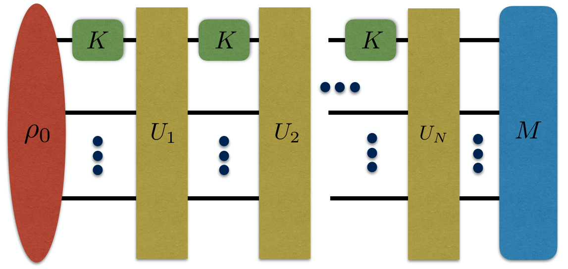
We present the proof for the case of $N=2$, same line of argument works for general $N$. For $N=2$, one unitary extension of $U_{2}K_{1}U_{1}K_{1}$ is $U_{2}U_{E_{2}S1}U_{1}U_{E_{1}S1}$, similarly $U_{2}U_{E_{2}S2}U_{1}U_{E_{1}S2}$ is a unitary extension of $U_{2}K_{2}U_{1}K_{2}$, here $U_{E_{j}Si}$ denote a unitary extension of $K_{i}$, $i=1,2$, with $E_{j}$ as the environment. We can choose $U_{E_{j}Si}$ such that $\Theta_{QC}(K_{1},K_{2})=\Theta_{QC}(U_{E_{j}S1},U_{E_{j}S2})$, here all operators are understood as defined on the whole space so the multiplication makes sense, for example the control $U_{1}$, which only acts on the system and ancillaries, is understood as $U_{1}\otimes I_{E}$, an operator on the whole space including the environment. We then have

i.e., with two uses of the channel, the distance is bounded above by $2\Theta_{QC}(K_{1},K_{2})$. With the same line of argument it is easy to show that with $N$ uses of the channel the distance is bounded above by $N\Theta_{QC}(K_{1},K_{2})$.

Substitute $K_{1}$ with $K_{x}$ and $K_{2}$ with $K_{x+dx}$, we have $\Theta_{QC}(NK_{x},NK_{x+dx})\leq N\Theta_{QC}(K_{x},K_{x+dx})$ for both schemes. From Eq.(21) the ultimate precision limit is then bounded by

the scaling $1/N$ is called the Heisenberg scaling, which, as we showed, is just a manifestation of the fact that the distance between quantum channels can grow at most linearly with the number of channels.

For $N$ uses of the channels under the parallel scheme we can also obtain a tighter bound as

here $K_{W}=\sum_{i=1}^{q}\sum_{j=1}^{q}w_{ij}F_{1i}^{\dagger}F_{2j}$ as previously defined, and the inequality holds for any $W$ with $\|W\|\leq 1$ (see Appendix C). In the asymptotical limit, $N(N-1)\|I-K_{W}\|^{2}$ is the dominating term, in that case we would like to choose a $W$ minimizing $\|I-K_{W}\|$ to get a tighter bound. This can be formulated as semi-definite programming with $\min_{\|W\|\leq 1}\|I-K_{W}\|=$

If we let $K_{1}=K_{x}$ and $K_{2}=K_{x+dx}$, then Eq.(25) provides bounds on the scalings in quantum parameter estimation, which is consistent with the studies in quantum metrology[29, 30, 32, 35, 36] but here with a more general context (see also Ref. [18]).

Next we show how the tools unify quantum parameter estimation and the perfect quantum channel discrimination[17, 38, 39, 40, 41, 42, 43].

Given two quantum channels $K_{1}$ and $K_{2}$, they can be perfectly discriminated with one use of the channels if and only if there exists a $\rho_{SA}$ such that $K_{1}\otimes I_{A}(\rho_{SA})$ and $K_{2}\otimes I_{A}(\rho_{SA})$ are orthogonal, i.e., $\min_{\rho_{SA}}F_{S}[K_{1}\otimes I_{A}(\rho_{SA}),K_{2}\otimes I_{A}(\rho_{SA})]=0$, which is the same as $\Theta_{QC}(K_{1},K_{2})=\frac{\pi}{2}$. When $K_{1}$ and $K_{2}$ can not be perfectly discriminated with one use of the channel, finite number of uses may able to achieve the task[42]. This is in contrast to the perfect discrimination of non-orthogonal states which always requires infinite number of copies. The minimum number of uses needed for perfect channel discrimination should satisfy $\Theta_{QC}(NK_{1},NK_{2})=\frac{\pi}{2}$. The perfect channel discrimination is thus determined by the distances between quantum channels, and the scalings of $\Theta_{QC}(NK_{1},NK_{2})$ obtained before can be used to determine the minimum $N$. For example, from $\Theta_{QC}(NK_{1},NK_{2})\leq N\Theta_{QC}(K_{1},K_{2})$ we can obtain a lower bound on $N$ as

where $\lceil x\rceil$ is the smallest integer not less than $x$. This bound is tighter than existing bounds for noisy channels[40] and for unitary channels it reduces to the formula which is known to be tight[17]. For noisy channels under the parallel scheme we can also substitute $\Theta_{QC}(K_{1}^{\otimes N},K_{2}^{\otimes N})=\frac{\pi}{2}$ into the inequality (25) to get a tighter bound.

The lower bound on minimum $N$ can also be obtained via a connection to quantum metrology. Given two channels $K_{1}$ and $K_{2}$, let $K_{x},x\in[a,b]$ as a path connecting $K_{1}$ and $K_{2}$. With $N$ uses of the channel under the parallel strategy we have $\sqrt{J_{QC}(K_{x}^{\otimes N})}=\lim_{dx\rightarrow 0}\frac{2\Theta_{QC}(K_{x}^{\otimes N},K_{x+dx}^{\otimes N})}{\mid dx\mid}$. From the triangular inequality

This connects the prefect channel discrimination to the ultimate precision limit. By choosing different paths various useful lower bounds on the minimum number of uses for perfect channel discrimination can be obtained.

For example, given $K_{0}(\rho)=e^{i\theta\sigma_{1}}\rho e^{-i\theta\sigma_{1}}$ and $K_{1}=\frac{1+\eta}{2}\rho+\frac{1-\eta}{2}\sigma_{3}\rho\sigma_{3}$, where $\sigma_{1},\sigma_{2}$ and $\sigma_{3}$ are Pauli matrices and assume $\theta=0.3,\eta=0.5$. For the parallel strategy the lower bound given by Eq.(27) is $N\geq\lceil\frac{\pi}{2\Theta_{QC}(K_{0},K_{1})}\rceil=3$. If we choose a simple path $K_{x}=(1-x)K_{0}+xK_{1}$, $x\in[0,1]$, which is a line segment connecting $K_{0}$ to $K_{1}$, then with the connection provided by Eq.(28) we obtain $N\geq 4$. Other paths may be explored to further improve the bound. By using the inequality (25) with the $W$ obtained from the semi-definite programming that minimizes $\|I-K_{W}\|$, we get $N\geq 5$. For any $N$ we can also choose the $W$ to minimize $N\|2I-K_{W}-K_{W}^{\dagger}\|+N(N-1)\|I-K_{W}\|^{2}$, it turns out the minimum $N$ such that $\min_{\|W\|\leq 1}N\|2I-K_{W}-K_{W}^{\dagger}\|+N(N-1)\|I-K_{W}\|^{2}\geq 2$ is $6$, thus $N\geq 6$. For comparison we also explicitly computed the actual distance $\Theta_{QC}(K_{0}^{\otimes N},K_{1}^{\otimes N})$ with the increasing of $N$, it turns out that the minimum $N$ such that $\Theta_{QC}(K_{0}^{\otimes N},K_{1}^{\otimes N})=\frac{\pi}{2}$ is actually $6$. All computations here are done with the CVX package in Matlab[44].

A fidelity function defined directly on quantum channels is provided, which leads to various distance measures defined directly on quantum channels, as well as a new Fisher information on quantum channel. This forms another hierarchy for fidelity functions and Fisher information as shown in the table:

References

- [1] C. A. Fuchs and C. M. Caves, Phys. Rev. Lett. 73, 3047 (1994), URL http://link.aps.org/doi/10.1103/PhysRevLett.73.3047.
- [2] R. Jozsa, Journal of Modern Optics 41, 2315 (1994), eprint http://dx.doi.org/10.1080/09500349414552171, URL http://dx.doi.org/10.1080/09500349414552171.
- [3] C. A. Fuchs, arXiv pp. quant–ph/9601020 (1996).
- [4] S. L. Braunstein and C. M. Caves, Phys. Rev. Lett. 72, 3439 (1994), URL http://link.aps.org/doi/10.1103/PhysRevLett.72.3439.
- [5] B. Schumacher, Phys. Rev. A 54, 2614 (1996), URL http://link.aps.org/doi/10.1103/PhysRevA.54.2614.
- [6] K. Surmacz, J. Nunn, F. C. Waldermann, Z. Wang, I. A. Walmsley, and D. Jaksch, Phys. Rev. A 74, 050302 (2006), URL http://link.aps.org/doi/10.1103/PhysRevA.74.050302.
- [7] S.-J. Gu, Int. J. Mod. Phys. B 24, 4371 (2010).
- [8] H. Barnum, E. Knill, and M. A. Nielsen, IEEE Trans. Info. Theor. 46, 1317 (2000), eprint quant-ph/9809010.
- [9] A. Kitaev, Russian Mathematical Surveys 52, 1191 (1997), URL http://www.turpion.org/php/paper.phtml?journal_id=rm&paper_id=2155.
- [10] A. Y. Kitaev, A. H. Shen, and M. N. Vyalyi, Classical and Quantum Computation (American Mathematical Society, Boston, MA, USA, 2002), ISBN 0821832298.
- [11] J. Watrous, arXiv p. 0901.4709 (2009).
- [12] A. Gilchrist, N. K. Langford, and M. A. Nielsen, Phys. Rev. A 71, 062310 (2005), URL http://link.aps.org/doi/10.1103/PhysRevA.71.062310.
- [13] V. P. Belavkin, G. M. D’Ariano, and M. Raginsky, J. Mathematical Physics 46, 062106 (2005).
- [14] H. F. Chau, Quant. Inf. Comput. 11, 0721 (2011).
- [15] C.-H. F. Fung and H. F. Chau, Phys. Rev. A 88, 012307 (2013), URL http://link.aps.org/doi/10.1103/PhysRevA.88.012307.
- [16] C.-H. F. Fung and H. F. Chau, Phys. Rev. A 90, 022333 (2014), URL http://link.aps.org/doi/10.1103/PhysRevA.90.022333.
- [17] A. Acin, Phys. Rev. Lett. 87, 177901 (2001), URL http://link.aps.org/doi/10.1103/PhysRevLett.87.177901.
- [18] H. Yuan and C.-H. F. Fung, to appear in npj Quantum Information (2017).
- [19] C. A. Fuchs and J. van de Graaf, IEEE Trans. Inf. Theory 45, 1216 (1999).
- [20] Maxim Raginsky, Physics Letters A, 290, 11-18 (2001).
- [21] G. M. D’Ariano, P. Lo Presti, and M. G. A. Paris, Phys. Rev. Lett. 87, 270404 (2001), URL http://link.aps.org/doi/10.1103/PhysRevLett.87.270404.
- [22] A. Uhlmann, Rep. Math. Phys. 9, 273-279 (1976).
- [23] H. Yuan and C.-H. F. Fung, arXiv p. 1506.01909 (2015).
- [24] C. W. Helstrom, Quantum Detection and Estimation Theory (Academic Press, 1976).
- [25] A. S. Holevo, Probabilistic and Statistical Aspect of Quantum Theory (North-Holland, 1982).
- [26] H. Cramer, Mathematical Methods of Statistics (Princeton University,, 1946).
- [27] C. R. B. Rao, Calcutta Math. Soc. 37, 81 (1945).
- [28] S. L. Braunstein, C. M. Caves, and G. J. Milburn, Annals of Physics 247, 135 (1996).
- [29] A. Fujiwara and H. Imai, Journal of Physics A: Mathematical and Theoretical 41, 255304 (2008).
- [30] B. M. Escher, R. L. de Matos Filho, and L. Davidovich, Nature Physics 7, 406 (2011).
- [31] M. Tsang, New J. Phys. 15, 073005 (2013).
- [32] R. Demkowicz-Dobrzanski, J. Kolodynski, and M. Guta, Nature Communications 3, 1063 (2012).
- [33] S. Knysh, V. N. Smelyanskiy, and G. A. Durkin, Phys. Rev. A 83, 021804 (2011), URL http://link.aps.org/doi/10.1103/PhysRevA.83.021804.
- [34] S. Knysh, E. Chen, and G. Durkin, arXiv p. 1402.0495 (2014), URL http://arxiv.org/abs/1402.0495.
- [35] J. Kolodynski and R. Demkowicz-Dobrzanski, New J. Phys. 15, 073043 (2013).
- [36] R. Demkowicz-Dobrzański and L. Maccone, Phys. Rev. Lett. 113, 250801 (2014), URL http://link.aps.org/doi/10.1103/PhysRevLett.113.250801.
- [37] S. Alipour, M. Mehboudi, and A. T. Rezakhani, Phys. Rev. Lett. 112, 120405 (2014), URL http://link.aps.org/doi/10.1103/PhysRevLett.112.120405.
- [38] R. Duan, Y. Feng, and M. Ying, Phys. Rev. Lett. 98, 100503 (2007), URL http://link.aps.org/doi/10.1103/PhysRevLett.98.100503.
- [39] R. Duan, Y. Feng, and M. Ying, Phys. Rev. Lett. 100, 020503 (2008), URL http://link.aps.org/doi/10.1103/PhysRevLett.100.020503.
- [40] C. Lu, J. Chen, and R. Duan, Quantum Info. Comput. 12, 138 (2012), ISSN 1533-7146, URL http://dl.acm.org/citation.cfm?id=2231036.2231045.
- [41] G. Chiribella, G. M. D’Ariano, and P. Perinotti, Phys. Rev. Lett. 101, 180501 (2008), URL http://link.aps.org/doi/10.1103/PhysRevLett.101.180501.
- [42] R. Duan, Y. Feng, and M. Ying, Phys. Rev. Lett. 103, 210501 (2009), URL http://link.aps.org/doi/10.1103/PhysRevLett.103.210501.
- [43] A. W. Harrow, A. Hassidim, D. W. Leung, and J. Watrous, Phys. Rev. A 81, 032339 (2010), URL http://link.aps.org/doi/10.1103/PhysRevA.81.032339.
- [44] M. Grant and S. Boyd (2011), URL http://cvxr.com/cvx/.
- [45] M.D. Choi, and C.K. Li, J. Operator Theory. 46, 435 (2001).
- [46] C.-H. F. Fung, H. F. Chau, C.K. Li, and N.S. Sze, Quantum Information and Computation 15, 0685-0693 (2015).
- [47] A. Childs, J. Preskill, and J. Renes. Quantum information and precision measurement. Journal of Modern Optics, 47(2–3):155–176, 2000.
- [48] H. Yuan, C.-H. F. Fung, Phys. Rev. Lett. 115, 110401 (2015).