Many-body effects in graphene beyond the Dirac model with Coulomb interaction
Abstract
This paper is devoted to development of perturbation theory for studying the properties of graphene sheet of finite size, at nonzero temperature and chemical potential. The perturbation theory is based on the tight-binding Hamiltonian and arbitrary interaction potential between electrons, which is considered as a perturbation. One-loop corrections to the electron propagator and to the interaction potential at nonzero temperature and chemical potential are calculated. One-loop formulas for the energy spectrum of electrons in graphene, for the renormalized Fermi velocity and also for the dielectric permittivity are derived.
Keywords:
graphene, electron properties, Coulomb interaction, Monte-Carlo simulationspacs
73.22.Pr, 05.10.Ln, 11.15.HaI Introduction
Graphene is a two dimensional crystal composed of carbon atoms which are packed in a honeycomb (hexagonal) lattice [1, 2]. It attracts considerable interest because of its unique electronic properties; most of them are related to existence of two conical points in the electron energy spectrum (Fermi points) and “massless Dirac fermion” character of charge carriers with energy and momentum close to the Fermi points [3, 4, 5, 6, 7]. It results in numerous quantum relativistic phenomena such as Klein tunneling, minimal conductivity through evanescent waves, relativistic collapse at a supercritical charge, etc., establishing an interesting and fruitful relation between fundamental physics and materials science [8, 9, 10, 11, 12, 13]. The effective “velocity of light” (Fermi velocity) for the Dirac fermions in graphene is relatively small, , and the interaction between the quasiparticles in graphene can be approximated by the instantaneous Coulomb potential with the effective coupling constant11 1 In this paper we work in units . This interaction is therefore quite strong, which results in a rich variety of phenomena [12]. Within the Dirac model, before the experimental discovery of graphene, it was shown that the long-range character of Coulomb interaction results in a renormalization of the Fermi velocity which is divergent at zero temperature and zero doping leading to a non-Fermi-liquid behaviour [14]; this prediction has been recently confirmed experimentally [15, 16].
At the same time, Dirac model gives us many-body renormalization of electronic properties only for small coupling constant and only with the logarithmic accuracy. The higher-order terms were considered in Refs. [17, 18] but still within the Dirac model. To calculate quantitatively correctly these properties one needs to work with the lattice model and with a realistic potential of electron-electron interaction taking into account its screening by the -electrons. The corresponding first-principle results [19] can be parametrized by the phenomenological potential. This modification of the interaction potential at small scales in comparison with the bare Coulomb potential was proved to affect some graphene properties significantly (for instance, the phase diagram of graphene [20]).
The authors of papers [20, 21, 22] carried out the Monte-Carlo study of graphene properties based on the tight-binding Hamiltonian without the expansion near the Fermi points. Within this approach one can introduce an arbitrary phenomenological potential . Using the tight-binding Hamiltonian on the hexagonal lattice, we are going to build the perturbation theory in . We believe that the theory built in this way is important and interesting for the following reasons.
The theory based on the tight-binding Hamiltonian has more common features with real graphene physics than the effective theory based on the expansion in the vicinity of Dirac points. For instance, the tight-binding Hamiltonian “remembers” graphene properties such as geometry of hexagonal lattice or the natural energy scale such as -bandwidth, which are absent in the effective Dirac theory. Moreover, one can include a phenomenological potential in this theory, which is closer to the real graphene physics than the bare Coulomb potential.
In addition, the theory based on the tight-binding Hamiltonian and the phenomenological interaction can be easily improved. For instance, one can study the effects appearing due to the inclusion of the next-to-the-nearest-neighbour hopping or nonzero chemical potential. Note that such study cannot be carried out within the Monte-Carlo simulation because of the well known sign problem. Finally, if the electron properties of other nanomaterials are formulated in terms of the tight-binding Hamiltonian and the phenomenological potential, it makes no difficulties to apply the results of this paper to study these materials.
Lattice simulation of graphene were proved to be a very efficient and quickly developing approach for studying the properties of graphene [20, 21, 22, 23, 24, 25]. An important feature of all these simulations is that they are conducted at the finite lattice, at the finite temperature and with the finite discretization errors. In order to check the lattice results and estimate the discretization uncertainty in the weak coupling region it is very useful to develop the perturbation theory which accounts all these effects.
Strictly speaking, the theory with the arbitrary phenomenological potential is not renormalizable since it contains four-fermion terms. However, lattice formulation provides the ultraviolet (spacing between carbon atoms) and the infrared (the finite size of the lattice) regulators. For this reason the theory on the hexagonal lattice is well defined.
Finally, one should mention that the interaction in graphene is strong, so the application of the perturbation theory is questionable. However, we believe that even at the one-loop level one can study some important physical effects. One can also expect that the perturbation theory built in this paper can well describe graphene many-body effects similarly to the RPA based on effective theory of graphene[18].
This paper is organized as follows. In the next section we built the perturbation theory which is based on the tight binding Hamiltonian and arbitrary interaction potential between electrons. In the section 3 we calculate one-loop corrections to the electron propagator. The section 4 is devoted to the calculation of one-loop corrections to the interaction potential. Finally, in the last section we discuss and summarize the results of this paper.
II Partition function and Feynman rules
II.1 Geometry
We consider a hexagonal lattice with the torus topology. The example of such lattice, which consists of hexagons, is shown in Fig.1.
The hexagonal lattice is the composition of two triangular sublattices and . The sites belonging to the sublattices and are shown as rectangles and circles respectively. The Cartesian coordinates of any lattice site can be parametrised by three numbers , where is the sublattice index and , , so
| (1) | |||
| (2) |
The torus topology implies the following identification of coordinates:
| (3) |
Every site of the sublattice is connected to three sites of the sublattice . The vectors in -coordinates, connect to its neighbours :
| (4) |
In -coordinates these vectors read:
| (5) |
II.2 Tight-binding Hamiltonian with interactions
The electronic properties of graphene can be described by the tight-binding Hamiltonian:
| (6) |
where the summation is kept over the neighbouring graphene lattice sites and , is the hopping parameter. Operators , create and annihilate electron with spin at the lattice site . Note that one can also include the next-to-nearest neighbours hopping to the Hamiltonian (6), but for simplicity we restrict our consideration to the nearest neighbours.
We choose the vacuum state that satisfies the following conditions:
| (7) |
so there is an electron with spin at every lattice site and no electrons with spin . As our main goal is to calculate the partition function , which contains summation over all states, the specific choice of will not affect any physical results.
It is convenient to rewrite the Hamiltonian in terms of creation and annihilation operators for ”particles” and ”holes”, which read:
| (8) |
The plus sign is taken for and the minus sign for , where and are the triangular sublattices labels. After operators redefinition the ground state satisfies . Thereby, we interpret the absence of a valence electron as a positively charged ”hole” and an additional electron as a negatively charged ”particle”. In terms of these operators the tight-binding Hamiltonian is:
| (9) |
The charge operator now reads:
| (10) |
It easy to check that , which means that this vacuum is electrically neutral.
In some applications [20, 21] the mass term is introduced:
| (11) |
here the plus sign is taken for sublattice A and the minus sign — for sablattice B . This term explicitly breaks the symmetry between two sublattices.
In order to study the action of the chemical potential on graphene properties we introduce the term
| (12) |
It is known that the interaction between electrons plays an important role. This part of the Hamiltonian has the form:
| (13) |
The Coulomb potential is often used to describe the interaction. However, it was shown in [19], that the real potential dramatically deviates from the Coulomb law at small distances, which affects physical properties [20].
The aim of this paper is to study the properties of the electronic system, described by the Hamiltonian:
| (14) |
where is an arbitrary phenomenological interaction, treated as the perturbation.
II.3 Electronic spectrum of graphene without interaction
If the interaction is neglected22 2 In this subsection we consider graphene with zero chemical potential, one can easily find Hamiltonian spectrum and its eigenfunctions, which can be written as:
| (15) |
where is an additional label representing particles () and antiparticles (). The first vector component corresponds to the sublattice, similarly the second one corresponds to the sublattice. The Brillouin zone momentums are:
| (16) |
Indices , give the full set of the eigenfunctions for the torus topology of the graphene sheet.
The energy spectrum of the Hamiltonian is then:
| (17) |
The wave function components are
| (18) |
There exist two special momenta , such that and , called the Dirac points. There are two different Dirac positioned at: and .
For the massless fermions (), in the vicinity of the Dirac points the energy spectrum of the fermion quasiparticles is:
| (19) |
The linear spectrum of fermion excitations plays the central role in the effective theory of graphene.
II.4 Partition function
Let us consider a graphene sheet at the temperature . To write down the partition function for this graphene sample, one should handle the 4-fermion interaction operator which is contained in the Hamiltonian (14). So, before going to the partition function the interaction term of the Hamiltonian should be decomposed using the Hubbard-Stratonovich transformation:
| (20) |
In the last expression we introduced the Hubbard field , which carries the interaction. Note also that we have omitted the determinant of the which is not important for our calculations.
Now it causes no difficulties to write down the partition function in terms of the path integral. To this end, we divide the Euclidean time into parts with the size . We introduce the electron fields , the hole fields and the Hubbard field (which is called “photon” below) at each site of the lattice . The boundary conditions in Euclidean time direction are periodic for “photon” and antiperiodic for the fermion fields , . The boundary conditions for the spatial directions are periodic for all the fields.
Finally, the partition function for the model can be written as [20, 21]:
| (21) |
where the matrix reads (here and are sublattice indices):
| (22) | |||
| (23) |
To get the expression for the fermion operator one should take the formula for the and carry out the substitution , . Note that in the formula (23) the summation is taken over all the coordinates and over the sublattice indices, so the interaction potential is assumed to be a matrix
| (24) |
In the limit of expression (21) corresponds to the partition function of graphene sheet at the temperature . In some applications, for instance in the Monte-Carlo simulation of graphene [20, 21], one uses small but finite step . Some of the formulas below are written for the finite to have the possibility to estimate the discretization uncertainty.
II.5 Propagators
Using the expression for the partition function (21), one can write down free propagators for the corresponding fields (see Fig. 2).
- 1.
The electron propagator
(25) where was introduced in (17).
Note that the matrix is the matrix in the ”sublattice space”,
its elements correspond to the propagation between one sublattice ( and ) and different sublattices ( and ).
Figure 4: The interaction vertex of electron with two “photon” fields - 2.
The hole propagator can be obtained from the electron propagator with the substitution .
- 3.
The propagator of the “photon” field
The potential is instantaneous and acts in one Euclidean time slice.
Using the expressions for the partition function, for the electron and hole propagators one can show that in the limit the charge of graphene sheet is
| (26) |
as it should be.
II.6 Vertices
The partition function (21) takes into account the interactions between electrons/holes and “photons”. The interaction vertices of “photons” and electrons can be derived with an arbitrary accuracy through the expansion of the expression for the fermion operator:
| (27) |
in powers of . The simplest interaction vertex is shown in Fig. 3. Using the formula (27), one can show that
at the leading order approximation in –expansion this vertex can be written as follows
| (28) |
where are the sublattice indices.
The next vertex, which is required for the subsequent analysis and describes the interaction between two electrons and two “photons”, is shown in Fig. 4.
At the leading order approximation it can be written as:
| (29) |
There are also additional vertices, coupling electrons to “photons” (because the field stands in the exponent). However, they are suppressed by the additional factors and give no contribution to the final answer in the limit . Note also that in this section we presented only vertices with electrons. The vertices with holes can be found similarly.
III One-loop corrections to the electron propagator
First we are going to consider one-loop corrections at zero chemical potential and nonzero temperature. One-loop corrections to the electron propagator can be expressed in terms of the self-energy function :
| (30) |
At the leading order approximation there are two diagrams shown in Fig. 6, 6 that contribute to :

The inverse of the free electron propagator can be written in the following form (see formula (25)):
| (31) |
The final expression for is
| (32) |
From the formula (32) one can see that one-loop corrections are reduced to the renormalization of the mass and the function . The renormalized mass now depends on the point in the Brillouin zone and has the form
| (33) |
The expression for the renormalized function is
| (34) |
Thus one-loop corrections conserve the form of the propagator (25) and substitute the free mass and the function with the renormalized expressions (33), (34). From this one can conclude that the energy spectrum of the quasiparticles at the one-loop approximation is . In order to estimate the size of one-loop corrections in Fig. 7 we plot the energy spectrum profile of electron with Coulomb, screened Coulomb [19] interactions and without interactions. The calculation was carried out at at infinitely large lattice.
The formulas (33) and (34) can be used to reproduce well-known results of the effective theory of graphene and generalize them to the case of nonzero temperature. To this end, we consider large lattice with the Coulomb interactions between electrons near the Fermi point. Then the formulas (33) and (34) can be written as
| (35) |
where is the ultraviolet cut-off, is the Euler’s constant. These formulas are in agreement with the predictions of effective theory of graphene at the leading logarithmic accuracy [14, 26].


During the derivation of the formulas (35) we carried out the integration over the two-dimensional sphere of radius . It was also assumed that , is much larger than all other energy scales involved. Note that the theory is regularized by the temperature in the infrared region. Note also that the ratio of the ultraviolet and the infrared cut-offs under the logarithm is multiplied by the that considerably reduces the total renormalization of the Fermi velocity.
In order to study the finite density effects we consider one-loop corrections at zero temperature and nonzero chemical potential. In addition to the diagrams shown in Figures 6, 6 there is a contribution of the interaction of the electron propagator with vacuum represented by the diagram shown in Fig. 9. As before, one-loop corrections at nonzero lead to the renormalization of the parameters of free propagator preserving its structure. In particular, the mass and the function at one-loop approximation can be written as follows
| (36) |
In the limit of large lattice , Coulomb interaction and the linear electron spectrum near the Fermi point, the formulas (36) can be written as
| (37) |
Similarly to the case of nonzero temperature chemical potential plays the role of the infrared cut-off. It should be noted now that there are four scales that can play the role of the infrared cut-off: the fermion mass , the chemical potential, the temperature and the inverse lattice size. We believe that in the infrared limit the theory is regularized by the largest of these scales. Note that the formulas (35), (36) take these effects into account exactly.
Note also that the formulas (35) can be written in the form (37) if instead of one uses new ultraviolet cut off and substitute the chemical potential by the temperature.
For this reason at temperature equal to chemical potential the renormalization due to temperature
effects is a little bit larger than the renormalization due to nonzero chemical potential.
In this consideration we did not take the Debye screening of the interaction potential at large distances
and the screening of the Coulomb potential at small distances into account, that will be done in the last section.
IV One-loop corrections to “photon” propagator and dielectric permittivity of graphene
In this section we calculate one-loop correction to the instantaneous “photon” propagator: .
One-loop corrections to the propagator in the momentum space can be expressed in terms of the polarisation operator as
| (38) |
where are renormalized and tree level Fourier transforms of the potential, which are the matrices in the sublattice space. In the limit of and one-loop approximation the only diagram shown in Fig. 9 contributes.
The expression for the polarization operator at one-loop approximation can be written in the following form:
| (39) |
Using formulas (38), (39) one can show that at large distances and at small temperature the expression for the interaction potentials for all the sublattice indices take the form
| (40) |
where
| (41) | |||
Now one may see that at zero temperature the interaction potential is the Coulomb potential screened by the dielectric permittivity , which is in agreement with the RPA result [13]. At nonzero temperature there is a two-dimensional Debye screening of the Coulomb potential with the Debye mass , which agrees with the results of the paper [27].
Similarly one can study the question how the nonzero density acts on the dielectric permittivity of graphene. To get the expression for the polarization operator in this case one can use the formulas (39) and carry out the following substitution . It is not difficult to find out that at large distance the expression for the interaction potential has the form (40) with given by the equation (41) and the Debye mass
| (42) |
The last expression agrees with the RPA result [13].
At the end of this section we plot the dielectric permittivity of graphene obtained from formulas (38), (39) as a function of distance in units of the lattice spacing (Fig. 11). The calculation was carried out for suspended graphene with the interaction potential from paper [20] and for different external conditions: , eV ( cm-2) and eV, . In order to compare our results with RPA we plot the dielectric permittivity given by formula (41). For small distance we compared our results with the results of Monte-Carlo simulation [28]. It is seen that the Monte-Carlo results are in a good agreement with one-loop results.
V Discussion and conclusion
This paper is devoted to the perturbation theory which can be used for studying the properties of graphene at finite temperature and nonzero chemical potential. This perturbation theory is based on the tight-binding Hamiltonian on hexagonal lattice and arbitrary interaction potential between electrons, which is considered as a perturbation. We built the partition function for this theory, derived Feynman rules and expressions for free propagators.
As an example of the application we calculated one-loop corrections to the electron propagator. It was shown that one-loop corrections lead to the renormalization of the bare mass and the function conserving the structure of the propagator. Using this result we calculated one-loop energy spectrum of electrons, renormalized fermion mass and Fermi velocity.
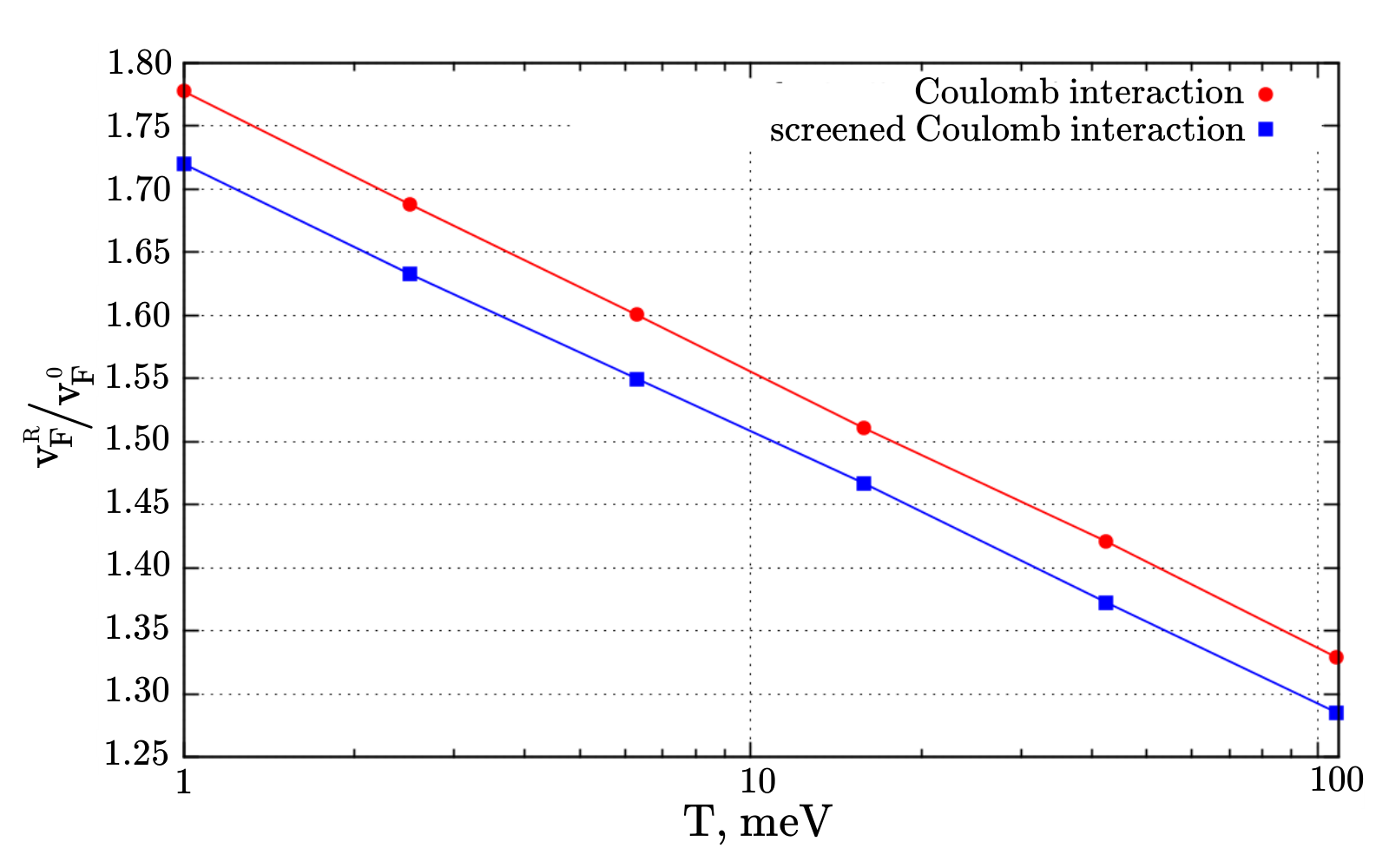
In order to estimate the value of the renormalization, in Fig. 11 we plotted the renormalization factor for the Fermi velocity as a function of the temperature for graphene on hBN for the Coulomb and screened at small distances Coulomb interactions [19]. During the calculation we took the screening of the potentials by the dielectric permittivity (38) into account. The results can be well described by the formula
| (43) |
where for the Coulomb interaction and for the screened Coulomb interaction . The effective ultraviolet cut-off is sensitive to the values of the potential at small distances, contrary to the coefficient . Note also that that the coefficient is well described by the expression .

In addition we considered one-loop corrections to the electron propagator at zero temperature and nonzero chemical potential. It was shown that similarly to the nonzero temperature case one-loop corrections conserve the structure of the propagator leading to the renormalization of already existing parameters. In particular, we obtained the formulas for the renormalization of the Fermi velocity and the fermion mass in this case.
In paper [16] the renormalization of the Fermi velocity was studied through the measurement of quantum capacitance at nonzero chemical potential. In this study the graphene layer was placed inside hBN, which reduced the strength of the interaction between electrons. This allows us to expect that perturbation theory works well in this case and we can compare our results with the the result of [16]. The results of the measurements of the Fermi velocity can be well fitted by the formula
| (44) |
where , and . Note that the original formula for the Fermi velocity from [16] depends on the density . In (44) we turn the dependence on to the dependence on chemical potential.
In the calculation we used the formulas (36) with the interaction potential screened by the dielectric permittivity (38). The interaction potential at small distances was taken from the paper [19] and divided by . At large distances we took the Coulomb potential screened by . The results of the calculations can be well fitted by formula (44) with the parameters: . This values are in reasonable agreement with paper [16]. In addition we carried out the calculation of the parameters for the Coulomb potential screened by . Our result is . Again we see that the value of the constant is sensitive to the values of the potential at small distances.
It is also interesting to compare the renormalization of the Fermi velocity due to nonzero and nonzero temperature. To this end we calculated nonzero temperature renormalization of the graphene layer placed inside the hBN for the Coulomb and screened at small distances Coulomb interactions. The results can be described by formula (43) with the parameters: for the Coulomb interaction and for the screened Coulomb interaction .
The other example of application of the perturbation theory is the calculation of one-loop corrections to the interaction potential done in the previous section. We derived the one-loop expression for the dielectric permittivity at nonzero temperature, nonzero chemical potential and the arbitrary interaction potential.
It is well known that the electrons in graphene form a strongly interacting system. So it is reasonable to consider the question how our results are affected by the higher order corrections. The authors of paper [18] considered the next-to-leading order (NLO) corrections to the Fermi velocity within effective theory of graphene. The main result of this paper in the statement that if one expands the Fermi velocity renormalization in the one-loop RPA potential instead of the usual Coulomb potential, the NLO corrections to the leading order(LO) result (37) turn out to be small. This allows us to expect a good accuracy of the formulas (33), (34), (36) with one-loop potential given by the formulas (38), (39) even for suspended graphene.
The authors of the paper [17] considered the NLO corrections to the polarization operator within the effective theory of graphene. The NLO value of the dielectric permittivity for suspended graphene is approximately by 30 % smaller than the LO result, which is not very large. Moreover, the Monte-Carlo results [28] tell us that the higher order corrections to the LO result can be even smaller than 30 %. For this reason one can expect that the accuracy of formulas (38), (39) is rather good.
Acknowledgements
We would like to thank M. Ulybyshev and A. Nikolaev for interesting discussions. MIK acknowledges financial support from NWO via Spinoza Prize. The work of VVB and NYB was supported by the Far Eastern Federal University, by RFBR grants 14-02-01261-a, 15-02-07596, 15-32-21117 and the Dynasty Foundation.
References
- [1] K. S. Novoselov, A. K. Geim, S. V. Morozov, D. Jiang, Y. Zhang, S. V. Dubonos, I. V. Grigorieva, and A. A. Firsov, Science 306, 666 (2004).
- [2] A. K. Geim and K. S. Novoselov, Nature Materials 6, 183 (2007).
- [3] P. R. Wallace, Phys. Rev. 71, 622 (1947).
- [4] J. W. McClure, Phys. Rev. 104, 666 (1956).
- [5] G. W. Semenoff, Phys. Rev. Lett. 53, 2449 (1984).
- [6] K. S. Novoselov, A. K. Geim, S. V. Morozov, D. Jiang, M. I. Katsnelson, I. V. Grigorieva, S. V. Dubonos, and A. A. Firsov, Nature 438, 197 (2005).
- [7] Y. Zhang, Y.-W. Tan, H. L. Stormer, and P. Kim, Nature 438, 201 (2005).
- [8] M. I. Katsnelson and K. S. Novoselov, Solid State Commun. 143, 3 (2007).
- [9] C. W. J. Beenakker, Rev. Mod. Phys. 80, 1337 (2008).
- [10] A. H. Castro Neto, F. Guinea, N. M. R. Peres, K. S. Novoselov, and A. K. Geim, Rev. Mod. Phys. 81, 109 (2009).
- [11] M. A. H. Vozmediano, M. I. Katsnelson, and F. Guinea, Phys. Rep. 496, 109 (2010).
- [12] V. N. Kotov, B. Uchoa, V. M. Pereira, F. Guinea, and A. H. Castro Neto, Rev. Mod. Phys. 84, 1067 (2012).
- [13] M. I. Katsnelson, Graphene: Carbon in Two Dimensions (Cambridge University Press, 2012).
- [14] J. Gonzalez, F. Guinea and M. A. H. Vozmediano, Nucl. Phys. B 424, 595 (1994).
- [15] D. C. Elias, R. V. Gorbachev, A. S. Mayorov, S. V. Morozov, A. A. Zhukov, P. Blake, L. A. Ponomarenko, I. V. Grigorieva, K. S. Novoselov, F. Guinea, and A. K. Geim, Nature Phys. 7, 701 (2011).
- [16] G. L. Yu, R. Jalil, B. Belle, A. S. Mayorov, P. Blake, F. Schedin, S. V. Morozov, L. A. Ponomarenko, F. Chiappini, S. Wiedmann, U. Zeitler, M. I. Katsnelson, A. K. Geim, K. S. Novoselov, and D. C. Elias, Proc. Nat. Acad. Sci. 110, 3282 (2013).
- [17] I. Sodemann and M. M. Fogler, Phys. Rev. B 86, 115408 (2012).
- [18] J. Hofmann, E. Barnes, and S. Das Sarma, Phys. Rev. Lett. 113, 105502 (2014).
- [19] T. O. Wehling, E. Sasioglu, C. Friedrich, A. I. Lichtenstein, M. I. Katsnelson, and S. Blugel, Phys. Rev. Lett. 106, 236805 (2011).
- [20] M. V. Ulybyshev, P. V. Buividovich, англи and M. I. Polikarpov, Phys. Rev. Lett. 111, 056801 (2013).
- [21] P. V. Buividovich and M. I. Polikarpov, Phys. Rev. B 86, 245117 (2012).
- [22] D. Smith and L. von Smekal, Phys. Rev. B 89, no. 19, 195429 (2014).
- [23] J. E. Drut and T. A. Lähde, Phys. Rev. Lett. 102, 026802 (2009); Phys. Rev. B 79, 165425 (2009); Phys. Rev. B 79, 241405 (2009);
- [24] W. Armour, S. Hands, and C. Strouthos, Phys. Rev. B 81, 125105 (2010); Phys. Rev. B 84, 075123 (2011).
- [25] P. V. Buividovich, E. V. Luschevskaya, O. V. Pavlovsky, M. I. Polikarpov and M. V. Ulybyshev, Phys. Rev. B 86, 045107 (2012).
- [26] V.N. Kotov, V.M. Pereira, and B. Uchoa, Phys. Rev. B 78, 075433 (2008).
- [27] V. V. Braguta, S. N. Valgushev, A. A. Nikolaev, M. I. Polikarpov and M. V. Ulybyshev, Phys. Rev. B 89, no. 19, 195401 (2014).
- [28] N. Yu. Astrakhantsev, V. V. Braguta, M. I. Katsnelson, A. A. Nikolaev, M. V. Ulybyshev, O. E. Soloveva, to be published.