Magnetic monopole - domain wall collisions

Let us consider a magnetic monopole whose winding lies in the 4-5 block of $\Phi$. This is possible [8] if we take the VEV along one of the radial directions far away from the monopole to be

The monopole ansatz for the scalar field can be written as [3]

while the non-zero gauge fields can be written as

and $P(r),M(r),N(r),$ and $K(r)$ are profile functions that depend only on the spherical radial coordinate $r=\sqrt{x^{2}+y^{2}+z^{2}}$ and satisfy the boundary conditions:

The profile functions for the monopole alone were evaluated numerically and are shown in Fig. 1.

The non-Abelian magnetic field can be defined as [9]

with the associated energy density given by ${\rm Tr}(B_{k}B^{k})$. Far away from the centre, the monopole field becomes $B^{k}\rightarrow Qx^{k}/(gr^{3})$, with $Q=\tau^{j}{x}^{j}/r$.

The monopole charge $Q$ includes a component along the generator of the unbroken $\mathrm{U}(1)$ symmetry ($\Phi_{\infty}$ of Eq. (8)), as well as $\mathrm{SU}(2)$ and $\mathrm{SU}(3)$ magnetic charges. The $\mathrm{U}(1)$ part of the magnetic field, which is a defining feature of a topological $\mathrm{SU}(5)$ monopole, is given by

where ${\hat{\phi}}^{a}\equiv\phi^{a}/\sqrt{\phi^{b}\phi^{b}}$. As discussed in [10], other definitions of the Abelian magnetic field are possible, and these differ from our definition but only within the core of the monopole. Since we only use our definition to plot the long range Abelian magnetic field (see Fig. 3) the definition in Eq. (12) is sufficient.

Without loss of generality [4], the domain wall solution can be taken to be diagonal at all $z$ and written in terms of the diagonal generators of $\mathrm{SU}(5)$ as

In each of the two disconnected parts of the vacuum manifold ${\cal M}$ there are a total of 10 different diagonal VEVs corresponding to all possible permutations of 2’s and 3’s in Eq. (6). Topology dictates that there must be a domain wall separating any pair of VEVs from the two disconnected parts of ${\cal M}$. However, not every such pair of VEVs corresponds to a stable domain wall solution. For instance, as shown in [3], the wall across which $\Phi_{0}$ goes to $-\Phi_{0}$ is unstable and will decay into a lower energy stable wall. The stable domain walls are obtained when both 3’s in Eq. (6) change into 2’s across the wall.

Let us choose the boundary condition at $z=-\infty$ to be

For this choice of $\Phi_{-}$, there are three different choices of $\Phi(z=+\infty)$, proportional to

that lead to stable domain walls. For the purpose of understanding the monopole-wall interactions, it is sufficient to consider only two of the above, corresponding to the two distinct entries in the 4-5 block of $\Phi$. We take the first to be the same as in [3], subsequently referred to as Case 1:

The value of the field in the core of this wall is proportional to $\text{diag}(1,-1,0,1,-1)$. The other case, subsequently referred to as Case 2, has

with the field in the wall being proportional to $\text{diag}(1,-1,1,0,-1)$. A novel feature of these walls is that the unbroken symmetry groups on either side of the wall are isomorphic to each other but they are realized along different directions of the initial $\mathrm{SU}(5)$ symmetry group. Hence the wall is the location of a clash of symmetries [12].

Note that the symmetry within the wall is [$\mathrm{SU}(2)\times\mathrm{U}(1)$]². The $\mathrm{SU}(2)$’s correspond to rotations in the 1-3 and 2-5 blocks and the $\mathrm{U}(1)$’s to rotations along $\sigma_{3}$ in the 1-2 and 3-5 blocks. Therefore the symmetry group within the wall is 8-dimensional, and is smaller than the 12-dimensional symmetry outside the wall¹¹ 1 For simplest domain walls, such as kinks in $\lambda\Phi^{4}$, the full symmetry of the Lagrangian is restored inside the core. However, the symmetry inside stable domain walls in $\mathrm{SU}(N)\times\mathrm{Z}_{2}$ is always lower than that of the vacuum [4].. Also note that the symmetry in the 4-5 block is different for the $\Phi^{(1)}_{+}$ and $\Phi^{(2)}_{+}$ vacua. This is going to be of direct relevance for the fate of the monopoles.

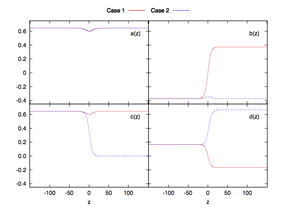
The profile functions $a(z)$, $b(z)$, $c(z)$ and $d(z)$ for both cases are shown in Fig. 2. In each case, they are linear combinations of two functions $F_{+}(z)$ and $F_{-}(z)$ defined by the alternative way of writing the domain wall solution [3]

where $F_{+}(\pm\infty)=1$, $F_{-}(\pm\infty)=\pm 1$. For a general choice of parameters, functions $F_{\pm}(z)$ must be found numerically. For $h/\lambda=-3/20$, they are known in closed form [3]: $F_{+}(z)=1$, $F_{-}(z)=\tanh(mz/\sqrt{2})$. Correspondingly, for this value of $h/\lambda$, the four functions $a(z)$, $b(z)$, $c(z)$, and $d(z)$ are either constant or describe a transition from one constant value to another. For $h/\lambda\neq-3/20$ the “constant” functions develop a small bump around $z=0$ as can be seen in Fig. 2.

As our initial configuration, we take the monopole to be on the $z=-\infty$ side, far away from the wall. In this case, the ansatz for the initial combined field configuration of the wall and the monopole can be written as [3]

where $z^{\prime}=\gamma(z-z_{0})$, $\gamma=1/\sqrt{1-v^{2}}$ is the boost factor, $v$ is the wall velocity and $z_{0}$ is the initial position of the wall. The monopole is at $x=0=y=z$. It is easy to check that, far away from the monopole, the profile functions take on the values in Eq. (11) and $\Phi_{M+DW}\rightarrow\Phi_{DW}$. Close to the monopole, $z^{\prime}\rightarrow-\infty$, since the monopole is initially very far from the wall, and $\Phi_{M+DW}\rightarrow\Phi_{M}$ as desired. We work in the temporal gauge, $X_{0}^{a}=0$, and with the initial ansatz for the gauge fields given by Eq. (10) for both cases.

It is instructive to examine the difference in the nature of the magnetic field in Cases 1 and 2. As mentioned in Sec. II.1, the charge of our monopole along the $z$-direction, $Q=(1/2)\text{diag}(0,0,0,1,-1)$, is a combination of the $\mathrm{U}(1)$, the $\mathrm{SU}(2)$, and the $\mathrm{SU}(3)$ magnetic charges. Since the VEV of $\Phi$ in our model is along the generator of (hypercharge) $\mathrm{U}(1)$, the magnetic field, as defined in Eq. (12), corresponds solely to the $\mathrm{U}(1)$ component of the charge. In Case 1, ${\rm Tr}(Q\Phi)$ is the same on both sides of the wall and the $\mathrm{U}(1)$ magnetic field is unaffected by the presence of the DW. In Case 2, however, ${\rm Tr}(Q\Phi^{(2)}_{+})=0$ and there is no magnetic field corresponding to the unbroken $\mathrm{U}(1)$ on the $z=+\infty$ side of the wall. Instead, the gauge field on that side is associated with an $\mathrm{SU}(2)$ subgroup of the unbroken $\mathrm{SU}(3)$. We note that, while the magnetic energy density associated with the gauge field is unaffected by the presence of the wall, it is specifically the $\mathrm{U}(1)$ magnetic field that is a defining feature of a topologically stable monopole.

The magnetic field, as defined in Eq. (12), is plotted for both cases in Fig. 3, where the vectors have components $r^{2}B_{Y}^{z}$ and $r^{2}B_{Y}^{x}$. This plot shows that, in Case 1, there is a $\mathrm{U}(1)$ magnetic field on both sides of the wall falling off as $r^{2}$ as expected, while in Case 2 the $\mathrm{U}(1)$ magnetic field is zero on the $z=+\infty$ side of the wall.

It is not difficult to predict that the monopole in Case 1 will pass through the wall. The monopole winding is due to the fields in the $\mathrm{SU}(2)$ subgroup corresponding to generators $\tau_{a}$, $a=1,..,3$. In Eq. (19), these fields are multiplied by the function $c(z)$ which has the same value at $z=\pm\infty$ and, as known from [3], is approximately constant across the domain wall. Only $b(z)$ and $d(z)$ change signs across the wall, but these are irrelevant for the winding of the monopole. Thus, the presence of the wall is of no qualitative consequence to the winding of the monopole or its profile functions. The only effect is the small change in $c(z)$ around $z=0$ (note that, as mentioned earlier, $c(z)$ is strictly a constant when $h/\lambda=-3/20$).

We numerically collide the monopole and the wall by giving the wall an initial velocity of $0.8$ (in speed of light units) and choosing parameters $\eta=1$, $h=-\lambda/5$, and $\lambda=0.5$ for $V(\Phi)$.

Fig. 4 shows the potential and magnetic energy densities as the wall hits the monopole in Case 1. In addition, we plot the scalar field configuration in Fig. 5, where each point is a vector with components $\phi^{3}$ and $\phi^{1}$. These figures show that the magnetic energy density and the scalar field configuration remain unchanged after the collision, and that the potential energy densities corresponding to the monopole and the domain wall remain localized. This does not imply a complete absence of interaction between the wall and the monopole – some interaction is expected due the non-linearity of the scalar field potential.

To see if the monopole gains momentum due to the interaction, we have evaluated the centre of energy (COE) defined as

where $V$ is the volume of a finite cylindrical region centred at the origin and extending $1/8$th of the lattice size in the $x$- and $z$-directions, while $\rho$ is the energy density. For $h/\lambda=0$, we give the wall a velocity of $v=0.9$ towards the monopole and compare the initial $z_{\rm CEO}$ to the one after the wall passes away. We see a very slow drift of the COE in the direction of the wall velocity. We performed the same procedure using different model parameters and wall velocities and the outcome was qualitatively the same. In all cases, while the direction of the drift is clear, the magnitude is extremely small and too close to the numerical uncertainties to allow a definitive quantitative analysis.

As in Case 1, it is possible to guess the outcome of the monopole-wall collision without doing numerical simulations. For this, we note that $\Phi^{(2)}_{+}$ has an $\mathrm{SU}(2)$ symmetry in the 4-5 block, which means that there is no topology that can support the winding. Thus, the monopole cannot exist in that corner of the matrix. An equivalent way to see this is to note that the function $c(z)$, which multiplies the three relevant monopole scalar fields, goes to zero at $z=+\infty$ (see Fig. 2), effectively erasing the monopole.

Additional insight can be gained by noting that the long range magnetic field of the monopole transforms into an $\mathrm{SU}(3)$ magnetic field on the far side of the wall. More explicitly, the $\mathrm{U}(1)$ magnetic field is given by Eq. (12) with $X_{ij}^{a}$ determined using the solution in Eq. (10). Since $X_{ij}$ only has components in the $\tau^{a}$ directions, it lies in the 4-5 block. However, the 4-5 block is entirely within the unbroken $\mathrm{SU}(3)$ on the right-hand side of the wall. Thus the long range magnetic field of the monopole is purely $\mathrm{SU}(3)$ on the right-hand side of the wall and, from the vantage point of someone there, there is no $\mathrm{U}(1)$ magnetic field emerging from the left-hand side of the wall. However, a $\mathrm{U}(1)$ magnetic field is an essential feature of a topological monopole. Thus, from the right-hand side of the wall, there is no magnetic monopole in the system, only some source of $\mathrm{SU}(3)$ magnetic flux.

Doing the numerical simulation with the parameters chosen as before, we plot the potential and magnetic energy densities as the wall hits the monopole in Fig. 6. This figure shows that the potential energy for the monopole disappears as the wall and monopole collide, and the magnetic energy that was stored in the monopole radiates away in a hemispherical wave. The collision was simulated with initial wall velocities ranging from $0.1$ to $0.99$ for $h/\lambda=-1/5$, and initial wall velocities of $0.6$, $0.8$ and $0.99$ for $h/\lambda=-3/20$ and $1/5$. In all of these cases, the result of the collision was unchanged.

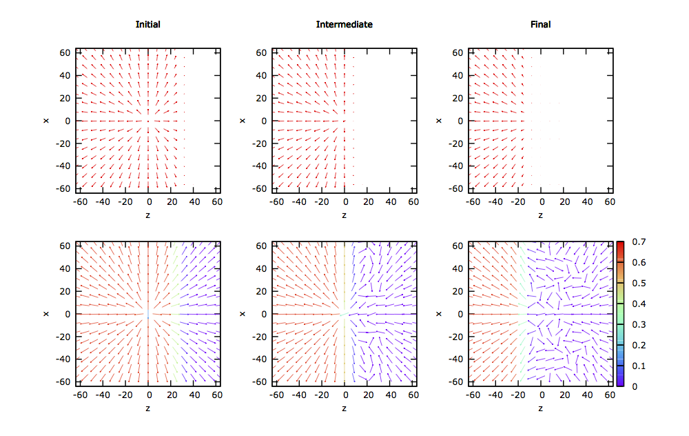
In Fig. 7, we show the $a=1,2,3$ components of the scalar field using two different representations. In the first row, the fields $\phi^{3}$ and $\phi^{1}$ are plotted as a vector. The plot shows that the components of the field that are responsible for the winding vanish on the $z=+\infty$ side of the wall. In the second row of Fig. 7, the color represents the magnitude $|\phi|\equiv\sqrt{\phi^{a}\phi^{a}}$, $a=1,2,3$, while vectors are drawn of fixed length and direction given by $\tan^{-1}(\phi^{3}/\phi^{1})$. Even though $|\phi|$ becomes very small, it is not strictly zero at a finite distance from the wall, and so one can still define the direction of the arrow in this way. One can see that initially the field has a hedgehog configuration across the wall. However, as the wall sweeps along, the fields on the $z=+\infty$ side of the wall rotate around in such a way as to unwind the monopole. In the final step, all fields that are non–zero are pointing in one direction, and therefore the monopole winding is gone.