The Künneth formula for graphs
Abstract.
We define a Cartesian product for finite simple graphs which satisfies the Künneth formula and so for the Poincaré polynomial and for the Euler characteristic . The graph is homotopic to , has a digraph structure and satisfies the inequality and . Hodge theory leads to the Künneth identity using the product of harmonic forms of and . A discrete de Rham cohomology and “partial derivatives” emerge on the product graphs. We show that de Rham cohomology is equivalent to graph cohomology by constructing a chain homotopy. The dimension relation holds point-wise and implies the inequality , mirroring a Hausdorff dimension inequality dimension in the continuum. The chromatic number of is smaller or equal than and . Indeed, is the maximal for which there is a subgraph of . The automorphism group of contains . If and are homotopic, then and are homotopic, leading to a product on homotopy classes. If is -dimensional geometric meaning that all unit spheres in are -discrete spheres, then is -dimensional geometric. And if is -dimensional geometric, then is geometric of dimension . Because the product writes a graph as a polynomial of variables for which the Euler polynomial is and , the product extends to a ring of chains which unlike graphs is closed under the boundary operation defining the exterior derivative and closed under quotients with . By gluing graphs, joins or fibre bundles are defined with the same features as in the continuum, allowing to build isomorphism classes of bundles.
Key words and phrases:
Discrete Kuenneth, discrete de Rham, Cartesian product, dimension, chromatology, homotopy and algebraic topology for graphs1991 Mathematics Subject Classification
Primary: 05Cxx, 57M15, 55U10, 55N10

1. Introduction
As acknowledged by nomenclature, Descartes concept of coordinates depends on the notion of a Cartesian product.
Omnipresent in mathematics, it is already used in basic arithmetic to build number systems like
the field of complex numbers or to define exterior bundles on manifolds. The Cartesian product
allows to build and access higher dimensional features of geometric spaces. Many constructions
in topology like suspensions, joins, fibre bundles, de Rham cohomology or homotopy deformations would not
work without the concept of a Cartesian product. Of course, we would like to have a product in graph theory
which shares the properties from the continuum. The new graph product will achieve that.
It will allow to use “coordinates” similarly as they are used in the continuum.
For two arbitrary networks - that is and are finite simple graphs -
the coordinates of the product graph consists of all pairs of complete subgraphs of and .
The exterior derivatives in and will
play the role of the “partial derivatives” in the product and allow to build an exterior de Rham derivative
on the product graph . The actual exterior derivative on the product graph
operates on a much larger complex. The later is called the Whitney complex and is
defined by the simplices in the product.
Having a product allows to work with “rectangular boxes”s in the product space rather than with
simplices. Figure (1) illustrates this for a small example.
To take a picture from the continuum: the curl in the plane is an infinitesimal line integral along a rectangle
and uses the Leibnitz rule to relate the exterior derivative of the factors with the exterior derivative
of the product. A simplicial point of view of cohomology integrates around
infinitesimal triangles to get the curl, ignoring the product structure.
De Rham establishes equivalence of the two pictures
on any smooth manifold. In order to prove the Künneth formula, we will need to emulate the de Rham theorem
combinatorially. To do so, we explicitly construct a -form on the Whitney complex of
from a -form on the de Rham complex defined by the two graphs . The chain map is concrete as
we can from this construct explicit cohomology classes of the product from the cohomology classes in or .
The relation is what one calls a chain homotopy.
The de Rham picture will be useful if we work with “discrete n-manifolds” obtained by gluing together local charts of
products of networks or when working with “fibre bundles”
obtained by gluing locally trivial charts of networks above a discrete manifold
covered with charts . The automorphism group of the fibre will then play the role of a gauge group on
, as it does in the continuum.
When looking at graphs as geometric structures without dimension restriction,
an amazing similarity with the continuum emerges. It turns out that in the discrete, one can access
the local structure of space directly as the complete subgraphs of . These simplices
can serve as fundamental entities playing the role of “points”. Such insight has been promoted
already in [7] but most of the time still graphs are treated as one dimensional
simplicial complexes. An illustration on how the change of view point allows to emulate results from
the continuum is the fixed point theorem of Brouwer and Lefschetz which looks identical
to the result in the continuum [20].
Many concepts become elementary: cohomology is part of
finite dimensional linear algebra, to compute valuations, generalized volumes, one needs integral geometric
tools in the continuum, while in the discrete is is just count of complete subgraphs.
The discrete Hadwiger theorem [15] is much easier than the continuum version: the numbers of
-dimensional simplices is a basis for the linear space of valuations.
Differential forms are just functions on a simplex graph and Stokes theorem in the Whitney complex
is a tautology; it becomes only less obvious when Stokes is considered in a de Rham setup.
Much Intuition about higher dimensions can be obtained inductively. There are notions of
dimension, cohomology, homotopy, cobordisms, ramified covers, degree and index, spheres, geodesic
lines and curvature which lead to results mirroring the results in the
continuum. This is not only true for nice geometric graphs but for general undirected networks or finite simple graphs -
and much works without any exceptions.
The notion of homotopy of graphs for example immediately leads to the homotopy of a graph
embedded in an other graph and so to homotopy groups for general finite simple graphs.
The product defined here will actually help to define the homotopy groups as graphs might
be too small at first to have spheres embedded, so that the graph should
first be refined. But the Hurewicz homomorphisms
from the homotopy groups to the cohomology groups are then so explicit that one can
even watch it happen: just apply the heat flow to a
-forms with support on the -simplices on the embedded -sphere. It converges to a harmonic form which
by Hodge theory represents a cohomology classes. In the continuum, such a
proof requires de Rham currents, generalized differential forms which require some
functional analysis. In the graph case, the heat flow is just
a linear ordinary differential equation of the type studied in introductory linear algebra courses.
The definition of homotopy groups which are relevant in coloring questions for graphs
[25, 28]
allows to work with spheres in graph theory in the same way as in the continuum.
The Euclidean product is not only essential for defining fundamental objects like fibre bundles,
it is also needed to construct spaces which have the same properties than classical manifolds.
Examples of such properties are dimension, homotopy, cohomology or Euler characteristic.
The goal of this note is to give such a product, allowing the use tools like discrete fibre
bundles in graph theory. We will see that this can be done purely algebraically:
as we can glue graphs together, this gluing carries over to the product allowing to build discrete bundles.
And if the fibres carry an automorphism group , we get discrete analogues of principle
bundles on which an enlarged gauge group acts.

A Cartesian product for a category of a geometry needs to be dimension-additive, it needs to
induce a product on the homotopy classes, it needs to be Euler characteristic multiplicative,
it must satisfy the Künneth formula equating
the tensor product of the cohomology rings with the cohomology ring of the product and it must have the property
that the automorphism group contains the automorphism groups of the factors.
As for graphs, no previously defined product shares these properties. The standard Cartesian product of the cyclic graph with for example is a graph of dimension . Its vertices are the Cartesian product of the vertices and two points are connected, if or . The cohomology of the standard Cartesian product has little to do with the cohomology of the factors: the Betti numbers of for example is while the Betti number of our product is , which is identical to the one of the two-dimensional torus in classical topology. The dimension of the traditional product is while the dimension of our product is .


Also other constructions like the “tensor product”, the “direct product” or the “strong product” of graphs do not have the topological properties we want. The reason for the shortcomings of all these products is that they do not tap into the lower dimensional building blocks of space: these are the simplices = complete subgraphs in the graph case. What in the continuum has to be done with sheaf theoretical constructs, is already pre-wired in the graph as we can access the lower dimensional simplices as “points”. The new product has the property for example that is a -dimensional torus of Euler characteristic and Betti vector . It is a triangularization of and each unit sphere is a -dimensional sphere of Euler characteristic . The product has practical use as it allows to construct high dimensional geometric spaces from smaller dimensional ones. The product works for any pair of graphs and leaves geometric -dimensional graphs invariant, graphs for which all unit spheres are -dimensional homotopy spheres defined in [28]. The product will again have this property. Cohomology, dimension and homotopy properties of the product are identical to the properties in the continuum. Even in the case of fractal dimension, the dimension formula matches the corresponding product formula in the continuum [6] (formula 7.2) for the Hausdorff dimension of arbitrary sets in Euclidean space. There are more analogues: for Hausdorff dimension, there are sets of dimension zero for which the product has dimension . While graphs of dimension are geometric, so that one gets equality, there are sequences of graphs like for which and , mirroring the continuum again.
An other useful feature of the product is that it allows to
refine graphs: the enhanced graph is a barycentric refinement of and this can be repeated:
the sequence produces a finer and finer mesh whose dimension converges
to an integer and honor the original symmetries if is a subgroup of the automorphism
group then still acts on the refinement. The later is important when looking at discrete principal bundles.
Moreover, while is in general no more a graph, the quotient is, so
that we can as in the continuum form covering spaces ramified over rather general
subgraphs. For example, while acting on has a quotient which is only a chain and no more a finite simple
graph, the quotient is a graph. As an other example, the quotient
of the octahedron modulo the action given by the antipodal reflection group
is no more a geometric graph without boundary as it is the wheel graph for which we can
see the octahedron as a double cover ramified over the equator (Riemann-Hurwitz in the discrete
is just the Burnside lemma considered simultaneously for the various simplex sceletons as noted
in [30]),
but is a geometric graph, a discrete projective plane.
As unit spheres of geometric graphs are spheres, the product can be used to construct new spheres. By taking refinements and then
taking quotients, one can get more general discrete graphs like the projective plane in the simplest case.
The product construction can also help for other constructions, like constructing joins or building discrete Hopf fibrations
in arbitrary dimensions. As every unit sphere in the product has the structure which is the union of two solid tori glued along the torus .
In the case when taking the product of -dimensional geometric graphs, we get so -dimensional
spheres which have naturally the same Hopf fibration structure as in the continuum.
Classically, the notion of a homotopy of two continuous maps is defined using the product:
if there is a continuous map , such that and , then
are called homotopic. This could be done now also for graphs: two graph homomorphisms are
homotopic, if there exists a line graph and a graph homomorphism from to such
that and . We have suggested in [25] an other definition:
two graph homomorphisms are homotopic if the “graph of the graph homomorphisms” are homotopic
graphs. These graphs of homomorphisms have as vertices the union and as edges
all pairs and pairs with .
Two graph homomorphisms are now homotopic, if the corresponding graphs are
homotopic as graphs. We believe that these two definitions are equivalent, but have not yet proven this.
In any case, we have the Whiteheads theorem that if there is a graph homomorphism which induces
isomorphisms on homotopy groups , then are homotopic. And as in the
continuum, having isomorphic homotopy groups does not force a homotopy equivalence. Now, with a product
we can take the same standard counter example and , where are
graph implementations of the -dimensional projective space and are -spheres. Since they have the
same universal cover and the same fundamental group , they have the same homotopy groups
but the Künneth formula implies that the Poincaré polynomial of is
while the Poincaré polynomial of is . Having different cohomology groups
prevents the two graphs to be homotopic. We see in this example, how useful it is to have a product
in graph theory which shares the properties from the continuum. The point is that one does not have to
reinvent the wheel in graph theory but that one can piggy-pack on known topology.


From a practical point of view, the construction of the product only needs a few lines of code for a
standard computer algebra system. The full computer code is given in detail later on. The product
works for all finite simple graphs: first construct the ring elements
which are polynomial in representing the vertices of
and , the vertices of , then take the product and construct
from this a polynomial in the variables , the new graph by connecting two monomial
terms of a polynomial if one divides the other. For example, if then and if then
, we get which encodes a wheel graph with central
vertex represented by . We see that the product naturally extends to chains, group elements in the ring
and that it corresponds to the product in the tensor product of the two rings. Every
polynomial defines back a graph, but the later does in general not not agree with the original host graph.
For example, take and the chain element , which defines in turn a graph which is the
disjoint union of (represented by ) and represented by . Chains are useful constructs
because natural operations escape the class of graphs: examples are forming the boundary or
taking quotients with a subgroup of the automomorphism group of . Chains form a ring
and have properties wanted from a geometric object: a dimension, a cohomology, a notion of homotopy, an
Euler characteristic, a notion of curvature and these notions match the results we expect from the familiar cases:
Results like Gauss-Bonnet [16], McKean Singer and Hodge-De-Rham [19],
Poincaré-Hopf [17], Brower-Lefschetz [20],
Riemann-Roch ([1] is a strong enough theory so that it can be extended to higher dimensions),
integrable geometric evolutions [23, 22],
Riemann-Hurwitz [24], Lusternik-Schnirelmann [14],
mirror the results in the continuum. See also [21] for an overview from the linear algebra point
of view. These results are more limited, if one considered graphs as one-dimensional simplicial complexes only,
a common assumption taken in the 20th century.
As graph theory is a discrete theory, it can surprise at first that the situation parallels the continuum so well
but there are conceptual reasons for that, an example is non-standard analysis, an other is
integral geometry. Some notions go over pretty smoothly, like cohomology or homotopy: others,
like the notion of homeomorphisms for graphs needs more adaptations [27].
About the history: Künneth found the formula in 1921 [10],
where it was his dissertation under the guidance of Heinrich Tietze. The paper published in 1923
[32] is a linear algebra analysis which could probably be simplified considerably
using Hodge theory. Künneth attributes the Cartesian product of manifolds to Steinitz (1908)
(The definition is indeed given in [41] p.44 is probably the first appearance of the
simplicial product which our definition is based on).
The notion of manifolds was initiated by Poincaré (1895), Weyl (1912),
Veblen and Alexander [43] (1913) and Whitney [45] (1936).
It was Herbert Seifert who introduced fibre bundles in 1933 [39]. The Eilenberg-Zilber
theorem of 1953 [40]. (Joseph Abraham Zilber was a Boston born
Harvard graduate (1943) and PhD (1963). Interestingly, the Eilenberg-Zilber theorem
was authored 10 years before Zilber got his PhD degree under the guidance of Andrew Gleason.
More information about the history of algebraic topology, see [4, 38]
or the introduction to [34].
The classical Cartesian product of graphs was introduced by
Whitehead and Russell in Principia Mathematica 1912 (it is [12] who spotted the construction
on page 384 in Volume 2 of that epic work). It was introduced there in the context of logical relations,
not so much graph theory.
This historical observation and many properties of the classical product product are discussed in
[12].
As far as we know, our present paper is the first establishing a Künneth formula for finite simple graphs.
There is a functorial approach to Künneth for digraphs, where
[11] use path cohomology to get a functor from digraphs to CW complexes, so that
one can then use the continuum result for the CW complexes. Note however that in their case,
one gets Künneth only indirectly by constructing a CW-complex, take the product using the Cartesian
embedding and then pulling the result again to graphs. In particular, the notion of dimension is also
borrowed from the continuum as CW-complexes are topological spaces.
A similar thing could be done for geometric graphs, graphs for which the
unit spheres are homotopy -spheres. One can then build for each ball an open set
in and use this to build a manifold . The open sets form then a nice good cover and the
topology of the manifold is the same than the topology of the geometric graph. This construction is
restricted however to geometric graphs.
The missing Cartesian product bothered us for a while so that we decided to make a targeted search over several weeks (while procrastinating from an urgent programming job still in need to be finished in geometric graph coloring), trying several possibilities and checking with the computer whether the construction works. The product described here was obtained by trying random things which look “beautiful”. The current product is attractive when seen algebraically because it becomes associative on the algebraic level. Until now, we would just take the usual product and then fill out the chambers. When working with graphs, this is cumbersome, even when staying within the discrete, as it costs programming effort to build examples, like stellated higher dimensional cubes. The product which we propose here for graphs seems not to be known in the language of graphs. One could of course take the product of the corresponding topological spaces as Künneth did. After finding the product, we looked around whether it already exists: closest to what we do here appeared as an exercise in an algebraic topology course by Peter Tennant Johnstone at Cambridge [13]. More digging revealed that this simplicial product has been used by Eilenberg and Zilber in [40] (page 204), by De Rham [37] (page 191) and earlier by Steinitz in [41] (page 44). But this product never made it to graph theory. One could also get a product by escaping to the Euclidean space. Our reluctance to use Euclidean stuff is not because we feel like Brouwer (who would even refuse to accept the infinity of natural numbers), but simply out of pragmatism: we want to build the structures fast on a computer without having to use Euclidean parts. Graphs are natural structures built into computer algebra languages and the Euclidean embeddings are not needed, when doing computations; only if we want to see the graphs visualized or modeling traditional geometric objects, the Euclidean embedding is helpful. Here is a self-contained full implementation of the new graph product in “Mathematica”, a computer algebra system which uses graphs as fundamental objects in its core language, structures which are dispatched from Euclidean embeddings, unless they are drawn. One procedures allow to translate a graph into a ring element and an other allows to get from a ring element back a graph. The graph product is the product in the polynomial ring.

The code of the above listing can be grabbed by looking at
the source of the ArXiv submission of this text.
Can we write the usual product in an algebraic way? Yes,
if we have the ring element and take as vertices the -dimensional simplices and
as edges the -dimensional edges, we recover the old graph.
If we take the product and take as vertices the pairs and as edges
the triples , we regain the standard Cartesian product.
For example, if represents and
represents , then the quadratic and cubic terms
of are
give the product graph which has vertices and edges.
2. Construction
In this section, we describe that the vertices of a graph define a ring in which every element can be
seen as its own geometric object which carries cohomology, homotopy, Euler
characteristic, curvature, dimension and a Dirac operator. As we could run the wave or heat equation
on such a ring element , the chain should be considered a geometric object with physical context.
Unlike the category of graphs, the category of these
chains has an algebraic ring structure, is closed under boundary formation as well as taking
quotients which leads to orbifolds in the continuum. Other constructs in the continuum like
discrete stratifolds are already implemented as suspensions of geometric graphs and are represented by classical graphs.
We called them exotic in [28], where we asked whether they might lead to exotic discrete spheres
(a -dimensional graph with geometric unit spheres which is homeomorphic to a -dimensional homotopy sphere)
and looked at discrete varieties in [28].
Somehow, chains form are part of a list of class of structures which resemble structures in the continuum
geometric graphs stratifolds varieties graphs orbifolds chains.
The product goes all the way to chains and can also be used to lift the
classical Cartesian product to -dimensional chains: it is obtained by taking the
product and disregarding higher dimensional parts of the chain: kind of projecting the result onto curves.
We use multi-index notation .
A finite simple graph with vertices defines a ring
generated by all non-constant polynomial monoids
and the chain ring. With a given orientation,
graphs are always represented by functions of the form with
and . The star graph for example is .
The ordering of the terms in the monoid
allows in a convenient way define an orientation of the simplices in the graph which
means fixing a basis for discrete differential forms .
We could add constants to get a ring with but we don’t yet see a use of
the constants for now as we have no geometric interpretation for it. The Euler characteristic formula
shows that the Euler characteristic of is .
The element can’t be interpreted as the empty graph, because the empty graph is
represented by , and is a -dimensional sphere with Euler characteristic . With a element in the ring,
one can produce terms like , an
object of Euler characteristic or , an object of Euler characteristic .
To add an other footnote, we see that some chains represent already special differential forms, but these are
forms taking values in the integers. The triangle is a sum of a -form, a -form and
-form which are all constant .
In this discrete setup, geometric objects and differential forms are already very similar, as it is custom
for quantum calculus setups, where Stokes is just the statement
and where the boundary operation is truly the adjoint of the exterior derivative and both geometric objects and
forms are in the same function space. For classical differential forms and geometric objects,
the geometric objects are distributions (as curves and
surfaces for example are infinitely thin) and differential forms
are smooth or the dual setup used in geometric measure theory where differential forms are distributions and
smooth functions are geometric objects. Its only on the level where
both parts (geometric objects and differential forms) are represented by the same type of data that we have
true symmetry, but then we are in a quantum setup.
Every element defines a graph : the vertices of are the monomials of and two monomials of are connected by an edge if one is a factor of the other. The graph of for example is the union of a line graph with three vertices where represents the middle vertex, as well as a single represented by . The graph on the other hand defines the ring element , where is a simplex in . The choice of the sign or permutation when writing down the polynomial monoid components corresponds to a choice of basis and is irrelevant for most considerations like for computing cohomology or when running discrete differential equations like [23, 22].


After fixing an orientation for each simplex, we get
incidence matrices . They implement the exterior derivative. They also determine
the Dirac operator , and all such matrices are unitarily equivalent.
Independent of the basis is the form Laplacian which has a block decomposition into
Laplacians on -forms.
The enhanced graph is a refinement of and as we will see, if is geometric, then the refinement
is geometric again of the same dimension. For general networks we will show that the dimension
of can only increase, the reason being that higher dimensional parts will spawn off more “new vertices”.
For a triangle for example, the ring is and
. This ring element defines the graph for which the monomials
are the vertices. The divisor incidence condition leads to the
wheel graph which has the same topological features as . Of course, the refinement process can be repeated,
leading to larger and larger graphs with the same automorphism group.
The sequence of graphs define so larger and larger rings generated by more and more variables.
We will see that the dimension converges to an integer and that for large , the graph is close to a geometric
graph as the larger simplices will overtake all others. See Figure (11).
Given two graphs , define the rings ,
take the product in the tensor product of rings and translate that product ring element
back to a graph. The dimension of is defined inductively as plus the average of the dimensions
of the unit spheres and uses the foundation assumption that the empty graph has dimension .
A graph is geometric, if every unit sphere is a homotopy sphere. A homotopy sphere is a
geometric graph for which removing any vertex renders the graph contractible. Inductively, a graph
is called contractible, if there exists a vertex such that and
are both contractible, using the inductive assumption that the -point graph is contractible.
Homotopy can be defined algebraically. Inductively, a ring element is contractible if there
exists such that both ring elements
and are contractible.
The Euler characteristic of is , where is the number of -dimensional
simplices in . More generally, the Euler characteristic of a ring element is
. The Euler characteristic of the triangle for example is
. The Euler characteristic of the chain is .
The boundary of a ring element is defined as
, where are the usual partial derivatives and the result is
projected onto functions satisfying .
Due to the orientation assumption, this gives rise to sign changes. For example,
if the edges basis was chosen.
We have .
The exterior derivative on is defined as . As , we have cohomology groups
for any ring element. Let be the Betti numbers.
The Euler-Poincaré formula follows from linear algebra.
The boundary
is no more a graph in general. The star graph for example has
the boundary which is a chain.
The space of differential forms is a direct sum , where
is generated by functions supported on -simplices, polynomial monoid parts in the ring of degree .
Since are finite dimensional, the maps are represented by finite matrices.
They are called the incidence matrices and were considered by Poincaré already for triangulations
of manifolds.
The cohomology groups and more generally
are independent of the chosen signs, when defining the chain ring element .
The matrix is called the Dirac matrix of . Its square
is the form-Laplacian. It decomposes into matrices .
By Hodge theory, the dimension of the kernel of is the ’th Betti number .
Given a ring element and a monoid part in , its unit sphere is the unit sphere of in the
graph defined by . It consists of all monoids dividing or which are multiples of , without .
It is again a ring element.
The dimension is inductively defined as plus the dimension of the unit sphere.
The dimension of finally is the average of the dimensions of all monoids in .
The dimension of the triangle for example is
.
We have for example which defines the graph of dimension
and which is a line graph of dimension etc. We see that the dimension of the triangle is .
Of course, in the graph case, the dimension can be better computed on a graph level. The point is that the
dimension extends to a nonnegative functional on the entire ring in such a way that the average of the
dimensions of unit sphere of a monoids or generalized vertices of is the dimension of minus .
We also need an inner product on which is defined as
. It obviously satisfies all properties of
an inner product and especially defines a length .
Of course, the incidence matrices are adjoint to each other with respect to this product.
As graphs are special functions, we could use the inner product for example to define an angle
between two graphs on the same vertex set it is the of the fraction
, where is the number of common
simplices of and is the square root of the number of simplices in .
Lets summarize the main point:
Proposition 1.
a) Every graph defines a ring element , a sum over all complete subgraphs of .
b) Every element defines a graph
, where are the monoid entries in , with and where two entries are connected
if one divides the other.
c) If comes from a graph , then is a graph for which the original simplices are the points and
which has the same topological features than and which additionally has a natural digraph structure.
In other words, there is a functor from the ring to the
category of directed graphs given by the division properties (even so we often forget about the
directions) and that there is a second functor from the category of undirected graphs to
the ring. They are not inverses of each other but the cohomology agrees.
For other functorial relations, see the recent paper [11].
Remarks:
1) Every ring element also defines its own geometric object which has Euler characteristic, cohomology, dimension,
homotopy as well as curvature.
2) When forgetting about the anti-commutativity within the graph which is irrelevant for the graph product,
the ring could be replaced with a more general integral domain. It would allow to
see the graph product as an element in where .
This possibility can be useful when studying fibre bundles as one can work in a ring of the fibre graph.
3) The fact that the product of two graphs is obtained by writing the graphs algebraically using different generators
and producing from it again a graph:
is not unfamiliar to us. If we take the Cartesian product of two spaces, we use different variables for the different
directions. If we don’t take new variables and take in the ring, then this is in general a chain.
For a triangle for example, we get (using )
the chain . The graph which belongs to this chain is the star graph
as is the central vertex and the others the outer points (as they divide the central point).
The imposed Pauli principle imposed by anticommutativity
is irrelevant for the Euler characteristic, both for chains as well as for the graphs
derived from the ring elements .
4) The graph can be seen as a self-cobordism of with itself as it is a graph of
one dimension more which has two copies of as boundary. It is in general true that any geometric
graph is self cobordant to itself as we can sandwich two copies with a completed dual graph .
but for we don’t have to work on a construction. It is given.
5) Denote by the projection onto the linear subspace generated by until -dimensional
simplices. As pointed out before, we can recover from by building and then
building which is . With , then is the classical standard
Cartesian product of and .
3. Some geometry
The results for the graph product mirror results in the continuum. First we look at some basic constructions which deal with the notion of homotopy sphere or simply -sphere in graph theory. The definition of a -sphere in graph theory is recursive: a -sphere is a -dimensional geometric graph for which every unit sphere is a -sphere and such that after removing any of its vertices, we get a graph which is contractible. A -ball is a -dimensional geometric contractible graph with boundary which has a -sphere as its boundary. We call the interior of a ball the part of which is not in the boundary. A suspension of a graph is the join , a double pyramid construction: add two new points and connect the points to all the vertices of . A pyramid construction itself is the join . From the Cartesian product, we have construct joins by just building a product and identifying some variables in the algebraic representation of the graph. Examples are given at the end.
Lemma 2 (Suspension).
The join of a -sphere is a -ball. The suspension of a -sphere with a -sphere is a -sphere.
Proof.
a) By definition, the boundary of is which is a sphere. Also, the graph is
contractible.
b) Removing the second point produces the ball by a).
∎
Remark:
1) More generally, as in the continuum, and shown below,
the join of two spheres is a sphere .
2) Also as in the continuum, the definition of the join needs the product as the join is a quotient
of . It generalizes that the 3-sphere can be written as , which has an
interpretation of gluing two solid tori along a torus.
Examples:
1) The wheel graph is a 2-ball. It is the join , where
is the cyclic graph with vertices.
2) The -dimensional cross polytope is , where we have
factors. The square is equal to , the octahedron is etc.
Lemma 3 (Glueing ball).
Assume are -balls with boundaries and assume that is a ball with boundary . Then is a -ball with boundary .
Proof.
This is proven by induction with respect to . There are four things to show:
a) is contractible.
b) every unit sphere in the interior of is a -sphere.
c) every unit sphere in is a -sphere.
d) when removing a vertex from , we get a contractible graph.
For a) take a point in . We can retract everything in to .
For b) we only have to look at a vertex in . The unit ball decomposes
For c), we only have to look at a vertex in and see whether its unit sphere in
is a homotopy sphere. For d), we can retract a pointed part to .
∎
The next statement is the discrete analogue of the classical statement that the boundary of the product of two balls is a sphere and that it can be written as as which is the union of two solid tori glued at a torus. Also in the discrete, we can use the intuition from the continuum:
Lemma 4 (Cylinder lemma).
If are -balls with -spheres as boundary, then is a -sphere provided .
Proof.
Use induction with respect to dimension. The union is a graph of dimension . A unit sphere is in or whose intersection is . ∎


Examples:
1) If are two line graphs with boundary , then is
a union of two line graphs. Similarly is the union of two
line graphs. The union is a square, the intersection consists of the four
points .
2) If is a ball with -dimensional sphere and
is a -dimensional ball with -dimensional sphere , then
is the mantle of the cylinder and
are the top and bottom cover.
3) If is -dimensional and is -dimensional, then
is a -sphere.
4) If are two-dimensional balls, we can see
is the union of two
solid tori glued along a -torus. This Hopf fibration is
classically given as the split of
into two solid tori
and intersecting in the -torus .
4. De Rham cohomology for graphs
Among various other flavors of cohomologies, there are three equivalent cohomologies for
compact -manifolds: simplicial cohomology, de Rham cohomology and
Čech cohomology. For simplicial cohomology,
the manifold is triangulated into finitely many -simplices leading to a differential complex.
In de Rham cohomology, one works with the complex of differential forms, partial
derivatives tap into the local product structure of the manifold,
for Čech cohomology, the manifold is covered with a finite cover of open sets so that the
nerve graph determines the cohomology.
Each of the these cohomologies have advantages over the others: simplicial cohomology
is the computer science or combinatorial point of view which sees space as a mesh of small simplicial building blocks,
the de Rham cohomology is the analysis or calculus approach, which taps into the bag of techniques used
in calculus. In this flavour, the basic building blocks are cubes obtained from a local product structure
and the different directions are accessed with partial derivatives which we think of the exterior derivatives
in each factor. The Čech cohomology finally is the homotopy or topologal point of view which relies
on the fact that cohomology is more robust and transcends dimension. Simplicial cohomology is
straightforward and the simplest. De Rham cohomology requires local charts which are products
and taps into the differential structure of the manifold, allowing for an efficient computation of cohomology.
Čech cohomology finally is a flexible variant which illustrates best the homotopy invariance of
cohomology. It also can lead to considerable complexity reduction as on can for example retract a
space to a much smaller dimensional set. A solid torus for example can be retracted to a circle.
The equivalence of simplicial cohomology with de Rham cohomology is due to
de Rham. Later proofs of this theorem use the equivalence of Čech cohomology with
simplicial cohomology.
All three cohomologies have analogue constructions in graph theory. It is our goal to introduce
the analogue of de Rham cohomology and give a discrete analogue of the de Rham theorem. Of course
de Rham cohomology emerges only in the discrete if one has a product which is compatible.
The simplicial cohomology of a graph is the clique cohomology of using the Whitney complex
of all complete subgraphs. It is the oldest and has already been considered by Poincaré, even so
not in the language of graphs.
The Čech cohology is the cohomology of the nerve graph of a good cover,
where “good” in the discrete means that the nerve is homotopic to . Čech cohomology has
first been considered for graphs in [27], a paper which proposes a notion of what
a continuous map between graphs is, which is more tricky than one might think at first,
as classical topology badly fails as the topology generated by the distance is discrete
making it unsuitable. What is important for a good notion of continuity is to merge homotopy with dimension.
The equivalence of discrete Čech cohomology with discrete simplicial cohomology is there by definition
just relying on the fact that homology is a homotopy invariant.
What was missing so far in graph theory is an analogue
of de Rham cohomology, where “cubes” rather than “simplices” play the fundamental role. But one can not
really look at a de Rham cohomology for general graphs, if one does not have a Cartesian product for which
there is compatibility.
A de Rham type cohomology has been mentioned in [11], where a generalized path cohomology
introduced by [8] is considered for digraphs.
As their approach uses a functor from graphs to CW complexes and pulls back results from the product of
CW complexes to digraphs, there is no relation with what we do here. Other takes on discrete de Rham cohomology
study discrete notions for numerical purposes [42] or [2].
Our approach to de Rham cohomology is purely combinatorial and restricted to finite constructions.
As in the continuum, the de Rham complex for a product graph
can use some derivatives also in the discrete, but this is merely language:
while in simplicial cohomology, we write
for the boundary of a simplex
in the de Rham approach, we can write in the algebra
which is the same thing. It just uses the derivative notion in a formal way.
The de Rham connection will be needed in the Künneth connection, where we
look at the kernel of form Laplacians. Künneth will then be quite obvious. Without linking de Rham with
simplicial cohomology the relation is nontrivial, as the dimension of the space of differential
forms on the product graph is much larger than the product of the dimensions of the space of differential
forms on the factors. Already Künneth had to work though such difficulties and needed dozens of pages
of linear algebra reductions to tackle the issue. Our situation is also different in that we look at the
product of two arbitrary networks which by no means have to be geometric.
The analytic de Rham approach allows the derivative to be written
as a sum of products which is Leibniz formula and which reduces the exterior
derivative of the product to the exterior derivative of the factors in the same way than
the gradient, curl or divergence reduces the exterior derivative to partial derivatives, which are the
exterior derivatives in the -dimensional factors. To illustrate this with school calculus:
infinitesimally, the curl of is . As a graph theorist we look
at (for fixed ) as the -form restricted to the first coordinate which means a function
on edges of the first graph and at (for fixed ) as the -form restricted to the second coordinate
which corresponds to edges in the second graph. The curl is so a line integral along
a square. When reducing this to simplicial cohomology, the square needs to be
broken up into triangles. Our product does that very explicitly even so it needs some care as the
tensor product of finite dimensional algebras has a completely different dimension in general
than the Cartesian product. Künnneth needed dozen of pages of rather messy linear algebra reductions
to achieve this. The language of polynomials and the de Rham connection
will allow us to make this more clear.
When we start with a triangulated picture, there are no more two distinguished directions
present. In graph theory, we only can distinguish two directions if we look at the product of two graphs.
As for manifolds, this structure could be allowed to be present locally only; its important however
that a product structure must be present
before we can even talk about discrete de Rham cohomology. As mentioned before, there is the possibility to see a
graph as a triangularization of a manifold and use the Euclidean product structure to emulate a discrete de Rham
cohomology. Notice however that this does not tickle down to the discretization. The relation would only
exist functorially and is pretty useless when working with concrete networks.
We will not leave the discrete realm and show that -forms on the product space can be related to
products of forms in the two factors. And also, we do not only work with geometric graphs,
which can be seen as discretizations of manifolds; we work with general finite simple graphs.
A finite simple graph naturally comes with a simplicial complex, given by the set
of all the complete subgraphs of . This so called Whitney complex can be
encoded algebraically in the ring of polynomials. For a triangular graph for example, we have the
ring element , where the choice of the orientations of all the
simplices is done arbitrarily. The ring element in turn defines a new graph
in which the polynomial monoids form the vertices and two vertices are connected
if one divides the other. It is important that it actually can be seen as a digraph,
the direction is given which part is a factor of the other. In some sense, going from to
frees us from having to chose an arbitrary orientation as the structure is now built in. By the way,
appears to have other nice features like having the Eulerian property allowing therefore a
geodesic dynamical system [28].
In our triangular graph example , we get a graph with
vertices because there are complete subgraphs of the triangle.
The graph is a wheel graph which shares the topological and cohomological
properties with the triangle. It is even homeomorphic to the triangle in the sense of [27]
as we can find a -dimensional open cover whose nerve is the triangle. Indeed:
the Čech cohomology of is equivalent to the graph cohomology of .
The observation that and are homotopic proves that the Čech cohomology
of a graph with respect to a good cover in the sense of [27]
is the same than the graph cohomology. As in the continuum, the relation between simplicial and
de Rham cohomology is not completely obvious as we will just see.
Now, if we take the product of two graphs, like for example two complete graphs
(illustrated in Figure (8)),
where the ring elements and encode the graph, then the product
is encoded by a ring element which by looking at
division properties of the polynomial monoids produces the graph with
elements. It is the wheel graph , which is a discrete square
with edges and triangles. The Laplacian
with the usual exterior derivative is a block matrix decomposing into
a block , a block and a block .
The algebraic representation of is a polynomial element with
monoid terms. The graph associated with would have vertices already.
From topological, algebraic or homotopical considerations, the graphs and
are equivalent: they are homeomorphic, they are homotopic and have the same cohomology
and dimension.
A boundary on the product is defined by the Leibniz formula:
which then defines an exterior derivative .
As for Čech cohomology, we will see that there is an advantage in that we can work
with a smaller dimensional vector spaces: the spaces and
and even the tensor product have in general
smaller dimension than the vector spaces . See Figure (1).
Having equivalence of cohomology can be a blessing when doing computations.
This will be useful when looking at discrete manifolds:
De Rham cohomology can be used more generally also
when gluing product graphs to build fibre bundle, this product structure
does not have to be global. It is the same situation as for
manifolds have in general only locally neighborhoods which can be written
as products.

Theorem 5 (Discrete De-Rham Theorem).
The de Rham cohomology for a product graph with boundary operation defined by the Leibniz rule using the exterior derivatives on each factor and , is isomorphic to the cohomology on defined by the exterior derivative on the graph . In short,
After de Rham [37], new proofs of the de Rham theorem in the continuum were given by A. Weil (1952) [44] and H. Whitney [46]. Weil had outlined a proof already in 1947 in a letter to H. Cartan, a letter which initiated Cartan’s theory of sheaves. Weil’s argument used a staircase argument in a double complex. The textbook proof of Bredon [35] is worked out in more detail in [35]. See also [36, 3, 9]. In the discrete, we can directly construct the chain maps and . As we will see below, our goal will be to find a one-to-one correspondence between harmonic forms on the large simplex Laplacian , which is a matrix and the de Rham Laplacian , which is a matrix. This is done by a rather explicit chain homotopy.
Proof.
Assume have vertices and .
The de Rham cohomology on the ring generated by functions
is defined by using the exterior derivatives on each
product using the Leibniz rule. We have to relate it with the Whitney chain complex
which features functions on the simplices of .
The linear spaces and
have different dimensions and
so that is not the inverse of (they are chain homotopic only, which essentially means that
they are equivalent modulo coboundaries on each side).
In both cases, denote by
and by the exterior derivatives.
We will construct two linear maps and check that they are chain maps:
and .
This will establish the isomorphism of cohomology
to .
Construction of :
Start with an -form . As it can be written as
in the variables , it defines a function
on the vertex set of . Given a -simplex in the graph
. Assigned to it the value of the vertex which belongs to a monomial
of degree . If there is one, it is unique. If there is none, assign the value .
Construction of :
For every -form in we
build a polynomial as follows:
the function defines a value to the vertices of
by averaging the values of the -simplices hitting . We have
now a function on the vertices of , written
as a polynomial in the variables .
One can now add a polynomial of smaller degree so that
can be factored as .
is a chain map: :
Proof: Given a -de Rham form , build the -form
using the Leibniz rule, then use to get from this
a -form on . By linearity, we can assume
that with . The function
takes the value on each polynomial with .
Now, is a -form on which takes the value
on those vertices . But is a form which assigs
the value to every simplex having as a vertex. Now
is exactly if is of the form .
is a chain map: :
Proof: given a -form on the product graph , we build
the -form and produce from this a polynomial in the de
Rham complex. We check that this is the same than .
by linearity we can look at a -form which assigns
the value to a simplex of . Now take a
-simplex which has in its boundary, then .
But now, assigns the value to the vertex which is in
and has degree . Now, assigns the value to
the vertex which is in and has degree . This is
connected to so that is the same value.
∎
It would be nice to have a more intuitive understanding of the function satisfying the chain homotopy condition
The map is related to the lower degree polynomial added to so that . This involves solving a system of linear equations. The dimension of the space of scalar functions on is , where is the number of simplices in . The space of functions has dimension . The image of consists of all lower degree polynomials (as usual satisfying ) which is a space of dimension . To solve for we have to solve a system of equations for variables and this solution gives us .

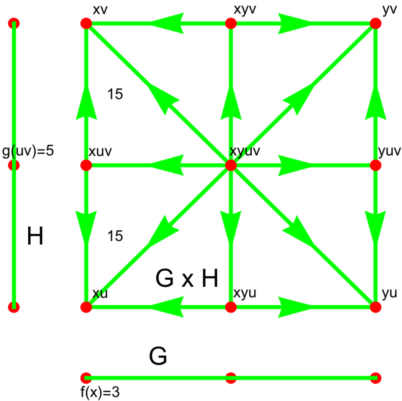
Examples:
1) If is a forest with trees and is a forest with trees,
then the product graph has components. The Betti vectors
are and . Every
harmonic form on the product space is of the form , where
are both locally constant. Because the number of vertices in
and -simplices in are the same, we don’t have to translate between
simplicial and de Rham -forms.
2) Let , then is a -dimensional ball with vertices
.
Given a -form in the product graph . It is a function on the
edges of . Given a vertex which is the product of a vertex and edge
like , we assign the sum over all edge values hitting the vertex.
Remarks:
1) In the complement of the set of chains which are
a product of graphs, the equivalence does hold any more.
Take the chain .
Its cohomology is different from the corresponding graph which is
the vertex graph without edges.
2) The graph of an abstract chain
has as many vertices as there are simplices in .
The simplicial complex of therefore is already large.
But the linear space of all -forms on
is huge: if is the number of simplices of and the number of simplices
in , then is the dimension
of the set of -forms on .
The de Rham complex is more manageable on a computer.
5. Results
Theorem 6 (Geometry of product).
If are geometric graphs of dimension then is a geometric graph of dimension .
Proof.
We have only to show that is a homotopy sphere. Depending on the graph is the union of two cylinders intersecting in a lower dimensional graph which is part of the sphere . Use the cylinder lemma. ∎
Corollary 7.
If are geometric spheres of dimension then the join is a geometric sphere of dimension .
Proof.
It is a graph of dimension as it is a quotient of a graph , where is a line graph with . This assures that for all points which are not affected by the identification, we have a geometric unit sphere of dimension . For the vertices which were subject of identification, the unit sphere is a union of two -dimensional cylinders which by the cylinder lemma is a sphere. Besides verifying that every vertex has a unit sphere which is a -sphere, we have also to check that taking away a vertex from , leads to a remaining graph which is a contractible ball of dimension which has a -dimensional boundary. ∎
Take . Given a vertex . It corresponds to a simplex in .
The set consists of all simplices in containing united with
the set of all simplices inside .
Examples:
1) Let be a cyclic graph . Lets look at the sphere of the vertex
which is now also a vertex in . It becomes now the set of two vertices in
corresponding to two edges in . This is a dimensional sphere.
2) Let again and let be an edge in which becomes now a simplex in .
Its sphere consists of the two simplices which correspond to two vertices in .
The sphere is , again a geometric graph.
3) In the case like if is an ecosahedron, assume that
is the old unit sphere of a vertex .
The new sphere of in contains the points which correspond to edges
in the old graph . The triangles are the new connections in that
sphere. We have again a geometric graph.
4) Now assume that is an edge in the old two dimensional graph which becomes
a vertex in . The sphere consists of the vertices which are the
third points in the triangles as well as the two triangles .
These two original vertices and triangles form 4 points in the new graph which form a
circular graph . This is our unit sphere.
5) Now assume that is a triangle in the two dimensional graph .
It becomes a vertex in the new graph . The unit sphere consists
of all simplices which is a -gon.
Examples 3)-5) together show that that is always geometric if is two dimensional.
The unit spheres always are and . In particular, is Eulerian.
6) In the case , if is an original vertex, then the sphere consists
of all edges and triangles in the original sphere by induction this is
. If is an edge. Then the sphere consist of the points
as well as all triangles and tetrahedra containing . This is a double
suspension of a -dimensional sphere and so -dimensional. If
is a triangle, then the unit sphere is a suspension of the -gon .
A theorem from 1964 assures that only spheres are manifolds which are joins
[33]. Since geometric graphs naturally define compact manifolds,
where unit balls are filled up to become the charts, this
holds also for geometric graphs. Intuitively, the reason is clear. In order
that the unit spheres of the identified end points are spheres, we better need
the factors of the join to be spheres, so that
is of the form where are spheres.
Corollary 8 (Kwun-Raymond).
If is a -dimensional geometric graph which is the join for two other graphs, then is a homotopy sphere.
Now, we come to the main result as announced in the title:
Theorem 9 (Künneth).
Given two finite simple graphs . The cohomology groups of are related to the cohomology groups of and by
Proof.
We know from Hodge theory that the de Rham Laplacian
of restricted to -forms has a kernel of dimension is .
We have and , so that
Hodge theory also assures that that is equivalent to , so that if
are harmonic forms in or respectively, then is a harmonic form in .
We see that we can construct the cohomology classes of the product
from the cohomology classes of the factors . It is obvious therefore that
contains the vector space .
Now assume that is harmonic in . We want to show that
or .
Again we use that the kernel of is the intersection of the kernel of
and the kernel of . Now look at the equation
where is a -form and is a -form. When we look at the terms, then
are polynomials in of degree and are polynomials in of
degree . But consists of polynomials of degree in and of degree in
and consists of polynomials of degree in the and of degree in . Because
the degrees are different, we see that .
Now, either which implies . But then,
so that also . An other possibility is which implies and in turn
implies . A third possibility is . But from
follows then .
Now take the inner product with to get which implies that , demonstrating that the
third case is not possible. We have seen that and and verified that every kernel element
in necessarily has to have the property that both and .
Having established that the de Rham cohomology of satisfies the Künneth formula
and that the de Rham theorem assures that it is equivalent to graph cohomology, we are done.
∎
Remark: In the continuum, the equivalence of the chain complex with the tensor product on which the exterior derivative is given by the Leibniz formula is subject of the Eilenberg-Zilber theorem from 1953 [40]. They use the nerve of product coverings and so Čech type ideas to verify the equivalence of the cohomologies and establish so the Künneth formula more elegantly. The above computation just reflects the fact that the tensor product of two chain complexes with exterior derivative given by the Leibniz formula is again a chain complex and that we have an Eilenberg-Zilber formulation as in the continuum, where two chain complexes are chain homotopic, if there are chain maps such that the composition is the identity and is chain homotopic to the identity in the sense that there is a linear map satisfying .
Corollary 10 (Eilenberg-Zilber).
Given two finite simple graphs . There is a chain map from to the chain complex and a chain map in the reverse direction such that and are chain homotopic.
Examples:
1) Let be the house graph and the sun graph . Both have the
Betti vector and the product has the cohomology of the -torus as it is homotopic
to the 2-torus. The graph has dimension , has vertices,
edges and triangles.
the graph has dimension and vertices and edges. The product
is a graph of dimension
. It has 120 vertices and 480 edges. The kernel of the Laplacian on -forms of
is spanned by ,
the null space of on -forms of is spanned by
. The Laplacian on the product graph is a
matrix. The Laplacian on the simplicial set is much smaller as it works
on a space whose dimension is the set of degree 3 monoids in which is .
2) The cohomology of has the Betti vector . The
cohomology of is .
3) The cohomology is the same as the cohomology of . Similarly, the
cohomology of the cylinder obtained by taking the products of a couple of
circles with the product of a couple of interval graphs is the same than of the torus
because the cube, the product of interval graphs is contractible.
4) The Betti vector of with is the k’th row
of the Pascal triangle . Easier to state, .
The reason for the following inequality is that higher dimensional simplices spawn more vertices in the graph . If the dimension is not uniform, then the dimension of the enhanced graph will increase. First of all, the construction of allows to define a local dimension for all simplices inside : it is just the usual dimension in the enhanced graph , where the simplices like are vertices.
Lemma 11 (Dimension inequality).
Given a finite simple graph . Then .
For , or any two point graph, we have equality. For all three point graphs different from the three point graph , we have equality too, while for we have a first inequality and . Denote by the dimension of the sphere in and by the dimension of the vertex in . The average of all these numbers is . We can not use induction as the unit spheres are not of the form with a smaller dimensional graph in general. However, we can do it with a chain. We therefore prove a stronger statement for chains : let the degree monomials be the vertices and the sphere of a vertex consist of the sum of degree monomials in which contain divided by . The small dimension of a chain is now recursively defined as the average of the small dimensions of the unit spheres of the vertices. The large dimension of the chain is the usual dimension of the graph . For a chain which comes from a graph , the small dimension is the dimension of , the large dimension is the dimension of which is the average over all large dimensions of the unit spheres , over all vertices in . The dimension inequality follows from the more general statement:
Lemma 12 (Generalized dimension inequality).
If is a chain then .
Proof.
The more general statement can now be proven with induction with respect to a lexicographic ordering which looks first at the the number of variables appearing in the chain and then at the number of monomials. This is a total ordering so that induction works. Unlike for graphs, the unit sphere of a vertex is now a chain with one variable less for which we can look at the small and large dimension. Also the unit sphere of a simplex is a chain for which we can look at the small and large dimension. The unit sphere of a simplex has in general the same number of variables but less monomials. ∎
Example.
The chain has two vertices .
(A) Lets look at first: the unit sphere of is which has two vertices .
(i) The vertex in has the unit sphere which has no vertices so that has dimension .
(ii) The vertex in has the sphere ,
a chain with one vertex which has a -dimensional sphere so that has dimension ,
has dimension and has dimension in .
The dimension of the vertex is therefore .
(B) The unit sphere of in is which has no vertex so that has dimension .
(C) The chain has small dimension .
The two computations (A)-(C) show that .
The large dimension of the chain is the average of the large dimensions of the monomials in .
It is the dimension of a graph with 6 vertices and 11 edges. It has dimension
which is .
Remarks:
1) The inequality looks like the known inequality between Hausdorff dimension and
inductive dimension in the continuum. But we do not see any relation yet.
2) When iterating the refinement construction, we get a sequence of graphs
with a dimension which converges to an integer.
Lets elaborate on this remark a bit more. The largest simplex will be the seed which grows fastest and take over.
Proposition 13 (Refinement asymptotics).
Start with a finite simple graph and define recursively , then , if is the largest clique in .
Proof.
The dimensions can only grow or stay by the lemma. Since the dimensions are bounded by for all , the dimensions must converge to some value smaller or equal than . The limiting value is because the number of subgraphs of grows exponentially and the growth of that large geometric cluster formed by the union of the simplices takes over: the number of subgraphs of is dominated by of subgraphs of . ∎


We see that when starting with an arbitrary network, we asymptotically get to a geometric graph. This could be interesting if we look at a dynamical emergence of graphs through refinement or evolution. It would explain, why geometric and manifold-like structures with integer dimension appear naturally: the lower dimensional structures grow slower and are overtaken by the growth of largest structures which make sure that a larger and larger part of will be geometric. The geometric part grows fast like the novo-vacuum in Schild’s ladder where physics is described by “Sarumpaet rules” [5]. Egan’s novel starts with with the words: In the beginning was a graph, more like diamond than graphite.

The dimension of is not necessarily equal to the dimension of . For example, the dimension
of the lollipop graph is , the dimension of is is slightly higher.
While has a cover for which the nerve graph is , the dimensions don’t agree because
higher dimensional parts of contribute more to .
We have looked a bit at the statistics
and computed the difference
which is related to the variance of the dimension random variable on a graph.
See Figure (12).
The preservation of dimension is an essential ingredient of a graph homeomorphisms, as it is in the
continuum. It is no surprise that in the fractal case, we have the same inequality like
Hausdorff dimension: .
Note however that the equality
holds in full generality, for any finite simple graph. We use the notation
where is the unit sphere of the vertex in .
Theorem 14 (Dimension of product).
Given two finite simple graphs . The dimension of is equal to the sum of the dimensions of and . More precisely, the dimension of any vertex in the dimension is the sum of the dimensions of in and in :
Proof.
Use induction with respect to the sum of dimension. Fix and assume , so that and . We only have to show that the unit sphere of in has dimension so that has dimension . The sphere is the union of two graphs , which overlap in . The two graphs have both dimension and has dimension . Lemma: if two graphs have dimension and their intersection has dimension then has dimension . ∎
For example, if is the tadpole graph and is the house graph, then and . The product graph has dimension .
Corollary 15 (Dimension inequality).
If are finite simple graphs, then .
Proof.
We have and . The result follows from Theorem (14). ∎
Given a geometric graph . A subgraph of is called convex if between any two vertices in , there exists a shortest connection between which is inside . Note that shortest connections are not necessarily unique. The convex hull of a finite set of vertices in is the intersection of all convex subgraphs of which contain .
Theorem 16 (Topology).
a) If is geometric, then is homeomorphic to in the sense of [27].
b) If has no triangles, then is homeomorphic to in the classical sense of
topological graph theory.
Proof.
a) Assume the graph has dimension .
Let be the vertices of . We have to find a cover
of such that the nerve graph of the cover is the original graph . As
we look at the unit sphere in the original graph and build the
smallest convex hull in containing all the vertices of this sphere.
The intersection of two is -dimensional and nonempty if and only if
were connected in the original graph.
Note that according to the definition [27],
intersections which are lower dimensional do not count as
edges in the nerve graph.
b) The graph is a refinement, where every edge has got an additional vertex.
∎
Examples.
1) If then the are balls of radius in the new graph
centered at the original vertices. Two sets overlap in line graphs of
diameter if and were connected in .
Theorem 17 (Continuity).
If and are homeomorphic geometric graphs and is a third geometric graph, then is homeomorphic to .
Proof.
We use that and are homeomorphic and that and are homeomorphic. if is a cover of and is a cover of such that the nerve graphs of are the same and is a cover of , then we have a cover and of and . ∎
Remark: We don’t yet know whether this can be proven for arbitrary finite simple graphs. One
first has to show that in full generality that and are homeomorphic. This is not
yet done.
Let be a finite simple graph. Define the curvature of a simplex in as the usual curvature [16] of the vertex in the graph .
Theorem 18.
The simplex curvature satisfies the Gauss-Bonnet relation . The function is equal to the expectation when integrating over all colorings on the simplex graph.
Remark:
We have already a natural ”curvature” for a graph located on simplices, it is constant
on the even dimensional simplices and on the odd dimensional simplices. But this
has little to do with the usual curvature.
Now, we look at symmetries:
Lemma 19.
Given two finite simple graphs . The automorphism group is a subgroup of the automorphism group of .
Proof.
Each element of produces a permutation of the variables appearing in the algebraic description of . If is the algebraic description of using variables , then acts on by permutations of the elements and produces a symmetry of . ∎
Remarks:
1) The case with shows that
the symmetry group can become bigger.
2) If the vertices of form a group and
also the vertices of have this property then
the vertices of form a group, the product group.
Next we look at homotopy:
Lemma 20.
If and are two finite simple graphs and the subgraph of is homotopic to the subgraph of and is homotopic to and is homotopic to , then is homotopic to .
Proposition 21.
The graph is homotopic to .
Proof.
Use induction with respect to the size of the graph. Its true for . Given a graph with vertices. Add a new vertex to get a larger graph with vertices. The unit sphere is in . Now is a subgraph of . Let denote the simplices in , they are the vertices in . The graph has new vertices which were not in . Our induction assumption is that is homotopic to and since is a subgraph of also is homotopic to . But then the graph in generated by is homotopic to the graph in generated by . Now is a union of two graphs and intersecting in and is the union of two graphs and intersecting in . Use the lemma. ∎
Theorem 22.
Let be finite simple graphs. If are homotopic, then and are homotopic.
Proof.
Show it on an algebraic level: if is a homotopy step, then is a homotopy step on each fibre. ∎
It follows that the product defines a group operation
on the homotopy classes. This monoid defines then a Grothendieck group.
The Cartesian product also defines a direct sum on isomorphism classes of
vector bundles.
Example.
1) The product of two trees is contractible.
2) The product is never contractible.
Finally, lets look at the chromatic number .
Lemma 23 (Minimal coloring).
The graph satisfies
It is minimally colorable. If is the largest complete subgraph of , then .
Proof.
If is a vertex in , denote by the dimension of the corresponding simplex in . The function is a coloring because two adjacent vertices have different dimension. Because takes values from to if is the largest simplex in , the chromatic number is . ∎
Remarks.
1) We see that for graphs we can immediatly compute the chromatic number
by just looking at the largest clique.
2) For geometric graphs , this means that is minimally colorable
and therefore is Eulerian in the sense of [29]. For two dimensional
graphs, this is equivalent to Eulerian in the classical sense.
We can actually compute the chromatic number of any product graph :
Theorem 24 (Chromatic number of product).
If has a largest clique and has a largest clique , then .
Proof.
Again just look at the function . It is locally injective and is so a coloring. ∎
This result actually has the previous lemma as a corollary
because has the largest clique so that
.
Examples.
1 The chromatic number of a product of two trees is .
2 The chromatic number of is .
The chromatic number of is .
6. Examples
Example.
Let be the house graph and the Lollipop graph. We have and ,
. The graphs satisfy
and . The graph has dimension . The dimensions of
the individual points are given by the dimension spectrum
{ 1, 1, 1, 7/4, 2, 2, 2, 7/4, 1, 2, 1, 2 }.
The dimension spectrum of is the Cartesian product of these two
lists:
15/4, 15/4, 15/4, 4, 4, 4, 4, 4, 4, 4, 4, 4, 4, 4, 4, 4, 4, 4, 4, 4,
4, 4, 4, 4, 2, 2, 2, 9/2, 19/4, 19/4, 19/4, 19/4, 5, 5, 5, 19/4, 5,
5, 5, 19/4, 5, 5, 5, 19/4, 5, 5, 5, 19/4, 5, 5, 5, 19/4, 5, 5, 5,
19/4, 5, 5, 5, 11/4, 3, 3, 3, 9/2, 15/4, 19/4, 19/4, 4, 5, 19/4, 4,
5, 19/4, 4, 5, 19/4, 4, 5, 19/4, 4, 5, 19/4, 4, 5, 19/4, 4, 5, 11/4,
2, 3, 15/4, 4, 4, 4, 4, 4, 4, 4, 2, 19/4, 5, 5, 5, 5, 5, 5, 5, 3, 4,
4, 4, 4, 4, 4, 4, 4, 4, 4, 4, 4, 19/4, 5, 5, 5, 19/4, 5, 5, 5, 19/4,
5, 5, 5, 19/4, 5, 5, 5, 19/4, 4, 5, 19/4, 4, 5, 19/4, 4, 5, 19/4, 4,
5, 4, 4, 4, 4, 5, 5, 5, 5, 4, 4, 4, 4, 4, 4, 19/4, 5, 5, 5, 19/4, 5,
5, 5, 19/4, 4, 5, 19/4, 4, 5, 4, 4, 5, 5, 4, 4, 4, 19/4, 5, 5, 5,
19/4, 4, 5, 4, 5, 2, 2, 2, 11/4, 3, 3, 3, 11/4, 2, 3, 2, 3.
This list had been computed directly by computing the dimensions of each
unit sphere in . The Künneth formula tells that
has the Betti numbers again for .


Example.
1) For an octahedron , the ring element is is
.
The graph is a barycentric subdivision of of the same dimension.
For a geometric graph , the graph is geometric again.


2) Let be the octahedron, the product is a -dimensional graph. It is a discrete incarnation of the -manifold .


3) A triangle is given by . Lets take the product with represented by . It becomes a -dimensional graph.


4) The product of with is a -dimensional graph. It is a -dimensional ball of radius with one interior point and all other points on the boundary. The curvature of the interior point is , the curvature of nine of the boundary points are and three are . By Gauss-Bonnet, the sum of the curvatures is , which is the Euler characteristic of the ball.


7. Lose ends
Dimension:
What is the expectation of on the Erdös-Rényi probability space.
This random variable measures in some sense the distance from a geometric graph as for
geometric graphs, the value is zero. The value of is related to the variance of the dimension
spectrum, which is a random variable on vertices of . It would be nice
to quantify this more.
Hausdorff dimension:
Due to the analogy of results with Hausdorff dimension ,
one can ask whether there is more to it
and whether for any subsets of Euclidean space ,
there are sequences of graphs such
that and .
Curvature:
The construction gives a convenient natural curvature
on the simplices of a graph . Gauss-Bonnet holds as they add up to Euler characteristic.
It is also true that curvature is the average over all functions [18, 26]
What is the relation between the curvature of and ?
The example of shows that the product of two zero curvature spaces
can develop curvature. The case shows
that the curvature can become very negative.
Spectrum:
What is the relation between the spectrum of with the spectrum
of and ? We know that the Laplacians live on different spaces.
The eigenvalues appear to correlated to the eigenvalues , where
is an eigenvalue of and is an eigenvalue of .
Chromatic number:
The case shows that the chromatic
number can become smaller. The product of two
geometric graphs is Eulerian in the sense [29] which
shows that if is a geometric graph, then is Eulerian.
The map regularizes in some way as for geometric graphs, the unit
spheres of are Eulerian spheres. Of course, it would be nice to see a relation between the
chromatic polynomials and of and . It is not always true
that divides but it is often the case. For the graph for
example, and .
Now .
For , this chromatic fraction of the graph is
. Already for , the chromatic fraction is not a polynomial.
Here is more random example, where the chromatic fraction is a rational function
and not a polynomial is the graph with vertices and edges
for which
the chromatic fraction is only rational.
Still, the chromatic number is for both graphs.
With respect to the known relation , we have inequality for all graphs .
For complete graphs , both sides are ,
for trees, both sides . For geometric graphs, all graphs have the property that .
On the list of all connected graphs with vertices, we have equality , on the list of all
connected graphs with vertices there are a dozen
for which the chromatic number has dropped, the reason
always being a -cycle of chromatic number becoming -colorable after the refinement.


Constructing spheres:
What kind of spheres appear as intersections of unit spheres in
discrete tori with .
We have seen that they all are unions of solid cylinders glued along a torus.
Assume we have obtained a class of spheres like that. Now take the product of
such spheres and take again unit spheres.
We get a larger and larger class of spheres. Can one characterize them?
Similarly, we can ask what kind of spheres can be obtained by applying the
join operation to spheres, starting with a smaller class of spheres.
Determinant:
Can we say something about the complexity of the
product, where is the pseudo determinant [31].
If , then the complexities of
are and . The complexity of is already
.
The pseudo determinant of the Laplacian of is and of is .
The pseudo determinant of the Laplacian of is .
Homotopy classes:
If is homotopic to and is homotopic to , then
is homotopic to . The sum and product therefore
produces a sum and product in the ring of homotopy classes. The contractible ring
elements form a class representing the element. The empty graph is the element.
Since also is homotopic to .
Homotopy extends to the ring of chains. Define contractibility in the same way
by telling is contractible if there exists such that both and
are contractible where is the non-constant part of the polynomial where is replaced by .
The unit sphere is the unit sphere of the graph .
Homotopy is so defined algebraically as reduction steps with contractible or reverse steps.
Contractibility is defined for in a polynomial ring as the property that there is a variable such
that and are both contractible. For example a line graph is contractible
as and are both contractible. The cycle graph is not contractible.
Also all its unit spheres like or which represent two point graphs are not contractible.

Suspension and join:
The topological notions of “suspension” and “join” needs the Cartesian product.
The definition of a suspension of a graph is
.
Also in the graph case, it produces from a -sphere a -sphere.
More generally, the join of two graphs can be defined as
An obvious questions is whether results like the double suspension theorem
of Cannon-Edwards can be proven directly in
graph theory. It certainly is true, as one can see by building corresponding
manifolds from the graphs. But it would be nice to have a direct discrete proof.
The double suspension of a graph is . A homology
-sphere is a graph which is geometric of dimension , which has the Poincaré
polynomial but which is not a -sphere.
The discrete Cannon-Edwards
theorem tells that if is a homology sphere, then is a sphere. To prove this
within graph theory, one has to show that every unit sphere in is a -sphere
and that removing one vertex in produces a -ball, a contractible -dimensional
graph with dimensional sphere boundary.


Higher order curvature:
It is natural to inquire whether for -dimensional geometric
graphs , the higher order curvature produces
a Gauss-Bonnet result. This is not the case as for the octahedron , the graph
has a sum of the second order curvatures which is . The culprit are the degree
4 vertices.
The sequence of graphs .
What happens with defined recursivly by is
that the minimal curvature goes to , at least if is two dimensional.
It would be interesting to know how the
curvature spectrum grows
for higher dimensional graphs.
The numerics is tough as the graphs sizes explode exponentially. L
If , then the curvature spectra are ,
.
If , then .
Global De Rham:
We have constructed a chain homotopy between de Rham and simplicial chains.
If we define a discrete -manifold as a graph which locally can be wrtten as a product
of networks such that on the intersection
there are coordinate change graph homeomorphisms, then the
chain homotopy can be pushed through. We don’t even need the graphs to have to
be -dimensional, nor have they be to be geometric. The combinatorial
de Rham theorem allows to deal with such discrete manifolds more effectively
similarly as the continuum de Rham theorem does.
Moving frames:
While a full classical Hopf-Rynov theorem on graphs is impossible because of the finiteness of
any reasonable tangent space and therefore, a quantum flow is needed for a reasonable notion
of geodesic map, there is weaker discrete
Hopf-Rynov theorem which tells that under some conditions, there is a global unique flow which
locally minimizes length [28]. What is needed for a geometric graph
of dimension is an Eulerian condition which is equivalent to the graph being
minimally colorable with colors. In [28], we made a stronger
assumption and required all unit spheres to be projective in order to associate to an
incoming ray an outgoing ray. There is an other approach which implements a
“moving frame” idea of Cartan and works for all Eulerian graphs and in particular
with of if are geometric. It in particular does not need the projective
assumption. A discrete moving frame is a pair , where is a -dimensional
simplex containing . The frame propagation defines a geodesic flow in an Eulerian graph
without the need of a projective involution: it is described inductively with respect to
dimension: use the geodesic flow on the Eulerian unit sphere to
flip the frame on the sphere
to the anitpodal side , where either the simplex
or the vertex has maximal distance (both cases are possible as the example in Figure (27)
shows), then reflect the vertex along the face to a vertex
on the adjacent simplex . This propagation
defines a variant of a geodesic flow for which the simplex plays the role of the direction,
as well (if we keep track of the frame in the simplex) produces a parallel transport on the graph.
The point we want to make is that for all product graphs and more generally
for all discrete manifolds obtained by patching product graphs, where each factor is a
geometric graph, there is a canonical notion of geodesic flow and parallel transport.
In some sense, there is a unique Levi-Civita connection on such graphs.


References
- [1] M. Baker and S. Norine. Riemann-Roch and Abel-Jacobi theory on a finite graph. Advances in Mathematics, 215:766–788, 2007.
- [2] D. Boffi. A note on the de Rham complex and a discrete compactness property. Appl. Math. Lett., 14(1):33–38, 2001.
- [3] R. Bott and L. W. Tu. Differential forms in algebraic topology. Graduate texts in mathematics. Springer Verlag, 1991.
- [4] J. Dieudonne. A History of Algebraic and Differential Topology, 1900-1960. Birkhäuser, 1989.
- [5] G. Egan. Schild’s Ladder. Victor Gollancz limited, 2002.
- [6] K.J. Falconer. Fractal Geometry. Wiley, second edition edition, 2003.
- [7] R. Forman. A discrete Morse theory for cell complexes. In Geometry, topology, and physics, Conf. Proc. Lecture Notes Geom. Topology, IV, pages 112–125. Int. Press, Cambridge, MA, 1995.
- [8] A. Grigoryan, Y. Lin, Y. Muranov, and S-T. Yau. Homologies of path complexes and digraphs. http://arxiv.org/abs/1207.2834, 2013.
- [9] A. Hatcher. Algebraic Topology. Cambridge University Press, 2002.
- [10] O. Haupt. Hermannn Künneth zum gedenken. Jahresbericht der Deutschen Mathematiker Vereinigung, 78:61–66, 1976.
- [11]
A. Huang and S-T. Yau.
On cohomology theory of (di)graphs.
http://arxiv.org/abs/1409.6194, 2014. - [12] W. Imrich and S. Klavzar. Product graphs, Structure and recognition. John Wiley and Sons, Inc. New York, 2000.
- [13]
P. T. Johnstone.
Algebraic topology examples 3.
https://www.dpmms.cam.ac.uk/study/II/AlgebraicTopology/2011-2012/ATqns3.pdf, 2011. - [14]
F. Josellis and O. Knill.
A Lusternik-Schnirelmann theorem for graphs.
http://arxiv.org/abs/1211.0750, 2012. - [15] D.A. Klain and G-C. Rota. Introductioni to geometric probability. Lezioni Lincee. Accademia nazionale dei lincei, 1997.
- [16]
O. Knill.
A graph theoretical Gauss-Bonnet-Chern theorem.
http://arxiv.org/abs/1111.5395, 2011. - [17]
O. Knill.
A graph theoretical Poincaré-Hopf theorem.
http://arxiv.org/abs/1201.1162, 2012. - [18]
O. Knill.
On index expectation and curvature for networks.
http://arxiv.org/abs/1202.4514, 2012. - [19]
O. Knill.
The McKean-Singer Formula in Graph Theory.
http://arxiv.org/abs/1301.1408, 2012. - [20] O. Knill. A Brouwer fixed point theorem for graph endomorphisms. Fixed Point Theory and Applications, 85, 2013.
- [21]
O. Knill.
The Dirac operator of a graph.
http://arxiv.org/abs/1306.2166, 2013. - [22]
O. Knill.
An integrable evolution equation in geometry.
http://arxiv.org/abs/1306.0060, 2013. - [23]
O. Knill.
Isospectral deformations of the dirac operator.
http://arxiv.org/abs/1306.5597, 2013. - [24]
O. Knill.
Classical mathematical structures within topological graph theory.
http://arxiv.org/abs/1402.2029, 2014. - [25] O. Knill. Coloring graphs using topology. http://arxiv.org/abs/1410.3173, 2014.
- [26]
O. Knill.
Curvature from graph colorings.
http://arxiv.org/abs/1410.1217, 2014. - [27]
O. Knill.
A notion of graph homeomorphism.
http://arxiv.org/abs/1401.2819, 2014. - [28] O. Knill. Graphs with Eulerian unit spheres. http://arxiv.org/abs/1501.03116, 2015.
- [29] O. Knill. Graphs with Eulerian unit spheres. http://arxiv.org/abs/1501.03116, 2015.
- [30] O. Knill and T. Tucker. A riemann-hurwitz theorem in graph theory. Draft Notes, December 2012.
- [31] Oliver Knill. Cauchy-Binet for pseudo-determinants. Linear Algebra Appl., 459:522–547, 2014.
- [32] H. Künneth. Über die Bettischen Zahlen einer Produktmannigfaltigkeit. Math. Ann., 90(1-2):65–85, 1923.
- [33] K.W. Kwun and F. Raymond. Manifolds which are joins. Trans. Amer. Math. Soc., 111:108–120, 1964.
- [34] J. Milnor. Collected papers of John Milnor. IV. American Mathematical Society, Providence, RI, 2009. Homotopy, homology and manifolds, Edited by John McCleary.
- [35] M.A. Perez. The de Rham’s theorem. Lecture notes, University du Quebec, 2010.
- [36] V.V. Prasolov. Elements of Combinatorial and Differential Topology, volume 74 of Graduate Studies in Mathematics. AMS, 2004.
- [37] G. De Rham. Sur l’nalysis situs des variétés à n dimensions. Journal de mathématiques pures et appliqués, 10:115–200, 1931.
- [38] E. Scholz. The concept of manifold, 1850-1950. In History of Topology. Elsevier, 1999.
- [39] H. Seifert. Topologie Dreidimensionaler Gefaserter Räume. Acta Math., 60(1):147–238, 1933.
- [40] S.Eilenberg and J. Zilber. On products of complexes. Amer. J. Math., 75:200–204, 1953.
- [41] E. Steinitz. Beiträge zur Analysis situs. Mathematische Annalen, 7:29–49, 1908.
- [42] X-C. Tai and R. Winther. A discrete de rham complex with enhanced smoothness. Calcolo, 43:287–306, 2006.
- [43] O. Veblen and J.W. Alexander. Manifolds of n dimensions. Annals of Mathematics, Second Series, 14:163–178, 1912-1913.
- [44] André Weil. Sur les théorèmes de de Rham. Comment. Math. Helv., 26:119–145, 1952.
- [45] H. Whitney. Differentiable manifolds. Ann. of Math. (2), 37(3):645–680, 1936.
- [46] H. Whitney. Geometric integration theory. Princeton University Press, Princeton, N. J., 1957.