An Implementation Model for Interaction Nets
Abstract
To study implementations and optimisations of interaction net systems we propose a calculus to allow us to reason about nets, a concrete data-structure that is in close correspondence with the calculus, and a low-level language to create and manipulate this data structure. These work together so that we can describe the compilation process for interaction nets, reason about the behaviours of the implementation, and study the efficiency and properties.
1 Introduction
Interaction nets [6] offer a visual aspect to rewriting. Analogous to term rewriting systems, a specific system is defined from a user-defined set of nodes (cf. terms) and a user-defined set of rewrite rules. Nets are then graphs built from the set of nodes and rules are graph transformations. Interaction nets are therefore a specific, in fact very constrained, form of graph rewriting.
Interaction nets have been used as a programming language, an intermediate language, and as a target language for the compilation of other programming languages. In all these application areas, prototype implementations have been built to support the work, but they are often not documented. The purpose of this paper is to take a new look at the implementation of interaction nets. Specifically, we are interested in documenting the implementation process, and in particular showing a compilation of nets to a low-level language. We aim to build on the past experience and knowledge obtained from building other implementations, and make a new contribution to this investigation. Specifically, we define: a calculus that can represent and express results about interaction nets; a data-structure with a low-level language that corresponds exactly to the calculus; and a compilation of the calculus to this low-level language.
In addition to defining the above, an important aspect of this work is the compilation of interaction rules: the ability to implement rules efficiently will impact greatly on an implementation. The low-level language is close enough to machine code that we essentially get atomic operations so that we can understand the cost of an interaction. From a practical perspective, we get reliable, efficient implementations of interaction nets from this work. In this paper we provide the foundations for this work, and point out a number of directions that are currently being investigated.
A number of evaluators have been developed for interaction nets, and one of the first abstract machines was given by Sousa Pinto [10]. From another direction, a graphical interpreter in2 was proposed by Lippi [8] and it showed an aspect of interaction nets as a visual programming tool. Some evaluators have been proposed towards efficient computation, called INET [3] and amineLight [4]. Our approach is to build the simplest implementation model for interaction nets that we believe can be the most useful as well as providing the basis for more efficient (including parallel) implementations in the future. We shall give some evidence to support this claim in the current paper.
The next section recalls some background material, and in Section 3 we describe the new calculus. In Section 4 we give the data-structure that corresponds to the calculus together with a low-level language. We include also some notes about the compilation of nets into the low-level language. In Section 5 we evaluate the work, and give some directions for future work. We conclude the paper in Section 6.
2 Background

In the graphical rewriting system of interaction nets [6], we have a set of symbols, which are names of the nodes. Each symbol has an arity that determines the number of auxiliary ports that the node has. If for , then has ports: auxiliary ports and a distinguished one called the principal port. Nodes are drawn as shown in Figure1. A net built on is an undirected graph with nodes at the vertices. The edges of the net connect nodes together at the ports such that there is only one edge at every port. A port which is not connected is called a free port.

Two nodes connected via their principal ports form an active pair, which is the interaction nets analogue of a redex. A rule replaces the pair by the net . All the free ports are preserved during reduction, and there is at most one rule for each pair of agents. The diagram in Figure 2 illustrates the idea, where is any net built from . The most powerful property of this graph rewriting system is that it is one-step confluent—all reduction sequences are permutation equivalent.
There are many possible data-structures that can be used to represent interaction nets, for example single or double linked graphs. Agents have exactly one principal port, so we can use this to our advantage and represent nets as a collection of trees, and use a simple, single linked structure. Computationally the cost of evaluating a net is mostly due to the cost of the rewrite step: building the right-hand side of the rule; connecting the new net to the old one; freeing up the left-hand side of the rule (agents and in the diagram in Figure 2).
The goal of this paper is to build an implementation model, together with a calculus, that explains this process and allows the study of the cost of computation. Specifically, we provide a framework where we can focus on the compilation of rules where we can perform the above steps in the fewest instructions.
3 Calculus
It is possible to reason about the graphical representation of nets, but it is convenient to have a textual calculus for compact representation. There are several calculi in the literature, and here we review the Lightweight calculus [4], which is a refined version of [2].
- Agents:
-
Let be a set of symbols, ranged over by , each with a given arity . An occurrence of a symbol is called an agent, and the arity is the number of auxiliary ports.
- Names:
-
Let be a set of names, ranged over by , etc. and are assumed disjoint. Names correspond to wires in the graph system.
- Terms:
-
A term is built on and by the grammar: , where , , and are terms, with the restriction that each name can appear at most twice. If , then we omit the parentheses. If a name occurs twice in a term, we say that it is bound, otherwise it is free. We write to range over terms, and to range over sequences of terms. A term of the form can be seen as a tree with the principal port of at the root, and the terms are the subtrees connected to the auxiliary ports of . The term represents an indirection node which is created by reduction, and is not normally part of an initial term.
- Equations:
-
If , are terms, then the unordered pair is an equation. ranges over multisets of equations.
- Rules:
-
Rules are pairs of terms written: , where is the active pair, and is the right-hand side of the rule. All names occur exactly twice in a rule, and there is at most one rule for each pair of agents. We call the free names in parameters and write it as . All other names are bound.
- Configurations:
-
A configuration is a pair , where is a set of rules, a sequence of terms, and a multiset of equations. Each variable occurs at most twice in a configuration, and we extend the nomenclature of free and bound names from terms. The rules set contains at most one rule between any pair of agents, and it is closed under symmetry, thus if then . We use to range over configurations. We call the head and the body of a configuration.
Definition 1 (Names in terms)
The set of names of a term is defined in the following way, which extends to sequences of terms, equations, sequences of equations, and rules in the obvious way.
The notation denotes a substitution that replaces the free occurrence of by the term in . This extends to equations and configurations in the obvious way.
Definition 2 (Instance of a rule)
If is a rule , then denotes a new generic instance of , that is, a copy of where we introduce a new set of bound names so that those new names do not overlap with others already exists, but leave the free names (parameters) unchanged. Example: if is , then is , where is a fresh name.
The configuration represents a net that we evaluate using ; gives the set of active pairs and the renamings of the net. We write without when there is no ambiguity. The roots of the terms in the head of the configuration and the free names correspond to ports in the interface of the net. We work modulo -equivalence for bound names. The computation rules are defined below, and we use instead of when there is no ambiguity.
- Communication:
-
.
- Substitution:
-
where and occurs in .
- Collect:
-
where occurs in .
- Interaction:
-
where .
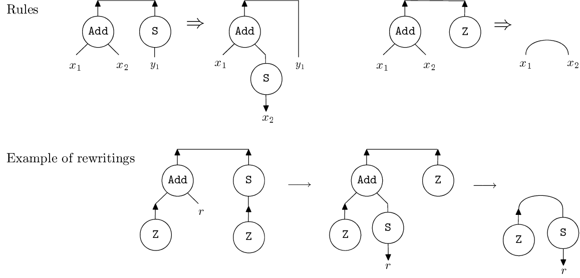
Example 3
Rules in Figure 3 can be represented as follows:
The net in Figure 3 is represented as , and it is performed:
We define by where is in normal form. The following theorem shows that all Interaction rules can be performed without using Substitution and Collect [4]:
Theorem 3.1
If , then there is a configuration such that and is reduced to by applying only Communication rule and Interaction rule.
We define by where is a normal form. Because all critical pairs that are generated by and are confluent, the determinacy property holds [4]:
Theorem 3.2 (Determinacy)
Let . When there are configurations such that and , then is equivalent to .
3.1 Simpler calculus
In Lightweight calculus, equations are defined as unordered pairs and configurations use multisets of equations. Here, in order to facilitate the correspondence between the calculus and an implementation model that has a code stack and an environment such as SECD-machine [7], we introduce another refined calculus of Lightweight one, called Simpler calculus, by changing the definition of equations into ordered pairs and in configurations multisets of equations into sequences of ones.
- Terms:
-
A term is built on and by the grammar: . Intuitively, corresponds to a variable bounded with (or a state such that an environment captures ).
- Equations:
-
If and are terms, then the ordered pair is an equation. will be used to range over sequences of equations.
- Rules:
-
Rules are pairs of terms written: .
- Configurations:
-
A configuration is a pair , where is a sequence of equations. The rules set contains at most one rule between any pair of agents, and it is closed under symmetry. We use to range over configurations.
Definition 4 (Computation Rules)
The operational behaviour of the system is given by the following:
| Var1: where . | Var2: where . |
| Indirection1: . | Indirection2: . |
| Interaction: , then | |
To remove indirection terms, we introduce an operation remInd (it is extended to sequences of terms and configurations in the obvious way):
These rules correspond directly to the graphical data-structure and operations given in the next section. Indirection is introduced so that the data-structure manipulations can be kept simple. However, there is an overhead of dealing with indirection nodes. Computationally the interaction rule is the most expensive: the other rules will turn out to be implemented with a small number of instructions or will be equivalences in the data-structure.
3.2 Expressive power
We compare the expressive power of Simpler and Lightweight calculi. We define a translation of configurations from Simpler calculus into the Lightweight one as: .
Lemma 6
Let and be configurations such that . When it is by Indirection1 or Indirection2 rules, . Otherwise, .
Proof 3.3.
In the case of Var1: . When we assume , then , and thus or .
Every equation is reduced by a rule in Simpler calculus, the following holds:
Lemma 3.4.
When , then is empty.
We define a translation of configurations ToSimple from Lightweight calculus into Simpler ones:
Theorem 3.5.
Let be a configuration in Lightweight calculus. When there is a configuration in Simpler one such that , then .
Theorem 3.7.
Let and be configurations in Lightweight calculus such that . Then there is a configuration in Simpler one such that and .
Proof 3.8.
If has no normal form, corresponding to an infinite reduction sequence from we can construct an infinite reduction sequence starting from by Lemma 6 since each reduction produces at most one equation such as or . This contradicts the assumption of this theorem. There is, thus, a configuration such that . By Theorem 3.7 , and thus there is a configuration such that and by Theorem 3.1. By the assumption and the determinacy (Theorem 3.2), .
We define a configuration of our abstract machine state by the following 3-tuple , where
- •
is an environment, which is a subset of ( is a set of names, is the set of terms),
- •
is an interface, which is a sequence of terms,
- •
is a sequence of equations to operate.
In contrast to the SECD machine [7], the stack , the environment and the control in the machine correspond to the term sequence , the map , and the equation sequence in this abstract machine respectively. There is no element corresponding to the dump in SECD machine because, during an execution of a rule, other rules are not called. To manage the environment, we define the following.
Definition 3.9 (Operations for pairs).
Let be a set of pairs.
- •
We define a map as a set of pairs: , otherwise.
- •
We use the following notations to operate maps:
- –
as a set for any ,
- –
as a set .
- –
We give the semantics of the machine as a set of the following transitional rules of the form by applying in the order from to :
Intuitively, the rule ‘A’ corresponds Interaction rule, ‘B1’ and ‘B2’ correspond Var1 and Var2, and ‘C1’ and ‘C2’ correspond Indirection1 and Indirection2. To force captured terms in the environment to be replaced when the execution is finished, we define Update operation:
4 Data-structures and language
![[Uncaptioned image]](1505.07164v1/diagram-config.png)
Here we give a low-level language, called LL0, which defines a set of instructions to build and reduce a net to normal form. The concrete representation of a configuration can be summarised by the diagram shown on the right, where represents the net, EQ a stack of equations, and I an interface.
For a net, we need two kinds of graph element: agents and names nodes. Each of these is allocated memory in the heap. An element, such as an agent, may contain pointers to other elements (representing auxiliary ports). An agent can be coded in C as follows:
typedef struct Agent {
  int id; struct Agent *port[];
} Agent;
In this Agent structure, each symbol for agents is distinguished by a unique id. The length of port corresponds to the number of auxiliary ports of an agent. The stack of equations EQ is initially empty. Intuitively, an element of this stack can be written using the following code fragment in C:
typedef struct Equation {
  Agent *a1; Agent *a2;
} Equation;
The interface I is a node arrays of fixed size as the size of the observable interface of a net can be pre-determined (and it is preserved during execution). By using LL0, we encode Simpler calculus.
Building nets.
Graph elements, the stack of equations EQ and the interface I are managed by instructions as shown in Figure 4. The port numbers start from 1, and by using the instruction , we can assign a graph node into a port of a graph node . We also use the port 0 to refer to the id of an element. For instance, changes the id of an agent node into .
| Instruction | Description |
|---|---|
| Declare as symbols of agents whose arity are . | |
| Create a fixed -size interface and assign its pointer to the variable I. | |
| Allocate (unused) memory for an agent node whose id is and assign it to the variable . | |
| Allocate (unused) memory for a name node, and assign it to the variable . | |
| Dispose of just an assigned allocation of a graph element (not recursively). | |
| Assign a graph element to a port of an agent node . | |
| Change the id of an agent node into . | |
| Create an equation of two graph element in the stack of equations. | |
| stackFree() | Dispose of the top element of the equation stack. |
![[Uncaptioned image]](1505.07164v1/agent_node1.png)
Here, we build terms in Simpler calculus. To assign an arity to an agent, we use the following declaration: , where is the arity for an agent symbol such that . After this declaration, a symbol can be represented by a unique number and an agent’s arity can be referred to by . We draw an agent node of arity 3 as shown the right above figure.
![[Uncaptioned image]](1505.07164v1/name-ind-node.png)
Name nodes are graph elements whose id is denoted by the symbol N and the arity is 0. We also use indirection nodes by $ and the arity is 1. We assume that N and $ are selected from a set that does not overlap with the set of agent symbols. To allocate an agent node whose id is to a variable , we use the following instruction: . A name node is allocated by . An assigned allocation of a graph element is disposed of (not recursively, just one node) by using .
A connection between a principal port and an auxiliary port is encoded by an assignment. In this language, to assign a pointer of an existing graph element to a port of another graph element , we use the following instruction: . We note that the index of these ports start from 1. For instance, a term Add(Z,r) is encoded as shown below, together with the graphical representation.
 1. #agent Z:0, Add:2
 2. aAdd=mkAgent(Add)
 3. aZ=mkAgent(Z)
 4. aAdd[1]=aZ
 5. r=mkName()
 6. aAdd[2]=r
![[Uncaptioned image]](1505.07164v1/agent_node_addzr.png)
![[Uncaptioned image]](1505.07164v1/tree.png)
Generally, when agent nodes are connected together, they are trees that we represent in the following way, where the free ports are at the top of the tree.
![[Uncaptioned image]](1505.07164v1/equation_node.png)
The stack of equations EQ is initially created empty. An equation node can point to two graph elements. To create an equation of two graph elements in the stack EQ, we use the instruction: . To pop an equation from the top of the stack EQ, we use the instruction: stackFree(). We represent a connection between principal ports by creating an equation between the two agent nodes into the stack.

Interfaces are created with the instruction: . Elements in I can be accessed using the usual array notation and can point to one graph element. As an example, a configuration is encoded using the instructions below. Figure 5 gives the corresponding data-structure. For a connection between two auxiliary ports, we assign one name node to two ports.
 1. #agent Z:0,S:1,Add:2
 2. /*interface*/
 3. I=mkInterface(1)
 4. /*Add(Z,r)*/
 5. aAdd=mkAgent(Add)
 6. aZ=mkAgent(Z)
 7. aAdd[1]=aZ
 8. r=mkName()
 9. aAdd[2]=r
10. /*S(w)*/
11. bS=mkAgent(S)
12. w=mkName()
13. bS[1]=w
14. /*Add(Z,r)=S(w)*/
15. push(aAdd,bS)
16. /*Add(Z,w)*/
17. aAdd=mkAgent(Add)
18. aZ=mkAgent(Z)
19. aAdd[1]=aZ
20. aAdd[2]=w
21. /*S(Z)*/
22. bS=mkAgent(S)
23. bZ=mkAgent(Z)
24. bS[1]=bZ
25. /*Add(Z,w)=S(Z)*/
26. push(aAdd,bS)
27. /*interface*/
28. I[1]=r
Defining interaction rules.
We introduce rule procedures to perform interaction rules. For an interaction rule between and we define a rule procedure using the syntax: and we write instructions between the brackets { and } (rule block). In execution, the procedures provide special variables that are pointers to the left and the right-hand side agents of the active pair equation. Variables used in the instructions are only visible within the rule procedure. Generally, these rule procedures are represented as transformations on the data-structure. For instance, the rule between Add and Z given by is represented using the following procedure:
 1. rule Add Z {
 2.   stackFree()
 3.   push(L[1],L[2])
 4.   free(L)
 5.   free(R)
 6. }
The following illustrates transformations that will be applied by the rule procedure given above.
![[Uncaptioned image]](1505.07164v1/encode_addz-1.png)
![[Uncaptioned image]](1505.07164v1/encode_addz-2.png)
In order to manage equations in the Simpler calculus, we need mechanisms that perform rules Var1, Indirection1 and so on. Figure 6 (a) and (b) are instances of Var1 and Indirection1 rules to illustrate this.
(a) where

(b)

Compilation of Simpler calculus into LL0.
Here we introduce a translation of Simpler calculus into LL0. We use a set of pairs and operations for the pairs defined in Definition 3.9. We also use a notation for strings. We write “ and ” as a pair of delimiters to represent a string explicitly. We use the notation in a string as the result of replacing the occurrence with its actual value. For instance, if and then . We use as an infix binary operation to concatenate strings.
Definition 4.1 (Compilation of terms and nets).
Here we defined our compilation schemes that will generate LL0 for a given interaction net system.
- •
We use a subset of ( is a set of names) so that a name can correspond to a string of a variable name in a code sequence and those correspondences can be looked up from compilation functions. We also use two operations and for as defined in Definition 3.9. We define a function makeN to make such a set and a code sequence for those names by a given name set . The function freshStr() returns a fresh name.
- •
We define a translation from a symbol set into a code string as follows:
- •
A translation from a term into a code string is defined as follows:
- •
A translation from an interface into a code sequence is defined as follows:
- •
A translation from an equation into a code string is defined as follows:
- •
A translation from an equation sequence into a code string is defined as follows:
- •
We define a translation from a configuration with a symbol set into a code string as follows:
- •
We write just Compile when there is no ambiguity.
Example 4.2.
Let us take a configuration with a symbol set as an example. The compilation generates the following instructions:
 1. #agent Z:0,S:1,Add:2
 2. r=mkName()
 3. a1=mkAgent(Add)
 4. a2=mkAgent(Z)
 5. a1[1]=a2
 6. a1[2]=r
 7. b1=mkAgent(S)
 8. b2=mkAgent(Z)
 9. b1[1]=b2
10. push(a1,b1)
11. I=mkInterface[1]
12. I[1]=r
Definition 4.3 (Compilation of rules).
We define a translation from a rule into a sequence of code strings as follows:
Example 4.4.
The results of and are as follows:
 1. rule Add Z {
 2.   stackFree()
 3.   push(L[1],L[2])
 4.   free(L)
 5.   free(R)
 6. }
 1. rule Add S {
 2.   stackFree()
 3.   w=mkName()
 4.   a1=mkAgent(Add)
 5.   a1[1]=L[1]
 6.   a1[2]=w
 7.   push(a1,R[1])
 8.   b1=mkAgent(S)
 9.   b1[1]=w
10.   push(L[2],b1)
11.   free(L)
12.   free(R)
13. }
Back-end of the compilation.
Here we show how these translated codes are evaluated on the standardised implementation model in the C language, showing the correspondence of codes in LL0 with the C language.
- •
. For each sort of agent, we assign a unique number that is greater than 1. We also assign 0 to the id for name nodes. The declaration for agent symbols corresponds as follows:
#define ID_NAME 0
In addition, to manage symbols and arities, we define two arrays Symbols and Arities as follows:
- •
. This makes a global -size array for the interface and corresponds to:
#define SIZE_INTERFACE Agent *I[SIZE_INTERFACE];
- •
. This makes a variable whose type is Agent and assigns an agent node whose id is . This instruction corresponds to: Agent *=mkAgent();
- •
. This makes a variable whose type is Agent and assigns an agent node whose id is ID_NAME. Then it assigns NULL to port[0] of the in order to be distinguished from indirection nodes: Agent *=mkAgent(ID_NAME); ->port[0]=NULL;
- •
. This disposes of a graph node assigned to (not recursively, just an assigned node): freeAgent();
- •
. This assigns a graph element to a port of an agent node . The port in LL0 corresponds to the port in the standardised implementation method, and thus this instruction corresponds to the following code: []=;
- •
. This changes the id of an agent into . This corresponds to the following code: ->id=;
- •
. This pushes two agents onto the equation stack. This corresponds to the following code: pushActive(,);
- •
stackFree(). This disposes of the top element of the equation stack. In the translation result, it occurs in rule procedures. In this implementation, the function popActive manages the index of the equation stack, and thus no code is required.
Next we manage the translated LL0 instructions for rule procedures. A rule procedure in LL0 such as “rule Alpha Beta” is encoded as a function that is named as Alpha_Beta, takes two pointers *a1 and *a2 to two elements of the equation, and creates nets according to interaction rules. The special variables L and R in the rule procedures are denoted as *a1 and *a2, and thus are expressed as: . As an example the rule procedures for Add and Z and for Add and S are encoded as follows:
 1. void Add_Z(Agent *a1, Agent *a2) {
 2.   pushActive(a1->port[0],a1->port[1]);
 3.   freeAgent(a1);
 4.   freeAgent(a2);
 5. }
 1. void Add_S(Agent *a1, Agent *a2) {
 2.   Agent *aS=mkAgent(ID_S);
 3.   Agent *aAdd=mkAgent(ID_Add);
 4.   Agent *w=mkName();
 5.   aAdd->port[0]=a1->port[0];
 6.   aAdd->port[1]=w;
 7.   pushActive(aAdd, a2->port[0]);
 8.   aS->port[0]=w;
 9.   pushActive(a1->port[1], aS);
10.   freeAgent(a1);
11.   freeAgent(a2);
12. }
To manage these functions, we define a rule table R, which stores pointers to those functions. Here, for simplicity, we use the following simple matrix:
typedef void (*RuleFun)(Agent *a1, Agent *a2);
RuleFun R[MAX_AGENTID+1][MAX_AGENTID+1];
For instance, the above function is stored as: R[ID_Add][ID_Z]=&Add_Z;. The run-time function eval is written as follows:
 1. void eval() {
 2.  Agent *a1, *a2;
 3.  while (popActive(&a1, &a2)) {
 4.   if (a2->id != ID_NAME) {
 5.    if (a1->id != ID_NAME) { //Interact
 6.     R[a1->id][a2->id](a1, a2);
 7.    } else if (a1->port[0] != NULL) {
 8.     Agent *a1p0=a1->port[0]; //Ind1
 9.     freeAgent(a1);
10.     pushActive(a1p0, a2);
11.    } else a1->port[0]=a2; //Var1
12.   } else if (a2->port[0] != NULL) {
13.     Agent *a2p0=a2->port[0]; //Ind2
14.     freeAgent(a2);
15.     pushActive(a1, a2p0);
16.   } else a2->port[0]=a1; //Var2
17.  }
18. }
5 Discussion
To examine how data structures in INET, in2, amineLight (the fastest evaluator) and our implementation affect execution speeds, we implemented a number of evaluators using the different encoding methods. We fix the number of ports as MAX_PORT that is obtained during compilation, and we pre-populate the heap with these nodes. The fixed-size node representation has the disadvantage of using more space than needed, but the advantage of being able to manage and reuse nodes in a simpler way [5]. INET and in2 are based on the graph calculus of interaction nets. Agent nodes are represented as C structures:
1. typedef struct Agent {
2.   int id; struct Port *port[MAX_PORT];
3. } Agent;
4. typedef struct Port {
5.   Agent *agent; int portNum;
6. } Port;
(a) INET
![[Uncaptioned image]](1505.07164v1/undirected_inet1.png)
(b) in2
![[Uncaptioned image]](1505.07164v1/undirected_in21.png)
In contrast with our method, the principal ports are assigned to port[0], and connections between auxiliary ports are encoded as mutual links between ports of agent nodes; in INET every connection is linked mutually as shown in the above (a), while in2 uses such mutual connections only for the connection between auxiliary ports as shown in (b). Although in2 has been proposed before INET, in2 can be regarded as a refined version of INET. We call the method to use mutual links for the connection between auxiliary ports undirected encoding.
(c) Representation of in amineLight
![[Uncaptioned image]](1505.07164v1/directed_amineLight1.png)
amineLight is based on the Lightweight calculus, and uses names to represent connections between auxiliary ports, and every term is encoded by single links at the start of the execution. Our method, called directed encoding, uses single links for the connection between auxiliary ports. In the case of amineLight, an equation such as becomes represented by mutual links during execution as shown in the figure (c), while in our method, the equation preserves the directed encoding, thus a single link (Figure 6). In undirected encoding method names do not occur, and in directed encoding method substitution for each name is performed by removing the indirected connection via the name locally. Thus, the implementation needs no environments for substitutions. We do not garbage collect, taking account of an optimisation mentioned subsequently in this section.
The table below shows execution times in seconds for computing Fibonacci (), Ackermann () and Church numerals [9]. We see from the table that our execution times are almost similar to those of amineLight and thus in terms of the cost, the undirected encoding method of in2 is the best.
| Undirected(INET) | Undirected(in2) | Directed(Light) | Directed(Simpler) | |
|---|---|---|---|---|
| 1.58 | 1.37 | 1.52 | 1.49 | |
| 2.62 | 2.29 | 2.52 | 2.49 | |
| 4.37 | 3.80 | 4.21 | 4.15 | |
| 1.77 | 1.42 | 1.59 | 1.58 | |
| 7.12 | 5.73 | 6.44 | 6.39 | |
| 29.47 | 24.01 | 26.39 | 26.14 | |
| 2 7 6 I I | 0.73 | 0.71 | 1.26 | 1.28 |
| 2 7 7 I I | 2.12 | 2.13 | 3.58 | 3.68 |
In comparison to amineLight, our implementation computes Fibonacci numbers and Ackermann function a little faster. On the other hand, amineLight performs better in the Application of Church numerals. The reason is that Application of Church numerals demand a lot of computation for names, especially for equations such as , yet these operations require extra computational steps in our implementation. To illustrate this point, let us look at the computation of the following sequence of equations: . The lightweight abstract machine in amineLight reduces it to in two steps: , whereas our encoding method takes four steps: . This is because Lightweight calculus manages both sides of an equation, while Simpler one manages only a single side. To illustrate further, the table below shows ratios of name operations (denoted as “N”) to interaction operations (as “I”).
| I | Light | Simpler | |||
|---|---|---|---|---|---|
| N | N/I | N | N/I | ||
| 74636718 | 51008017 | 0.68 | 65106325 | 0.87 | |
| 123315177 | 82532797 | 0.67 | 105344341 | 0.85 | |
| 203654818 | 133540964 | 0.66 | 170450820 | 0.84 | |
| 134103148 | 134094952 | 1.00 | 134094952 | 1.00 | |
| 536641652 | 536625264 | 1.00 | 536625264 | 1.00 | |
| 2147025020 | 2146992248 | 1.00 | 2146992248 | 1.00 | |
| 2 7 6 I I | 15676873 | 43111255 | 2.75 | 64538288 | 4.12 |
| 2 7 7 I I | 46118916 | 126826871 | 2.75 | 190190039 | 4.12 |
With respect to the computation of Application of Church numerals, the ratio increases to 4.12 compared to only 2.75 in the amineLight encoding method. Even though the cost of each operation for those names is quite small, as shown in the computation of Fibonacci number that is faster where the ratio increases by 0.18, the much accumulation of the cost induces the less efficiency. We anticipate that it is possible to reduce the cost of operations for names by enhancing the data-structures.
![[Uncaptioned image]](1505.07164v1/locality-in2.png)
The advantage of the directed encoding method is locality of the rewriting in parallel execution. An active pair must be reduced with the interface preserved, and thus reduction of two active pairs that are connected via an auxiliary port(s) of an interacting agent need to be managed differently because each rewrite will update the same set of auxiliary ports. As an example take the graph shown in the right side figure, which is a graph encoded in in2 of the net in Figure 5. The two active pairs are connected to each other via the auxiliary port of the interacting agent Add and Z, and this connection information must be preserved when the active pairs are reduced at once. This checking process could be spread into other parts of the net globally. In the case of the directed encoding method, the connection is preserved by a name as shown in Figure 5, and thus reduction of the two active pairs are performed in parallel as long as critical sections are used to manage names.
![[Uncaptioned image]](1505.07164v1/locality-amineLight.png)
The mutual links affect the locality and thus we have proposed the new method of encoding so that a connection between names can be represented by a single link. With respect to the encoding method in amineLight, though it is the directed one, the connections between names are represented as mutual links (Figure (c)) and we need to check for the lock and this can also spread globally. Take the right side figure as an example. This shows a graph after the first step computation of . The two elements of the stack should not be performed at once because each rewriting affects another, so the checking process is also required.
In addition, our model is simpler than the model of amineLight in terms of dealing with equations, thus only a single side of an equation is managed. This derives less critical sections that are caused only by the computational rules Var1 (Figure 6 (a)) and Var2, since name nodes can be pointed-to by two active pairs (that is, auxiliary ports of an active pair are connected). Moreover, those are performed by connecting the ports of names to other principal ports of unlocked agent nodes, therefore these can be locked with an atomic operation such as Compare-and-swapping as follows:
 1. void eval() {
 2.  Agent *a1,*a2;
 3.  while (popActive(&a1,&a2)) {
 4. loop:
               ⋮
12.    } else if (!(__sync_bool_compa
   re_and_swap(&(a1->port[0]),NULL,a2)))
13.     goto loop; //retry
We finish this section by outlining an important optimisation, but leave the implementation details for future work. Once a net is compiled into an instruction list of LL0, operations such as producing, disposing and connecting ports of agents is done at the level of execution of those instructions. We illustrate the optimisation by considering the rule between Add and S: . The compilation result of this rule illustrated in Example 4.4. In the right-hand side of this rule, the active pair agents Add and S also occur. Thus, instead of producing new agents, it is possible to reuse the active pair agents. By introducing StackL and StackR to refer the top elements of the stack , it is possible to obtain an alternative sequence of instructions where number of instructions, especially for heap allocations, decreases and thus faster execution is expected:
1. rule Add S {
2.   w=mkName()
3.   x2=StackL[2]
4.   tmpR=StackR
5.   StackR=tmpR[1]
6.   tmpR[1]=w
7.   push(x2,tmpR)
8. }
6 Conclusion
In this paper we have designed a simple data-structure for representing interaction nets, and designed a corresponding calculus that has a direct relationship with the structure. As a consequence, we can use the calculus to reason about the rewriting process, and also to study the cost of reduction. This led to an investigation into optimising rules which we outlined in Section 5. We believe that this model can provide the basis for further development implementation technology for interaction nets.
References
- [2] M. Fernández & I. Mackie (1999): A Calculus for Interaction Nets. In G. Nadathur, editor: Proceedings of the International Conference on Principles and Practice of Declarative Programming (PPDP’99), Lecture Notes in Computer Science 1702, Springer-Verlag, pp. 170–187, 10.1007/10704567_10.
- [3] A. Hassan, I. Mackie & S. Sato (2009): Compilation of Interaction Nets. Electr. Notes Theor. Comput. Sci. 253(4), pp. 73–90, 10.1016/j.entcs.2009.10.018.
- [4] Abubakar Hassan, Ian Mackie & Shinya Sato (2010): A lightweight abstract machine for interaction nets. ECEASST 29. Available at http://journal.ub.tu-berlin.de/index.php/eceasst/article/view/416.
- [5] S.L. Peyton Jones (1987): The Implementation of Functional Programming Languages. Prentice-Hall International.
- [6] Y. Lafont (1990): Interaction Nets. In: Proceedings of the 17th ACM Symposium on Principles of Programming Languages (POPL’90), ACM Press, pp. 95–108, 10.1145/96709.96718.
- [7] P. J. Landin (1964): The mechanical evaluation of expressions. Computer Journal 6, pp. 308–320, 10.1093/comjnl/6.4.308.
- [8] S. Lippi (2002): in2 : A Graphical Interpreter for Interaction Nets. In Sophie Tison, editor: RTA, Lecture Notes in Computer Science 2378, Springer, pp. 380–386, 10.1007/3-540-45610-4_29.
- [9] I. Mackie (1998): YALE: Yet Another Lambda Evaluator Based on Interaction Nets. In: Proceedings of the 3rd ACM SIGPLAN International Conference on Functional Programming (ICFP’98), ACM Press, pp. 117–128, 10.1145/291251.289434.
- [10] J. Sousa Pinto (2000): Sequential and Concurrent Abstract Machines for Interaction Nets. In Jerzy Tiuryn, editor: Proceedings of Foundations of Software Science and Computation Structures (FOSSACS), Lecture Notes in Computer Science 1784, Springer-Verlag, pp. 267–282, 10.1007/3-540-46432-8_18.