The Interaction Between PDE and Graphs
in Multiscale Modeling

The Interaction Between PDE and Graphs in Multiscale Modeling

The Interaction Between PDE and Graphs
in Multiscale Modeling

1 Introduction

2 Preliminaries from Graph Theory and PDE

3 The Graph Domain

4 The Downscaled Bipartite Model

5 Conclusions and Final Discussion

Acknowledgements

References

1 Introduction

2 Preliminaries from Graph Theory and PDE

3 The Graph Domain

4 The Downscaled Bipartite Model

5 Conclusions and Final Discussion

Acknowledgements

References

References

2.1 Preliminaries from Graph Theory

2.2 Preliminaries from PDE

4.1 Geometric Setting and Modeling Function Spaces

4.2 Weak Formulation of and Well-Posedness of the Problem

4.3 Recovering the Strong Problem

2.1 Preliminaries from Graph Theory

2.2 Preliminaries from PDE

4.1 Geometric Setting and Modeling Function Spaces

4.2 Weak Formulation of and Well-Posedness of the Problem

4.3 Recovering the Strong Problem

4.2.1 Inf-Sup Condition of the Operator ${\mathcal{B}}$ and Coerciveness of the Operator ${\mathcal{A}}$ on $\mathbf{X}\cap\ker({\mathcal{B}})$

4.2.1 Inf-Sup Condition of the Operator ℬ{\mathcal{B}} and Coerciveness of the Operator 𝒜{\mathcal{A}} on 𝐗∩ker⁡(ℬ)\mathbf{X}\cap\ker({\mathcal{B}})

4.2.1 Inf-Sup Condition of the Operator ${\mathcal{B}}$ and Coerciveness of the Operator ${\mathcal{A}}$ on $\mathbf{X}\cap\ker({\mathcal{B}})$

Abstract

Keywords:

2010 MSC

Definition 1

Definition 2

Definition 3

Definition 4

Proposition 1

Definition 5

Definition 6

Definition 7

Definition 8

Theorem 2

Theorem 3

Theorem 4

Definition 9

Definition 10

Remark 1

Lemma 5

Proof 1

Proposition 6

Proof 2

Theorem 7

Proof 3

Definition 11

Remark 2

Hypothesis 1

Lemma 8

Proof 4

Remark 3

Lemma 9

Proof 5

Proposition 10

Proof 6

Theorem 11

Proof 7

Theorem 12

Proof 8

Lemma 13

Proof 9

Abstract

Keywords:

2010 MSC

Definition 1

Definition 2

Definition 3

Definition 4

Proposition 1

Definition 5

Definition 6

Definition 7

Definition 8

Theorem 2

Theorem 3

Theorem 4

Definition 9

Definition 10

Remark 1

Lemma 5

Proof 1

Proposition 6

Proof 2

Theorem 7

Proof 3

Definition 11

Remark 2

Hypothesis 1

Lemma 8

Proof 4

Remark 3

Lemma 9

Proof 5

Proposition 10

Proof 6

Theorem 11

Proof 7

Theorem 12

Proof 8

Lemma 13

Proof 9

Journal: arXiv

Fernando A. Morales ,

\&

, Sebastián Naranjo Álvarez Address: Escuela de Matemáticas Universidad Nacional de Colombia, Sede Medellín
Calle 59 A No 63-20 - Bloque 43, of 106, Medellín - Colombia Fernando A Morales Email: famoralesj@unal.edu.co

In this article an upscaled model is presented, for complex networks with highly clustered regions exchanging some abstract quantities in both, microscale and macroscale level. Such an intricate system is approximated by a partitioned open map in $\bm{\mathbbm{R}}^{2}$ or $\bm{\mathbbm{R}}^{3}$ . The behavior of the quantities is modeled as flowing in the map constructed and thus it is subject to be described by partial differential equations. We follow this approach using the Darcy Porous Media, saturated fluid flow model in mixed variational formulation.

Coupled PDE Systems, Mixed Formulations, Porous Media, Analytic Graph Theory, Complex Networks.

05C82 , 05C10 , 35R02 , 35J50

A highly clustered network, is a graph such that its clustering coefficient is close to one. The clustering coefficient [1] of a vertex $v$ in a graph is defined as the number of triangles connected to $v$ divided by the number of triples where $v$ is incident on two edges (triples “centered" at $v$ ). The network clustering coefficient is the average value of the clustering for every node in the graph. In this work we consider a simple, connected network where two nodes are linked if and only if they exchange some abstract quantities and containing highly clustered regions or universes (communities, depending on the context). Hence, these universes also exchange the quantities of interest with other clustered regions in the network or multiverse, but at a different scale. Therefore, a macroscale graph representing each clustered region with a node and connecting two nodes whenever the universes they represent trade these quantities, is a natural upscaled model. Additionally, the number of nodes in each universe is very large compared to the number of clustered regions in the multiverse and the exchange of abstract quantities between universes is very large compared to the exchange amongst the individual nodes in the universe. A natural example is the exchange of goods and services amongst members of a nation and between the nations; other real world systems resembling these characteristics can be found in biotechnology [2], social and economic networks [3], the Internet [1, 4], etc. The aim of this article is to provide an overall description of how these quantities are exchanged at the macroscale level. Such necessity has already been stated implicitly in [4] according to the quote: “… what makes these networks complex is that they are generally so huge that it is impossible to understand or predict their overall behavior by looking into the behavior of individual nodes or links…". On the other hand, a highly descriptive model becomes impractical for complex networks because of the elevated computational costs, numerical instability and low quality solutions introduced by large-scale computations.

The relationship between PDE and graphs has been subject of study in recent years. Most of the work has been done to provide the basic definitions of the domain associated with the graph and the strong differential operators defined by the PDE of interest, see [5] for a global survey on the field. Authors commonly choose the 1-D simplicial complex given by an embedding in $\bm{\mathbbm{R}}^{N}$ of the studied graph, define strong operators in the edges and matching conditions on the vertices, together with appropriate function spaces. The mathematical approach is mainly classical and the technique heavily relies on the eigenfunction-eigenvalue expansion methods and/or maximum-minimum principles; as an example of this treatment see [6], for a broad exposition see [7]. The results depend crucially on the geometry of the embedding however, it is not clear how to make such choice. Seeking to gain independence from this limitation another approach consists in defining discrete difference operators, mimicking the properties of the PDE operators. Again, the subsequent mathematical treatment depends on eigenvector-eigenvalue methods and their properties, see [8] for a deep discussion, followed by the construction of Green’s functions, see [9] as an example. Yet an intermediate approach addresses time-evolution problems using discrete models for space, as imposed by the graph itself, and continuous evolution in time under the hypothesis that the underlying combinatorial structure of the graph remains stationary, see [9] for this view. In contrast with the previous achievements the present work preserves the continuous definitions for the operators in the PDE, and adapt the domain associated with the graph allowing for the use of weak variational formulation results. In that sense this article provides a dual approach to the previous results, however our main motivation is to attain upscaling criteria for highly complex networks which is a strong necessity as previously discussed. Next, we describe the model introduced in this paper.

Each clustered region will be modeled by an open bounded, simply connected set in $\bm{\mathbbm{R}}^{N}$ where every point will represent an individual/molecule. In order to approximate the clustering, we propose that every point will exchange these quantities with every element in a small neighborhood. Following this concept if two universes exchange the quantities in question then, the sets representing them will share a non-negligible boundary. Moreover, according to [4] the highly clustered regions are the ideal medium for rapid communication between the nodes. Therefore, we propose that the observed quantities can be realized as a fluid flow phenomenon in the modeling open set. For simplicity we adopt the stationary, saturated, Darcy Flow model (1) to approximate the exchange of the aforementioned quantities within the region

	$a\,\mathbf{u}+\bm{\nabla}p+\mathbf{g}=0\,,$		(1a)
	$\bm{\nabla}\cdot\mathbf{u}-F=0\,\quad\mathrm{in}\;\Omega\,.$		(1b)

Here, $a$ is a positive coefficient describing the resistance to the flow of the medium. Additionally, coupling conditions will be introduced to describe the exchange between universes, as well as boundary conditions for the multiverse overall behavior. This is a PDE problem defined on a domain associated to a graph, however in order to model successfully the exchange of two quantities simultaneously, the available tools of analysis [10] demand the underlying graph to be bipartite; this additional hypothesis will be necessary and included in Section 4. Finally, the coefficient $a$ in (1a) can be interpreted as resistance to the flow within a network e.g. fees and taxes slowing down the exchange of goods and services in a nation state, paradigms impeding to permeate new ideas in a social network [3], band width limiting the diffusion of information through the Internet [4], etc.

The paper is organized as follows. In Section 2 we list the results and concepts needed for the exposition. Section 3 defines the types of domain to be associated to the graph and proves their existence. Section 4 introduces the PDE model together with the necessary geometric associated notions, it also shows the formulation of the problem, proves its well-posedness and recovers the strong form. Finally, Section 5 presents the final discussion, and future work.

We begin this section with the basic, necessary definitions from graph theory [11].

Let $G=(V,E)$ be a graph

(i)

The degree of a vertex $v$ , is the number of edges that have an endpoint at $v$ .
(ii)

A walk in $G$ from vertex $v_{0}$ to vertex $v_{j}$ is an alternating sequence

$\langle v_{0},e_{1},v_{1},e_{2},\ldots,v_{n-1},e_{n},v_{n}\rangle,$

of vertices and edges such that the endpoints of the edge $e_{i}$ are $v_{i-1}$ and $v_{i}$ for all $i=1,2,\ldots,n$ .
(iii)

A path is a walk with no repeated edges and no repeated vertices, except possibly the initial and final vertices.
(iv)

A walk or path is trivial if it has only one vertex and no edges.
(v)

A cycle is a non-trivial closed path i.e. it starts and ends on the same vertex.

A self-loop is an edge that joins a single vertex with itself. A multi-edge is a collection of two or more edges joining identical vertices. A simple graph has neither self-loops nor multi-edges.

(i)

A graph is connected if for every pair of vertices $u$ and $v$ there is a walk from $u$ to $v$ .
(ii)

An edge $e$ is a bridge, if the graph $G-e$ is not connected.

A graph with no cycles is a forest, if additionally the graph is connected it is said to be a tree. In a tree, a vertex of degree one is said to be a leaf.

The following is a well-known result about trees, [11].

A tree with at least one edge has at least two leaves.

A bipartite graph is a graph whose vertex set $V$ can be partitioned in two subsets $U,W$ such that each edge of $G$ has one endpoint in $U$ and one endpoint in $W$ . The pair $U,W$ is called a (vertex) bipartition of $G$ , and $U$ and $W$ are called the bipartition subsets.

Next we recall several definitions about planar graphs [11].

(i)

A graph is said to be embeddable in the plane, or planar, if it can be drawn in the plane so that its edges intersect only at their ends.
(ii)

A planar embedding of a graph will be referred to as a plane graph.
(iii)

A plane graph $G$ partitions the rest of the plane into a number of arcwise-connected open sets. These sets are said to be the faces fo $G$ .
(iv)

We say that a vertex $v$ of a plane graph G is an outer vertex, if it belongs to the boundary of the outer face of $G$ .

Let $G$ be a plane graph,

(i)

The dual graph $G^{*}$ is defined as follows. Corresponding to each face $f$ of $G$ there is a vertex $f^{*}$ of $G^{*}$ and corresponding to each edge $e$ of $G$ there is an edge $e^{*}$ of $G^{*}$ . Two vertices $f^{*}$ and $g^{*}$ are joined by the edge $e^{*}$ in $G^{*}$ if and only if their corresponding faces $f$ and $g$ are separated by the edge $e$ in $G$ .
(ii)

The plane dual of the plane graph $G$ is a natural embedding of $G^{*}$ in the plane. It is obtained by placing a vertex $f^{*}$ in the corresponding face $f$ of $G$ , and then drawing an edge $e^{*}$ in such a way that it crosses the corresponding edge $e$ of $G$ exactly once and crosses no other edge of $G$ . We refer to such a drawing as plane dual of the plane graph $G$ .

A curve in $\bm{\mathbbm{R}}^{2}$ or $\bm{\mathbbm{R}}^{3}$ is the continuous image of a closed interval, we say that a curve is simple if it does not intersect itself.

We close this section recalling two well-known results [11, 12].

A plane graph $G$ is connected if and only if it is isomorphic to its double dual $G^{**}$ .

Every finite graph is embeddable in $\bm{\mathbbm{R}}^{3}$ .

We start this section introducing the general notation. In the present work vectors are denoted by boldface letters as are vector-valued functions and corresponding function spaces. The symbols $\bm{\nabla}$ and $\bm{\nabla}\cdot$ represent the gradient and divergence operators respectively. The dimension is indicated by $N$ which will be equal to $2$ or $3$ depending on the context. Given a function $f:\bm{\mathbbm{R}}^{N}\rightarrow\bm{\mathbbm{R}}$ then $\int_{\mathcal{M}}f\,dS$ denotes the integral on the $N-1$ dimensional manifold $\mathcal{M}\subseteq\bm{\mathbbm{R}}^{\!N}$ . Analogously, $\int_{A}f\,d\mathbf{x}$ stands for the integral in the set $A\subseteq\bm{\mathbbm{R}}^{\!N}$ ; whenever the context is clear we simply write $\int_{A}f$ . The symbol $\bm{\widehat{\nu}}$ denotes the outwards normal vector on the boundary of a given domain $\mathcal{O}\subseteq\bm{\mathbbm{R}}^{N}$ . Given an open set $M$ of $\bm{\mathbbm{R}}^{N}$ , the symbols $\|\cdot\|_{0,M}$ , $\|\cdot\|_{1,M}$ , $\|\cdot\|_{1/2,\partial M}$ , $\|\cdot\|_{-1/2,\partial M}$ and $\|\cdot\|_{\mathbf{H_{div}}(M)}$ denote the $L^{2}(M)$ , $H^{1}(M)$ , $H^{1/2}(\partial M)$ , $H^{-1/2}(\partial M)$ and $\mathbf{H_{div}}(M)$ norms respectively, while $|M|$ represents the Lebesgue measure of $M$ in $\bm{\mathbbm{R}}^{2}$ or $\bm{\mathbbm{R}}^{3}$ depending on the context.

Next, we present the general abstract problem to be studied in this article. Let $\mathbf{X}$ and $\mathbf{Y}$ be Hilbert spaces and let ${\mathcal{A}}:\mathbf{X}\rightarrow\mathbf{X}$ ^′, ${\mathcal{B}}:\mathbf{X}\rightarrow\mathbf{Y}$ ^′ and ${\mathcal{C}}:\mathbf{Y}\rightarrow\mathbf{Y}$ ^′ be continuous linear operators, we are to study the following problem

\begin{split}\text{Find a pair}\;(\mathbf{x},\mathbf{y})\in\mathbf{X}\times\mathbf{Y}:\quad{\mathcal{A}}\mathbf{x}+{\mathcal{B}}^{\prime}\mathbf{y}=F_{1}\quad\text{in}\;\mathbf{X}^{\prime},\\ -{\mathcal{B}}\mathbf{x}+{\mathcal{C}}\mathbf{y}=F_{2}\quad\text{in}\;\mathbf{Y}^{\prime}.\end{split}

(2)

Here $F_{1}\in\mathbf{X}^{\prime}$ and $F_{2}\in\mathbf{Y}^{\prime}$ . Several variations of systems such as the above have been extensively studied, we present below a well-known result [13] to be used in this work.

Assume that the linear operators ${\mathcal{A}}:\mathbf{X}\rightarrow\mathbf{X}^{\prime}$ , ${\mathcal{B}}:\mathbf{X}\rightarrow\mathbf{Y}^{\prime}$ , ${\mathcal{C}}:\mathbf{Y}\rightarrow\mathbf{Y}^{\prime}$ are continuous and

(i)

${\mathcal{A}}$ is non-negative and $\mathbf{X}$ -coercive on $\ker({\mathcal{B}})$ .

(ii)

${\mathcal{B}}$ satisfies the inf-sup condition

\inf_{\mathbf{y}\,\in\,\mathbf{Y}}\sup_{\mathbf{x}\,\in\,\mathbf{X}}\frac{|{\mathcal{B}}\mathbf{x}(\mathbf{y})|}{\|\mathbf{x}\|_{\mathbf{X}}\,\|\mathbf{y}\|_{\mathbf{Y}}}>0\,.

(3)

(iii)

$C$ is non-negative symmetric.

Then for every $F_{1}\in\mathbf{X}^{\prime}$ and $F_{2}\in\mathbf{Y}^{\prime}$ the problem (2) has a unique solution in $(\mathbf{x},\mathbf{y})\in\mathbf{X}\times\mathbf{Y}$ , which satisfies the estimate

\|\mathbf{x}\|_{\mathbf{X}}+\|\mathbf{y}\|_{\mathbf{Y}}\leq c\,(\|F_{1}\|_{\mathbf{X}^{\prime}}+\|F_{2}\|_{\mathbf{Y}^{\prime}}).

(4)

This section is aimed to the construction of a particular topological domain for a given plane graph. The domain must be suitable for setting a PDE problem. To this end, we introduce two paramount definitions of domains associated to graphs depicted below

(a) Downscaling Map.

(b) Tubular

\epsilon

-Map.

Figure 1: Figure (a) depicts a downscaling map example for a given plane graph represented in dotted line. Figure (b) depicts a tubular map example for the same given plane graph.

Let $G=(V,E)$ be a connected graph embedded in either $\bm{\mathbbm{R}}^{2}$ or $\bm{\mathbbm{R}}^{3}$ such that its edges are simple curves. Denote by $\tilde{v}$ , $\tilde{e}$ the points and lines representing the vertices and edges of $G$ and $\tilde{G}\overset{\mathbf{def}}{=}(\bigcup\{\tilde{v}:v\in V\},\bigcup\{\tilde{e}:e\in E\})$ . Let $\epsilon>0$ be such that the collection of balls $\{B(\tilde{v},\epsilon):v\in V\}$ is pairwise disjoint. Define

(i)

The tubular $\bm{\epsilon}$ -region

$\mathcal{U}_{G}^{\epsilon}\overset{\mathbf{def}}{=}\{x:d(x,\tilde{G})<\epsilon\}.$ (5)
(ii)

For each edge $e\in E$ choose a smooth simple curve $e^{\prime}$ , approximating $\tilde{e}$ . Denote by $\ell_{e}$ a secant line (or secant plane) through the midpoint of $e^{\prime}$ and let $C_{e}$ be the connected component of $\mathcal{U}_{G}^{\epsilon}\cap\ell_{e}$ containing such midpoint.
(iii)

Let $\{C_{e}:e\in E\}$ be as defined above. For each $v\in V$ and $w$ adjacent to $v$ , let $\mathcal{U}_{v,w}^{\epsilon}$ be the tubular $\epsilon$ -region corresponding to the induced subgraph $G_{v,w}\overset{\mathbf{def}}{=}\big(\{v,w\},vw\big)$ . The set $C_{vw}$ divides $\mathcal{U}_{v,w}^{\epsilon}$ into two open regions, one containing $\tilde{v}$ and one containing $\tilde{w}$ denoted by $H(v,w)$ and $H(w,v)$ respectively. Define the starred region of $v$ by

$\mathcal{U}_{v}^{\epsilon}\overset{\mathbf{def}}{=}\bigcup_{w\,\in\,V:\;vw\,\in\,E}H(v,w).$ (6)
(iv)

The collection $\{\mathcal{U}_{v}^{\epsilon}:v\in V\}$ is said to be a tubular $\bm{\epsilon}$ -map, or simply a tubular map, of the graph $G$ .

Now, we introduce the concept of downscaling map.

Let $G=(V,E)$ be a plane connected graph, we will say that a downscaling map of $G$ is a collection of bounded open sets $\{\mathcal{O}_{v}:v\in V\}$ called regions, such that

(i)

$v\in\mathcal{O}_{v}$ for all $v\in V$ .
(ii)

If $v\neq w$ then $\mathcal{O}_{v}\cap\mathcal{O}_{w}=\emptyset$ .
(iii)

$\mathcal{O}_{v}$ is simply connected for all $v\in V$ .
(iv)

The set $\mathcal{O}$ defined by

$\mathcal{O}\overset{\mathbf{def}}{=}\interior\left(\cl\bigcup_{v\,\in\,V}\mathcal{O}_{v}\right)$ (7)

is simply connected. We define $\mathcal{O}$ as the domain of the downscaling map.
(v)

Two elements of the collection share non-negligible boundary if and only if the vertices they contain are connected in the graph, i.e. $|\partial\mathcal{O}_{v}\cap\partial\mathcal{O}_{w}|>0$ if and only if $vw\in E$ .
(vi)

If $v$ is an outer vertex then $|\partial\mathcal{O}_{v}\cap\partial\mathcal{O}|>0$ .

Finally, we will say that the regularity of the map is given by the lowest degree of regularity of its elements.

Notice the following

(i)

A tubular map satisfies all the conditions of a downscaling map, except possibly for the global simply connectedness condition (Definition 10(iv)).
(ii)

A tubular map of a plane graph defines a downscaling map if and only if the graph is a tree.

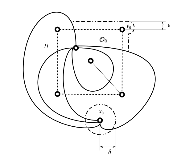
The next two results are central in proving the existence of a downscaling map for a simple, plane, connected graph. The intuitive idea and technique are depicted in Figure 2 (b).

Let $G=(V,E)$ be a connected, simple, plane graph such that no bridges are in the boundary of its outer face. Then, there exists a downscaling map for $G$ . Moreover, this existence can be attained for any chosen level of regularity.

If $G$ has no edges then it must be a single vertex $v$ , thus an open ball centered at $v$ will satisfy the definition of downscaling map. We will henceforth assume that $G$ has at least one edge.

Let $G^{*}$ be the plane dual graph of $G$ drawn with disjoint simple curves as edges. The regions defined by the faces $f^{*}$ of $G^{*}$ are the natural candidate to define a downscaling map of $G$ , however they fail because of two reasons. On one hand, according to Theorem 2 we know that the double dual $G^{**}$ is isomorphic to $G$ . In particular, the outer face of $G^{*}$ must contain a vertex of the plane graph $G$ . On the other hand, given a face $f^{*}$ of the plane dual containing an outer vertex $v$ , it would not necessarily hold that $|\partial f^{*}\cap\partial f^{*}_{0}|>0$ , where $f_{0}^{*}$ is the outer face of $G^{*}$ , as demands the condition (vi) in Definition 10.

We overcome the first deficiency as follows, let $v_{0}$ be the unique vertex in $G$ contained in the outer face $f_{0}^{*}$ of $G^{*}$ and let $C$ be the cycle in $G$ bounding its outer face $f_{0}$ . Clearly $v_{0}$ belongs to $C$ , now let $\epsilon>0$ be such that the tubular $\epsilon$ -region of the induced graph $C-v_{0}$ is completely contained in $(f_{0}^{*})^{c}$ . Define the region

\mathcal{O}_{0}\overset{\mathbf{def}}{=}f_{0}^{*}\cap\bigcup_{x\,\in\,(f_{0})^{c}}B(x,\epsilon).

Since $f_{0}$ is the outer face, it is clear that $f_{0}^{c}$ and $\bigcup_{x\,\in\,(f_{0})^{c}}B(x,\epsilon)$ is simply connected. Therefore $\mathcal{O}_{0}$ is open bounded, simply connected and contains $v_{0}$ . For the second deficiency, let $x_{0}$ be the point representing the outer face $f_{0}$ in the plane dual $G^{*}$ . Now let $\delta>0$ be such that $\cl B(x_{0},\delta)\subset f_{0}$ , then the collection

\{f^{*}-\cl B(x_{0},\delta):f^{*}\;\text{face of}\;G^{*}\}\cup\{\mathcal{O}_{0}-\cl B(x_{0},\delta)\},

constitutes a downscaling map for the graph $G$ .

Finally, since the smooth curves are dense in the plane, it is clear that the boundaries of the elements of this downscaling map can be continuously deformed, to define a new downscaling map with any required level of regularity. ∎

Refer to caption — (a) Starting Graph $G$ .

Let $G$ be a connected, simple, plane graph, let $F$ be the set of bridges in the outer face of $G$ , and $H_{1},...,H_{k}$ be the connected components of the graph defined by removing the edges in $F$ . Let $\tilde{G}$ be the graph whose vertex set is $\{v_{1},...,v_{k}\}$ , where $v_{i}$ is connected to $v_{j}$ if and only if $H_{i}$ is connected to $H_{j}$ by an edge in $F$ . Then, $\tilde{G}$ is a tree.

If $\tilde{G}$ contains a cycle, the removal of one edge in such cycle does not disconnect $\tilde{G}$ . Hence such edge is not a bridge contradicting the definition of $F$ . ∎

Finally, we present the main result of this section.

Let $G=(V,E)$ be a connected, simple, plane graph. Then, there exists a downscaling map with smooth boundaries for $G$ .

First, if $G$ has no cycles then it is a tree and its tubular map constitutes a downscaling map. Hence, from now on we assume that $G$ has at least one cycle.

Let $H_{1},...,H_{k}$ be the components and $\tilde{G}$ be its associated graph as defined in Proposition 6. We will proceed by induction over $k$ . If $k=1$ , then Lemma 5 provides the required downscaling map. If $k>1$ , then renumbering the components if necessary, suppose that $H_{k}$ is such that $v_{k}$ in $\tilde{G}$ is a leaf. Let $\Lambda$ be a downscaling map with smooth boundaries for $H_{k}$ and let $\mathcal{M}$ be its domain. Analogously, let $\Theta$ be a downscaling map with smooth boundaries for the graph such that includes $H_{1},...,H_{k-1}$ together with every bridge connecting these components and let $\mathcal{O}$ be its domain. By deforming their boundaries, it can be additionally assumed that $d(\mathcal{O},\mathcal{M})>0$ , while preserving the smoothness of their boundaries.

Let $v$ and $u$ be the vertices such that $vu$ is the unique bridge connecting $H_{k}$ with some component $H_{i}$ with $1\leq i<k$ . Clearly $v\in H_{k}$ and $u\in H_{i}$ . Denote by $\mathcal{O}_{u}$ and $\mathcal{M}_{v}$ the regions of $\Theta$ and $\Lambda$ containing $u$ and $v$ respectively. Consider the graph $\hat{G}$ consisting of the vertices $u$ , $v$ and the edge $uv$ . Take two points $p$ and $q$ in the interior of the one dimensional manifolds $\partial\mathcal{O}\cap\partial\mathcal{O}_{u}$ and $\partial\mathcal{M}\cap\partial\mathcal{M}_{v}$ respectively. Choose a simple curve $C$ connecting $u$ and $v$ , which intersects $\partial\mathcal{O}$ and $\partial\mathcal{M}$ at the unique points $p$ , $q$ and such such that $d(C,\mathcal{O}^{\prime})$ and $d(C,\mathcal{M}^{\prime})$ are positive; where $\mathcal{O}^{\prime}\overset{\mathbf{def}}{=}\mathcal{O}-\mathcal{O}_{v}$ and $\mathcal{M}^{\prime}\overset{\mathbf{def}}{=}\mathcal{M}-\mathcal{M}_{v}$ . Choose $\epsilon>0$ strictly less than $\mathrm{min}\{d(C,\mathcal{O}^{\prime}),d(C,\mathcal{M}^{\prime})\}$ and such that if $\mathcal{G}$ denotes the $\epsilon$ -map of $\hat{G}$ , then it verifies that $\mathcal{G}\cap\mathcal{O}\subset\mathcal{O}_{u}$ and $\mathcal{G}\cap\mathcal{M}\subset\mathcal{M}_{u}$ . Redefine $\mathcal{O}_{u}$ , $\mathcal{M}_{v}$ in order to include the regions in the tubular $\epsilon$ -map $\mathcal{G}$ , corresponding to $u$ and $v$ respectively. If necessary, deform the boundaries of $\mathcal{O}_{u}$ and $\mathcal{M}_{v}$ to attain the required smoothness and denote the outcome by $O_{u}$ and $M_{v}$ respectively. The collection $\Lambda-\{\mathcal{M}_{v}\}$ , $\Theta-\{\mathcal{O}_{u}\}$ together with $\{O_{u}\}$ and $\{M_{v}\}$ constitutes a downscaling map for $G$ with the required regularity. ∎

In this section we give the geometric setting for the formulation of the problem.

Let $\Omega$ be a connected bounded region with smooth boundary, let $\mathcal{G}=\{K:K\in\mathcal{G}\}$ be a bipartite map and denote by $\mathcal{G}_{1}=\{L:L\in\mathcal{G}_{1}\}$ , $\mathcal{G}_{2}=\{M:M\in\mathcal{G}_{2}\}$ the bipartition, or bi-coloring, of the map.

(i)

For each region $K\in\mathcal{G}$ denote by $\bm{\widehat{\nu}}$ the outer normal vector to its boundary $\partial K$ .

(ii)

For each region $K\in\mathcal{G}$ denote by $\bm{\widehat{n}}:\partial K\rightarrow\bm{\mathbbm{R}}^{N}$ the “normal" vector by

\bm{\widehat{n}}(\vec{x})\overset{\mathbf{def}}{=}\begin{cases}\bm{\widehat{\nu}}(\vec{x})&K\in\mathcal{G}_{1},\\ -\bm{\widehat{\nu}}(\vec{x})&K\in\mathcal{G}_{2}\;\text{and}\;\vec{x}\in\partial K\cap\Omega\,,\\ \bm{\widehat{\nu}}(\vec{x})&K\in\mathcal{G}_{2}\,\text{and}\;\vec{x}\in\partial K\cap\partial\Omega\,.\end{cases}

(8)

(iii)

Define $\displaystyle\Omega_{1}\overset{\mathbf{def}}{=}\bigcup\{L:L\in\mathcal{G}_{1}\}$ , $\displaystyle\Omega_{2}\overset{\mathbf{def}}{=}\bigcup\{M:M\in\mathcal{G}_{2}\}$ .
(iv)

Define $\displaystyle\Gamma\overset{\mathbf{def}}{=}\bigcup\{\partial K:K\in\mathcal{G}\}-\partial\Omega$ .

(v)

Define

\begin{split}\mathcal{E}\overset{\mathbf{def}}{=}\bigcup\{\partial L\cap\partial M:L\in\mathcal{G}_{1},\;M\in\mathcal{G}_{2}\}&=\{\sigma:\sigma\;\text{is the interface of two regions of different type}\}\\ &=\{\sigma:\sigma\;\text{defines an edge in the graph}\;G\;\text{of the map}\;\mathcal{G}\}.\end{split}

(9)

Notice that

(i)

Simple connectedness upon the domain is not required in order to include the tubular map.
(ii)

In agreement with the previous section notice that a bipartite map will always be induced by a bipartite simple graph.

In order to successfully associate a well-posed problem we endow the Problem (1) with boundary conditions (10c), (10f), together with the exchange interface conditions of normal flux balance (10h) and normal stress balance (10h). This gives the following strong problem

	$a\,\mathbf{u}_{1}+\bm{\nabla}p_{1}+\mathbf{g}=0\,,$		(10a)
	$\bm{\nabla}\cdot\mathbf{u}_{1}=F\,\quad\mathrm{in}\;\Omega_{1}\,.$		(10b)
	$p_{1}=0\quad\mathrm{on}\;\partial\Omega_{1}\cap\partial\Omega\,.$		(10c)
	$a\,\mathbf{u}_{2}+\bm{\nabla}p_{2}+\mathbf{g}=0\,,$		(10d)
	$\bm{\nabla}\cdot\mathbf{u}_{2}=F\,\quad\mathrm{in}\;\Omega_{2}.$		(10e)
	$\mathbf{u}_{2}\cdot\bm{\widehat{n}}=0\quad\mathrm{on}\;\partial\Omega_{2}\cap\partial\Omega,$		(10f)
	$\mathbf{u}_{1}\cdot\bm{\widehat{n}}-\mathbf{u}_{2}\cdot\bm{\widehat{n}}=\beta\,p_{2}+f_{\bm{\hat{n}}}\,,$		(10g)
	$p_{2}-p_{1}=f_{\Sigma}\,\quad\mathrm{on}\;\Gamma\,.$		(10h)

It will be assumed that the storage exchange and the friction coefficients, $\beta:\Gamma\rightarrow[0,\infty)$ , $a:\Omega\rightarrow(0,\infty)$ respectively, verify that $\beta\in L^{\infty}(\Gamma)$ , $\|\beta\,\bm{\mathbbm{1}}_{\Gamma}\|_{L^{1}(\Gamma)}>0$ and $a\in L^{\infty}(\Omega)$ , $\|\frac{1}{a}\|_{L^{\infty}(\Omega)}>0$ .

In order to introduce the modeling spaces used in the formulation we first notice that $\{L:L\in\mathcal{G}_{1}\}$ and $\{M:M\in\mathcal{G}_{2}\}$ are the simply connected components of $\Omega_{1}$ and $\Omega_{2}$ respectively. Then,

\displaystyle\mathbf{H_{div}}(\Omega_{1})=\bigoplus_{L\,\in\,\mathcal{G}_{1}}\mathbf{H_{div}}(L),

\displaystyle H^{1}(\Omega_{2})=\bigoplus_{M\,\in\,\mathcal{G}_{2}}H^{1}(M).

The following space is introduced in order to couple adequately, the action of the pressures traces in the variational formulation

\begin{split}E(\Omega_{2})\overset{\mathbf{def}}{=}&\big\{q\in H^{1}(\Omega_{2}):q\bm{\mathbbm{1}}_{\partial M\cap\partial L}\in H^{1/2}(\partial L)\;\text{for all }\,(L,M)\in\mathcal{G}_{1}\times\mathcal{G}_{2}\big\}\\ =&\big\{q\in H^{1}(\Omega_{2}):q\bm{\mathbbm{1}}_{\Gamma}\in H^{1/2}(\Gamma)\}.\end{split}

(11)

We endow $E(\Omega_{2})$ with the $H^{1}(\Omega_{2})$ inner product. It is direct to see that $E(\Omega_{2})$ is a closed subspace of $H^{1}(\Omega_{2})$ and consequently a Hilbert space. Now define

\mathbf{V}(\Omega_{2})\overset{\mathbf{def}}{=}\big\{\mathbf{v}\in\mathbf{L}^{\!2}(\Omega_{2}):\mathbf{v}_{2}=\bm{\nabla}q_{2}\;\text{for some}\;q_{2}\in E(\Omega_{2})\big\}=\bm{\nabla}(E(\Omega_{2})),

(12)

endowed with the $\mathbf{L}^{2}(\Omega_{2})$ inner product. Next we show a necessary result.

Let $E(\Omega_{2})$ and $\mathbf{V}(\Omega_{2})$ be as defined in (11), (12) respectively, and define

E_{0}(\Omega_{2})\overset{\mathbf{def}}{=}\Big\{q_{2}\in E(\Omega_{2}):\int_{\Omega_{2}}q_{2}=0\Big\}.

(13)

Then,

(i)

There exists a constant $C>0$ depending only on the domain $\Omega_{2}$ such that

$\displaystyle\|r_{2}\|_{1,\Omega_{2}}\leq C\|\bm{\nabla}r_{2}\|_{0,\Omega_{2}},$ $\displaystyle\text{for all }\;r_{2}\in H\,.$ (14)
(ii)

The space $\mathbf{V}(\Omega_{2})$ is Hilbert.

(i)

Clearly $E_{0}(\Omega_{2})$ is closed and because of the matching property of traces for elements of $E(\Omega_{2})$ the application $r_{2}\mapsto\|\bm{\nabla}r_{2}\|_{0,\Omega_{2}}$ is norm in $E_{0}(\Omega_{2})$ . Due to the Rellich-Kondrachov Theorem this norm is equivalent to the standard one in $E_{0}(\Omega_{2})$ i.e., there exists $C>0$ depending only on the domain $\Omega_{2}$ satisfying the statement (14).
(ii)

Clearly, it is only necessary to check that $\mathbf{V}(\Omega_{2})$ is complete. Let $\{\mathbf{v}_{2}^{n}:n\in\bm{\mathbbm{N}}\}$ be a Cauchy sequence in $\mathbf{V}(\Omega_{2})$ , then there exists a sequence $\{p_{2}^{n}:n\in\bm{\mathbbm{N}}\}$ in $E(\Omega_{2})$ such that $\bm{\nabla}q_{2}^{n}=\mathbf{v}_{2}^{n}$ , then, the function $r_{2}^{n}\overset{\mathbf{def}}{=}q_{2}^{n}-\frac{1}{|\Omega_{2}|}\int_{\Omega_{2}}q_{2}^{n}$ belongs to $E_{0}(\Omega_{2})$ and $\bm{\nabla}r_{2}=\mathbf{v}_{2}$ . Due to the previous part it follows that the sequence $\{r_{2}^{n}:n\in\bm{\mathbbm{N}}\}\subseteq E_{0}(\Omega_{2})$ is Cauchy, consequently it converges to an element $r_{2}\in E_{0}(\Omega_{2})\subseteq E(\Omega_{2})$ . Finally, since the gradient map $\bm{\nabla}$ from $E(\Omega_{2})$ onto $\mathbf{V}(\Omega_{2})$ is continuous, the result follows. ∎

Now we are ready to introduce the functional setting of the problem, we have

	$\mathbf{X}\overset{\mathbf{def}}{=}\mathbf{H_{div}}(\Omega_{1})\times E(\Omega_{2}),$	(15a)
	$\mathbf{Y}\overset{\mathbf{def}}{=}\mathbf{V}(\Omega_{2})\times L^{2}(\Omega_{1}).$	(15b)
Endowed with their natural inner product and norms
	$\big\\|[\mathbf{v}_{1},q_{2}]\big\\|_{\mathbf{X}}\overset{\mathbf{def}}{=}\big\{\\|\mathbf{v}_{1}\\|_{\mathbf{H_{div}}(\Omega_{1})}^{2}+\\|q_{2}\\|_{H^{1}(\Omega_{2})}^{2}\big\}^{\tfrac{1}{2}},$	(15c)
	$\big\\|[\mathbf{v}_{2},q_{1}]\big\\|_{\mathbf{Y}}\overset{\mathbf{def}}{=}\big\{\\|\mathbf{v}_{2}\\|_{\mathbf{L}^{2}(\Omega_{2})}^{2}+\\|q_{1}\\|_{L^{2}(\Omega_{1})}^{2}\big\}^{\tfrac{1}{2}}.$	(15d)

(i)

Notice that the definition of spaces gathers the functions of high regularity in $\mathbf{X}$ and the functions of low regularity in $\mathbf{Y}$ . This choice is made on one hand to satisfy the hypotheses of Theorem 4 and, on the other hand, to preserve the remarkable aspect that the underlying modeling spaces $\mathbf{X}$ and $\mathbf{Y}$ are free of coupling conditions. This approach will lead to a version of mixed formulation different from the one presented in [10] and [14], which shares the coupling-free spaces feature.

In order to avoid heavy notation, in the sequel we adopt the following conventions

(ii)

Let $\Delta$ be an open bounded set, $\mathbf{v}\in\mathbf{H_{div}}(\Delta)$ and $q\in H^{1}(\Delta)$ , then we denote

\int_{\partial\Delta}\big(\mathbf{v}\cdot\bm{\widehat{n}}\big)\,q\;dS\overset{\mathbf{def}}{=}\big\langle\mathbf{v}\cdot\bm{\widehat{n}},q\big\rangle_{H^{-1/2}(\partial\Delta),H^{-1/2}(\partial\Delta)}.

(16)

(iii)

Since $\Gamma=\bigcup_{\sigma\,\in\,{\mathcal{E}}}\sigma$ we denote

\int_{\Gamma}\left(\mathbf{v}_{1}\cdot\bm{\widehat{n}}\right)q_{2}\,dS\overset{\mathbf{def}}{=}\sum_{\sigma\,\in\,\mathcal{E}}\int_{\sigma}\left(\mathbf{v}_{1}\cdot\bm{\widehat{n}}\right)q_{2}\,dS.

(17)

In this section we present a particular mixed-mixed formulation for the problem (10).

	$\text{Find}\;\big([\mathbf{u}_{1},p_{2}],[\mathbf{u}_{2},p_{1}]\big)\in\mathbf{X}\times\mathbf{Y}:\quad\int_{\Omega_{1}}a\,\mathbf{u}_{1}\cdot\mathbf{v}_{1}+\int_{\Gamma}\beta\,p_{2}\,q_{2}\,dS-\int_{\,\Gamma}\left(\mathbf{u}_{1}\cdot\bm{\widehat{n}}\right)q_{2}\,dS+\int_{\,\Gamma}p_{2}\left(\mathbf{v}_{1}\cdot\bm{\widehat{n}}\right)\,dS\\ -\int_{\Omega_{1}}p_{1}\,\bm{\nabla}\cdot\mathbf{v}_{1}\,-\int_{\Omega_{2}}\mathbf{u}_{2}\cdot\bm{\nabla}q_{2}\,=\int_{\Omega_{2}}F\,q_{2}-\int_{\Omega_{1}}\mathbf{g}\cdot\mathbf{v}_{1}+\int_{\Gamma}f_{\Sigma}\,(\mathbf{v}_{1}\cdot\bm{\widehat{n}})\,dS-\int_{\Gamma}f_{\bm{\hat{n}}}\,q_{2}\,dS,$		(18a)
	$\int_{\Omega_{1}}\bm{\nabla}\cdot\mathbf{u}_{1}\,q_{1}+\int_{\Omega_{2}}\bm{\nabla}p_{2}\cdot\mathbf{v}_{2}+\int_{\Omega_{2}}a\,\mathbf{u}_{2}\cdot\mathbf{v}_{2}\,\\ =\int_{\Omega_{1}}F\,q_{1}-\int_{\Omega_{2}}\mathbf{g}\cdot\mathbf{v}_{2}\quad\text{ for all }\big([\mathbf{v}_{1},q_{2}],[\mathbf{v}_{2},q_{1}]\big)\in\mathbf{X}\times\mathbf{Y}.$		(18b)

Define the operators ${\mathcal{A}}:\mathbf{X}\rightarrow\mathbf{X}^{\prime}$ , ${\mathcal{B}}:\mathbf{X}\rightarrow\mathbf{Y}\,^{\prime}$ and ${\mathcal{C}}:\mathbf{Y}\rightarrow\mathbf{Y}\,^{\prime}$ by

	${\mathcal{A}}[\mathbf{v}_{1},q_{2}],\big([\mathbf{w}_{1},r_{2}]\big)\overset{\mathbf{def}}{=}\int_{\Omega_{1}}a\,\mathbf{v}_{1}\cdot\mathbf{w}_{1}+\int_{\Gamma}\beta\,q_{2}\,r_{2}\,dS\\ -\int_{\,\Gamma}\left(\mathbf{v}_{1}\cdot\bm{\widehat{n}}\right)r_{2}\,dS+\int_{\,\Gamma}q_{2}\left(\mathbf{w}_{1}\cdot\bm{\widehat{n}}\right)\,dS,$		(19a)
	${\mathcal{B}}[\mathbf{v}_{1},\,q_{2}],\big([\mathbf{w}_{2},\,r_{1}]\big)\overset{\mathbf{def}}{=}\int_{\Omega_{1}}\bm{\nabla}\cdot\mathbf{v}_{1}\,r_{1}+\int_{\Omega_{2}}\bm{\nabla}q_{2}\cdot\mathbf{w}_{2},\,$		(19b)
	${\mathcal{C}}[\mathbf{v}_{2},\,q_{1}]\big([\mathbf{w}_{2},\,r_{1}]\big)\overset{\mathbf{def}}{=}\int_{\Omega_{2}}a\,\mathbf{v}_{2}\cdot\mathbf{w}_{2}.$		(19c)

Thus, the Problem (18) is equivalent to

\begin{split}\text{Find a pair}\;\big([\mathbf{u}_{2},\,p_{1}],[\mathbf{u}_{1},\,p_{2}]\big)\in\mathbf{X}\times\mathbf{Y}:\quad{\mathcal{A}}[\mathbf{u}_{2},\,p_{1}]+{\mathcal{B}}^{\prime}[\mathbf{u}_{1},\,p_{2}]=F_{1}\quad\text{in}\;\mathbf{X}^{\prime},\\ -{\mathcal{B}}[\mathbf{u}_{2},\,p_{1}]+{\mathcal{C}}[\mathbf{u}_{1},\,p_{2}]=F_{2}\quad\text{in}\;\mathbf{Y}^{\prime}.\end{split}

(20)

Where $F_{1}\in\mathbf{X}^{\prime}$ and $F_{2}\in\mathbf{Y}^{\prime}$ are the functionals defined by the right hand side of (18a) and (18b) respectively.

The operator ${\mathcal{B}}:\mathbf{X}\rightarrow\mathbf{Y}^{\prime}$ defined in equation (19b) is continuous and satisfies the $\inf-\sup$ condition i.e., there exists a constant $C>0$ depending only on the map $\mathcal{G}$ such that for every $[\mathbf{w}_{2},r_{1}]\in\mathbf{Y}$ there exists $[\mathbf{v}_{1},q_{2}]\in\mathbf{X}$ satisfying

{\mathcal{B}}\,[\mathbf{v}_{1},q_{2}]([\mathbf{w}_{2},r_{1}])\geq C\,\big\|[\mathbf{v}_{1},q_{2}]\big\|_{\mathbf{X}}\big\|[\mathbf{w}_{2},r_{1}]\big\|_{\mathbf{Y}}\,.

(21)

Moreover, the constant $C>0$ is independent from $[\mathbf{w}_{2},r_{1}]$ .

It is direct to see that the operator ${\mathcal{B}}$ is continuous. Now fix $[\mathbf{w}_{2},r_{1}]\;\in\mathbf{Y}$ , for each polygon $L\in\mathcal{G}_{1}$ let $\xi_{L}\in H_{0}^{1}(L)$ be the unique solution of the local homogeneous Dirichlet problem

\displaystyle-\bm{\nabla}\cdot\bm{\nabla}\xi_{L}=r_{1}\,\bm{\mathbbm{1}}_{L}\quad\text{in}\;L,

\displaystyle\xi_{L}=0\quad\text{on}\;\partial L.

(22)

Taking $\mathbf{v}_{L}\overset{\mathbf{def}}{=}\bm{\nabla}\xi_{L}$ due to Poincaré inequality we observe that $\|\mathbf{v}_{L}\|_{\mathbf{H_{div}}(L)}\leq C_{L}\,\|r_{1}\bm{\mathbbm{1}}_{L}\|_{0,L}$ where $C_{L}$ depends only on the diameter of the simply connected region $L$ . Therefore, the function $\mathbf{v}_{1}\overset{\mathbf{def}}{=}\sum_{L\,\in\,\mathcal{G}_{1}}\mathbf{v}_{L}\,\bm{\mathbbm{1}}_{L}$ clearly belongs to $\mathbf{H_{div}}(\Omega_{1})$ and $\|\mathbf{v}_{1}\|_{\mathbf{H_{div}}(\Omega_{1})}\leq\big(\max_{L\,\in\,\mathcal{G}_{1}}C_{L}\big)\,\|r_{1}\|_{0,\Omega_{1}}$ .

Let $\mathbf{w}_{2}\in\mathbf{V}(\Omega_{2})$ , by definition there must exist $\eta\in E(\Omega_{2})$ such that $\bm{\nabla}\eta=\mathbf{v}_{2}$ . Then, $q_{2}\overset{\mathbf{def}}{=}\eta-\frac{1}{|\Omega_{2}|}\int_{\Omega_{2}}\eta$ belongs to the space $E_{0}(\Omega_{2})$ (defined in (13)), it satisfies that $\bm{\nabla}r_{2}=\mathbf{w}_{2}$ and due to the Inequality (14), it holds that $\|q_{2}\|_{1,\Omega_{2}}\leq C\,\|\mathbf{v}_{2}\|_{0,\Omega_{2}}$ with $C>0$ depending only on the domain $\Omega_{2}$ .

Hence, the pair $[\mathbf{v}_{1},q_{2}]$ belongs to $\mathbf{X}$ and $C\,\big\|[\mathbf{v}_{1},q_{2}]\big\|_{\mathbf{X}}\leq\big\|[\mathbf{w}_{2},r_{1}]\big\|_{\mathbf{Y}}$ for an adequate constant $C>0$ independent from $[\mathbf{w}_{2},r_{1}]$ . Moreover,

{\mathcal{B}}[\mathbf{v}_{1},q_{2}]\big([\mathbf{w}_{2},r_{1}]\big)=\big\|[\mathbf{w}_{2},r_{1}]\big\|_{\mathbf{Y}}^{2}\geq C\,\big\|[\mathbf{v}_{1},q_{2}]\big\|_{\mathbf{X}}\,\big\|[\mathbf{w}_{2},r_{1}]\big\|_{\mathbf{Y}}\,.

The inequality above yields the inf-sup condition (21). ∎

The operator ${\mathcal{A}}:\mathbf{X}\rightarrow\mathbf{X}\,^{\prime}$ defined by (19a) is $\mathbf{X}$ -coercive on $\mathbf{X}\cap\ker({\mathcal{B}})$ i.e.,

{\mathcal{A}}[\mathbf{v}_{1},q_{2}]\big([\mathbf{v}_{1},q_{2}]\big)\geq C\big\|[\mathbf{v}_{1},q_{2}]\big\|_{\mathbf{X}}^{2}\,,\quad\text{for all}\;[\mathbf{v}_{1},q_{2}]\in\mathbf{X}\cap\ker({\mathcal{B}}).

(23)

Where $C>0$ is an adequate constant depending only on the map $\mathcal{G}$ and the storage coefficient $\beta$ .

The continuity of the operator ${\mathcal{A}}$ follows applying the Cauchy-Schwartz inequality on each of its summands and noticing that the boundary terms involved can be controlled by the norm $\|\cdot\|_{\mathbf{X}}$ . For the coerciveness of the operator, let $[\mathbf{v}_{1},q_{2}]\in\mathbf{X}\cap\ker({\mathcal{B}})$ then

{\mathcal{B}}[\mathbf{v}_{1},q_{2}]\big([\mathbf{w}_{2},r_{1}]\big)=0\quad\text{for all}\;[\mathbf{w}_{2},r_{1}]\in\mathbf{Y}.

(24)

In particular, testing (24) with $[\bm{0},r_{1}]\in\mathbf{Y}$ we conclude that $\bm{\nabla}\cdot\mathbf{v}_{1}=0$ since $r_{1}$ is an arbitrary element in $L^{2}(\Omega_{1})$ . On the other hand, clearly $\bm{\nabla}q_{2}\in\mathbf{V}(\Omega_{2})$ and the pair $[\bm{\nabla}q_{2},0]\in\mathbf{Y}$ is eligible for testing (24). The test yields $\bm{\nabla}q_{2}=\bm{0}$ i.e., $q_{2}$ is constant inside $\Omega_{2}$ . Hence

\int_{\Gamma}\beta\,q_{2}^{2}=\frac{\|\beta\,\bm{\mathbbm{1}}_{\partial\Gamma}\|_{L^{1}(\Gamma)}}{|\Omega_{2}|}\,\|q_{2}\|_{0,\Omega_{2}}^{2}=\frac{\|\beta\,\bm{\mathbbm{1}}_{\Gamma}\|_{L^{1}(\Gamma)}}{|\Omega_{2}|}\,\|q_{2}\bm{\mathbbm{1}}_{\Omega_{2}}\|_{1,\Omega_{2}}^{2}.

Using the previous observations we get that

\begin{split}{\mathcal{A}}[\mathbf{v}_{1},q_{2}]\big([\mathbf{v}_{1},q_{2}]\big)&=\int_{\Omega_{1}}a\mathbf{v}_{1}\cdot\mathbf{v}_{1}+\int_{\Gamma}\beta\,q_{2}^{2}\,dS\\ &\geq\Big\|\frac{1}{a}\Big\|^{-1}_{L^{\infty}(\Omega)}\|\mathbf{v}_{1}\|^{2}_{\mathbf{H_{div}}(\Omega_{1})}+\frac{\|\beta\,\bm{\mathbbm{1}}_{\Gamma}\|_{L^{1}(\Gamma)}}{|\Omega_{2}|}\,\|q_{2}\|_{1,\Omega_{2}}^{2}\\ &\geq C\,\big\|[\mathbf{v}_{1},q_{2}]\big\|_{\mathbf{X}}^{2}\,,\end{split}

where $C=\min\big\{\|\frac{1}{a}\|^{-1}_{L^{\infty}(\Omega)},\,|\Omega_{2}|^{-1}\,\|\beta\,\bm{\mathbbm{1}}_{\Gamma}\|_{L^{1}(\Gamma)}\,\big\}$ . This completes the proof. ∎

The Problem (20) is well-posed and there exist a constant $C>0$ depending only on the map $\mathcal{G}$ such that

\big\|[\mathbf{u}_{2},\,p_{1}]\big\|_{\mathbf{X}}+\big\|[\mathbf{u}_{1},\,p_{2}]\big\|_{\mathbf{Y}}\leq C\,(\|F_{1}\|_{\mathbf{X}^{\prime}}+\|F_{2}\|_{\mathbf{Y}^{\prime}}).

The proof is a direct application of Theorem 4 as all the required hypotheses are satisfied. ∎

We begin this section with the strong problem that is modeled by the weak variational formulation (18). The process shows mild restrictions on the forcing terms which are characterized below.

The solution of the weak variational problem (18) is a strong solution of the problem (10) with the forcing gravitation term $\mathbf{g}$ in the equation (10a) replaced by $P\mathbf{g}$ , which denotes its orthogonal projection onto the space $\mathbf{V}(\Omega_{2})$ . In particular if $\mathbf{g}\bm{\mathbbm{1}}_{\Omega_{2}}\in\mathbf{V}(\Omega_{2})$ the weak solution is exactly the strong solution.

First we focus on recovering the constitutive and conservative equations (10a), (10b), (10e) and (10d), on the domains $\Omega_{1}$ and $\Omega_{2}$ respectively.

Choose $[\bm{0},q_{1}]\in\mathbf{Y}$ and test equation (18b) to get $\int_{\Omega_{1}}\bm{\nabla}\cdot\mathbf{u}_{1}\,q_{1}=\int_{\Omega_{1}}F\,q_{1}$ , for all $q_{1}\in L^{2}(\Omega_{1})$ . This yields the strong conservation equation (10b). Next choose $[\mathbf{v}_{2},0]\in\mathbf{Y}$ and test equation (18b) to get $\int_{\Omega_{2}}(\bm{\nabla}p_{2}+a\,\mathbf{u}_{2})\cdot\mathbf{v}_{2}=-\int_{\Omega_{2}}\mathbf{g}\cdot\mathbf{v}_{2}$ . Clearly $\bm{\nabla}p_{2}+a\,\mathbf{u}_{2}\in\mathbf{V}(\Omega_{2})$ and the previous equality holds for all $\mathbf{v}_{2}\in\mathbf{V}(\Omega_{2})$ . From here it follows that $\bm{\nabla}p_{2}+a\,\mathbf{u}_{2}=-P\mathbf{g}$ , where $P\mathbf{g}$ is the orthogonal projection of $\mathbf{g}$ onto $\mathbf{V}(\Omega_{2})$ . This gives the constitutive Darcy equation (10d) with the forcing term $\mathbf{g}$ replaced by its projection $P\mathbf{g}$ . Now let $\Phi\in[C_{0}^{\infty}(\Omega_{1})]^{N}$ then, testing equation (18a) with $[\Phi,0]\in\mathbf{X}$ we get

\int_{\Omega_{1}}a\,\mathbf{u}_{1}\cdot\Phi-\int_{\Omega_{1}}p_{1}\,\bm{\nabla}\cdot\Phi\,=-\int_{\Omega_{1}}\mathbf{g}\cdot\Phi.

The above holds for all $\Phi\in[C_{0}^{\infty}(\Omega_{1})]^{N}$ then, the equation (10a) follows in the $\mathbf{H}^{-1}(\Omega_{1})$ -sense. Moreover, recalling that $\mathbf{u}_{1},\mathbf{g}\in\mathbf{L}^{2}(\Omega_{1})$ , the strong constitutive Darcy equation (10a) also holds in the $\mathbf{L}^{2}(\Omega_{1})$ -sense. Now let $\varphi\in C_{0}^{\infty}(\Omega_{1})$ and test equation (18a) with $[\bm{0},\varphi]\in\mathbf{X}$ to get $-\int_{\Omega_{2}}\mathbf{u}_{2}\cdot\bm{\nabla}\varphi=\int_{\Omega_{2}}F\,\varphi$ . Since this holds for all smooth functions the strong conservative equation (10e) follows.

Next we focus on the boundary and the interface conditions. Take $\mathbf{v}_{1}\in\mathbf{H_{div}}(\Omega_{1})$ , test (10a) with $[\mathbf{v}_{1},0]\in\mathbf{X}$ , integrate by parts and get

\int_{\Omega_{1}}a\,\mathbf{u}_{1}\cdot\mathbf{v}_{1}+\int_{\,\Gamma}p_{2}\big(\mathbf{v}_{1}\cdot\bm{\widehat{n}}\big)\,dS\\ +\int_{\Omega_{1}}\bm{\nabla}p_{1}\cdot\mathbf{v}_{1}-\int_{\partial\Omega_{1}}p_{1}\,\big(\mathbf{v}_{1}\cdot\bm{\widehat{\nu}}\big)\,dS\,=-\int_{\Omega_{1}}\mathbf{g}\cdot\mathbf{v}_{1}+\int_{\Gamma}f_{\Sigma}\,\big(\mathbf{v}_{1}\cdot\bm{\widehat{n}}\big)\,dS.

We split the boundary term on $\partial\Omega_{1}$ in two pieces, the interfaces network $\Gamma$ and the outer part $\partial\Omega_{1}-\Gamma=\partial\Omega_{1}\cap\partial\Omega$ and replace $\bm{\widehat{\nu}}$ with $\bm{\widehat{n}}$ using the relationship given in Definition 11, equation (8). Additionally, recalling that the identity (10a) is satisfied, the expression above writes as

\int_{\,\Gamma}p_{2}\big(\mathbf{v}_{1}\cdot\bm{\widehat{n}}\big)\,dS\\ -\int_{\Gamma}p_{1}\,\big(\mathbf{v}_{1}\cdot\bm{\widehat{\nu}}\big)\,dS-\int_{\partial\Omega_{1}\cap\partial\Omega}p_{1}\,\big(\mathbf{v}_{1}\cdot\bm{\widehat{\nu}}\big)\,dS\,=\int_{\Gamma}f_{\Sigma}\,\big(\mathbf{v}_{1}\cdot\bm{\widehat{n}}\big)\,dS.

Since the above holds for all $\mathbf{v}_{1}\in\mathbf{H_{div}}(\Omega_{1})$ and the map $\mathbf{v}_{1}\mapsto\mathbf{v}_{1}\cdot\bm{\widehat{n}}$ from $\mathbf{H_{div}}(\Omega_{1})$ onto $H^{-1/2}(\partial\Omega_{1})$ is surjective, the normal stress balance condition across the interfaces (10h) and the drained Dirichlet boundary condition (10c) follow in the sense of $H^{1/2}(\Gamma)$ and $H^{1/2}(\partial\Omega_{1}\cap\partial\Omega)$ respectively. Finally, taking $q_{2}\in H^{1}(\Omega_{2})$ , testing (10a) with $[\bm{0},q_{2}]\in\mathbf{X}$ and integrating by parts we get

\int_{\Gamma}\beta\,p_{2}\,q_{2}\,dS-\int_{\,\Gamma}\big(\mathbf{u}_{1}\cdot\bm{\widehat{n}}\big)q_{2}\,dS\\ +\int_{\Omega_{2}}\bm{\nabla}\cdot\mathbf{u}_{2}\,q_{2}-\int_{\partial\Omega_{2}}\big(\mathbf{u}_{2}\cdot\bm{\widehat{\nu}}\big)q_{2}\,dS=\int_{\Omega_{2}}F\,q_{2}-\int_{\Gamma}f_{\bm{\hat{n}}}\,q_{2}\,dS.

(25)

Again, we split the boundary term on $\partial\Omega_{2}$ in two pieces, the interfaces network $\Gamma$ and the outer part $\partial\Omega_{2}-\Gamma=\partial\Omega_{2}\cap\partial\Omega$ ; then replace $\bm{\widehat{\nu}}$ with $\bm{\widehat{n}}$ using the relationship given in Definition 11, equation (8). Since the identity (10e) is satisfied, the expression above reduces to

\int_{\Gamma}\beta\,p_{2}\,q_{2}\,dS-\int_{\,\Gamma}\left(\mathbf{u}_{1}\cdot\bm{\widehat{n}}\right)q_{2}\,dS\\ +\int_{\Gamma}(\mathbf{u}_{2}\cdot\bm{\widehat{n}})q_{2}\,dS-\int_{\partial\Omega_{2}\cap\Omega}(\mathbf{u}_{2}\cdot\bm{\widehat{n}})q_{2}\,dS=-\int_{\Gamma}f_{\bm{\hat{n}}}\,q_{2}\,dS.

(26)

Observing that the above holds for all $q_{2}\in E(\Omega_{2})$ , it follows that the normal flux balance condition across the interfaces (10g) and the null normal flux boundary condition (10f) hold, in the sense of $H^{-1/2}(\Gamma)$ and $H^{-1/2}(\partial\Omega_{2}\cap\partial\Omega)$ respectively. This completes the proof. ∎

Finally in order to identify which forcing terms can be modeled using this formulation, this section closes characterizing the orthogonal projection onto the spaces $\mathbf{V}(\Omega_{2})$ and $\mathbf{V}^{\perp}(\Omega_{2})$ .

Let $\mathbf{v}\in\mathbf{L}^{2}(\Omega_{2})$ . Let $\xi\in H_{0}^{1}(\Omega)\subseteq E(\Omega_{2})$ and $\eta\in E_{0}(\Omega_{2})$ be the unique solutions of the respective Dirichlet and Neumann problems

Then, $\mathbf{v}-\bm{\nabla}\xi-\bm{\nabla}\eta$ is the projection of $\mathbf{v}$ onto $\mathbf{V}^{\perp}(\Omega_{2})$ and $\bm{\nabla}\xi+\bm{\nabla}\eta$ is the projection of $\mathbf{v}$ onto $\mathbf{V}(\Omega_{2})$ .

First recall that since $C_{0}^{\infty}(\Omega_{2})\subseteq E(\Omega_{2})$ then

\mathbf{V}^{\perp}(\Omega)=\big\{\mathbf{v}\in\mathbf{L}^{2}(\Omega_{2}):\bm{\nabla}\cdot\mathbf{v}=0,\,\text{in }\,\Omega_{2}\;\text{and }\,\mathbf{v}\cdot\bm{\widehat{n}}=0\,,\;\text{on }\,\partial\Omega_{2}\big\},

i.e. $\mathbf{V}^{\perp}(\Omega_{2})\subseteq\mathbf{H_{div}}(\Omega_{2})$ . Next, observe that since $\xi\in H_{0}^{1}(\Omega_{2})$ then $\bm{\nabla}\xi\in\mathbf{L}^{2}(\Omega_{2})$ , and because it is a solution to problem (27a) it follows that $\bm{\nabla}\cdot(\mathbf{v}-\bm{\nabla}\xi)=0$ i.e., $\mathbf{v}-\bm{\nabla}\xi\in\mathbf{H_{div}}(\Omega_{2})$ . Moreover, for any $q\in H^{1}(\Omega_{2})$ it holds that

\big\langle(\mathbf{v}-\bm{\nabla}\xi)\cdot\bm{\widehat{n}},q\big\rangle_{H^{-1/2}(\partial\Omega_{2}),H^{-1/2}(\partial\Omega_{2})}=\int_{\Omega_{2}}(\mathbf{v}-\bm{\nabla}\xi)\cdot\bm{\nabla}q.

In particular, if $q=1$ then $\big\langle(\mathbf{v}-\bm{\nabla}\xi)\cdot\bm{\widehat{n}},1\big\rangle_{H^{-1/2}(\partial\Omega_{2}),H^{-1/2}(\partial\Omega_{2})}=0$ i.e., the data for the Neumann problem (27b) satisfy the compatibility condition and the problem has a unique solution $\eta$ in $E_{0}(\Omega_{2})$ . Now, it is clear that $\mathbf{v}-\bm{\nabla}\xi-\bm{\nabla}\eta\in\mathbf{H}(\Omega_{2})$ and since $\mathbf{v}-(\mathbf{v}-\bm{\nabla}\xi-\bm{\nabla}\eta)=\bm{\nabla}\xi+\bm{\nabla}\eta$ is orthogonal to $\mathbf{H}(\Omega_{2})$ , the result follows due to the characterization of orthogonal projections in Hilbert spaces. ∎

The present work yields several as summarized below.

(i)

The study of communication in complex networks, as stated in [1, 4], can be perplexing due to the large number of nodes and links. One of the greatest achievements of this article is to provide a relatively simple upscaled description to an otherwise very complicated study. This result gives the grounds to use well-studied numerical methods such as Finite Elements on Complex Network Theory.
(ii)

The function $a(\cdot)$ presented in the strong form (10a), (10a), can be used as a scaling tool. If the volume of a region does not correctly reflect the impact of the universe it represents within the multiverse then, $a(\cdot)$ can be scaled in that region to counterbalance this deficiency and weigh each region of the map accordingly.
(iii)

The interface conditions (10g) and (10h), allow discontinuities along paths in the domain. This permits the modeling of sinks and/or sources on different manifolds along the region of interest.
(iv)

The method for PDE analysis on graphs presented in this article and the previous achievements in the literature are dual concepts. The preexisting results rely on complex definitions for the operators of the PDE and simple definitions for the domain. This work introduces simple definitions for the operators of the PDE and very restrictive definitions for the graph. As many results in mathematics have shown, complementing dual concepts and a wise interplay between them, are the key for a very strong theory. The result presented proves that this method for analyzing PDE on graphs is the gateway for significantly deeper understanding in the field.
(v)

In the articles [10] and [14], a similar mixed variational formulation is introduced in order to model the saturated fluid flow within a fractured porous medium. This result is an alternative version, allowing to treat fractures with substantially more general geometry. Additionally, the mixed variational formulation presented here is, to the authors’ best knowledge, unprecedented in the specialized literature of PDE analysis.

For the limitations of the method we point out the following ones.

(i)

There are two particularly important cases of discretization for 3-D polygonal domains in a bipartite fashion, using tetrahedra as discussed in [15], or using in cubes. For both cases, it is not difficult to prove that a subdivision of the graph $K_{3,3}$ is contained in most of the graphs, defined by the “tetrahedral grids" or the “cubic grids", associated to a given domain. Therefore, most of the time, the associated graph is nonplanar and bipartite. Although in these scenarios the domain for the PDE setting is already defined, the nonplanar structure of their natural associated graphs suggests that the analysis for bipartite, nonplanar graphs is an important issue still to be addressed.
(ii)

The variational formulation is dependent upon the domain chosen for the graph at hand. Thus, the construction of the domain that suits the application best will depend on the context. In this article we have suggested two possible choices, namely the tubular and downscaling maps.

Finally, for further work we highlight the following aspects.

(i)

The method of analyzing highly clustered complex networks presented here is based upon the assumption that, approximating the behavior of a large number of particles with an open set, introduces an acceptable error when they are highly clustered. In order to understand the extent of this claim, further work about the error introduced by this approximation is of central importance. Notice that the quality of the approximation may very well depend on the nature of the quantities one is considering, which will impact in the PDE model. This aspect will be explored in future work.
(ii)

The Darcy Flow Model is a more general case of the Poisson equation whose unique differential operator is the Laplacian. Discrete versions of the Laplacian Operator for graphs are presented in [5, 6, 16]. A natural conjecture is that the discrete Laplacian operator will approximate the continuous version if the number of nodes is very large. This conjecture will be addressed in future work, because it may provide the foundation to justify the claim that, jumping from discrete to continuous is a reasonable estimate for the global behavior when the number of nodes is large.
(iii)

The formulation introduced divides the domain in two types of regions, namely $\Omega_{1}$ and $\Omega_{2}$ which is the reason why the main setting of the problem had to be bipartite. Since every plane map is four coloreable it remains for future work to find a formulation addressing up to four types of regions.

The authors wish to acknowledge Universidad Nacional de Colombia, Sede Medellín for its support in this work through the project HERMES 27798. They also wish to thank Tomás Mejía for his constructive criticism and insightful suggestions in this work.

[1] E. Estrada, The Structure of Complex Networks, Theory and Applications, Oxford University Press, New York, 2012.
[2] L. Orsenigo, Clusters and clustering in biotechnology: Stylised facts, issues and theories. In: Braunerhjelm, Pontus and Feldman, Maryann P. eds. Cluster Genesis. Oxford University Press, pp 195–218, 2006.
[3] M. O. Jackson, Social and Economic Networks, Princeton University Press, New Jersey, 2008.
[4] M. van Steen, Graph Theory and Complex Networks, an Introduction, Maarten van Steen, Amsterdam, 2010.
[5] J. Solomon, PDE approaches to graph analysis, arXiv.org arXiv:1505.00185[cs.DM] (2015) 1–25.
[6] J. Friedman, J.-P. Tillich, Wave equations for graphs and the edge-based Laplacian, Pacific Journal of Mathematics 216 (2004) 699–266.
[7] G. Berkolaiko, P. Kuchment, Introduction to Quantum Graphs, Mathematical Surveys and Monographs, American Mathematical Society, Rhode Island, 2012.
[8] F.-R. K. Chung, Spectral Graph Theory, Regional Conference Series in Mathematics Vol. 92, American Mathematical Society, Rhode Island, 1994.
[9] S.-Y. Chung, Y.-S. Chung, J.-H. Kim, Diffusion and elastic equations on networks, Publ. RIMS 43 (2007) 699–726.
[10] F. Morales, R. Showalter, Interface approximation of Darcy flow in a narrow channel, Mathematical Methods in the Applied Sciences 35 (2012) 182–195.
[11] A. Bondy, U. Murty, Graph Theory, Graduate Texts in Mathematics, vol. 244, Springer, 2008.
[12] R. J. Wilson, Introduction to Graph Theory, Addison Wesley Longman Limited, Essex CM20 2JE, England, 1996.
[13] V. Girault, P.-A. Raviart, Finite element approximation of the Navier-Stokes equations, Vol. 749 of Lecture Notes in Mathematics, Springer-Verlag, Berlin, 1979.
[14] F. A. Morales, Homogenization of geological fissured systems with curved non-periodic cracks, Electronic Journal of Differential Equations 2014 (189) (2014) 1–29.
[15] F. A. Morales, M. A. Osorio, On the generation of bipartite grids with controlled regularity for 2-d and 3-d simply connected domains, Applicable Analysis and Discrete Mathematics 8 (2014) 173–199. DOI: 10.2298/AADM140812014M.
[16] G. R. Chris Godsil, Algebraic Graph Theory, Graduate Texts in Mathematics, Springer, New York, 2001.

$\displaystyle-\bm{\nabla}\cdot\bm{\nabla}\xi=-\bm{\nabla}\cdot\mathbf{v}\quad\text{in}\;\Omega_{2},$

$\displaystyle\xi=0\quad\text{on}\;\partial\Omega_{2}.$

$\displaystyle-\bm{\nabla}\cdot\bm{\nabla}\eta=0\quad\text{in}\;\Omega_{2},$

$\displaystyle\bm{\nabla}\eta\cdot\bm{\widehat{n}}=(\mathbf{v}-\bm{\nabla}\xi)\cdot\bm{\widehat{n}}\quad\text{on}\;\partial\Omega_{2}.$