KCL-PH-TH/2015-23, LCTS/2015-13, CERN-PH-TH/2015-122
ACT-04-15, MI-TH-1513
UMN-TH-3438/15, FTPI-MINN-15/26
Calculations of Inflaton Decays and Reheating:
with Applications to No-Scale Inflation Models
John Ellisa, Marcos A. G. Garciab, Dimitri V. Nanopoulosc and Keith A. Oliveb
aTheoretical Particle Physics and Cosmology Group, Department of
Physics, King’s College London, London WC2R 2LS, United Kingdom;
Theory Division, CERN, CH-1211 Geneva 23,
Switzerland
bWilliam I. Fine Theoretical Physics Institute, School of Physics and Astronomy,
University of Minnesota, Minneapolis, MN 55455, USA
cGeorge P. and Cynthia W. Mitchell Institute for Fundamental Physics and Astronomy,
Texas A&M University, College Station, TX 77843, USA;
Astroparticle Physics Group, Houston Advanced Research Center (HARC),
Mitchell Campus, Woodlands, TX 77381, USA;
Academy of Athens, Division of Natural Sciences,
Athens 10679, Greece
ABSTRACT
We discuss inflaton decays and reheating in no-scale Starobinsky-like models of inflation, calculating the effective equation-of-state parameter, , during the epoch of inflaton decay, the reheating temperature, , and the number of inflationary e-folds, , comparing analytical approximations with numerical calculations. We then illustrate these results with applications to models based on no-scale supergravity and motivated by generic string compactifications, including scenarios where the inflaton is identified as an untwisted-sector matter field with direct Yukawa couplings to MSSM fields, and where the inflaton decays via gravitational-strength interactions. Finally, we use our results to discuss the constraints on these models imposed by present measurements of the scalar spectral index and the tensor-to-scalar perturbation ratio , converting them into constraints on , the inflaton decay rate and other parameters of specific no-scale inflationary models.
May 2015
1 Introduction
A new generation of experiments on the cosmic microwave background (CMB), particularly Planck [1] and experiments searching for -mode polarization, is providing detailed probes of models of cosmological inflation. In particular, recent data from Planck provide a very precise measurement of the scalar spectral index . Recent polarization results from the Planck and BICEP2 experiments [2] have focused attention on models [3] that predict relatively low values of the scalar-to-tensor perturbation ratio , and a next generation of -mode polarization experiments is expected to produce results soon. Examples of low- models include the Starobinsky model based on a extension of the Einstein Lagrangian [4, 5, 6], and related models such as Higgs inflation [7], which typically predict . This is considerably below the current upper limit [1, 2], and models predicting values of that are significantly larger than in the Starobinsky model may also be compatible with the data.
We expect that the framework for physics at the Planck scale and below should be supersymmetric [8, 9, 10, 11]. In addition to the myriad motivations from particle physics, supersymmetry also renders technically natural the fact that the magnitude of the CMB perturbations is small, by ensuring that radiative corrections to the requisite small mass scale and/or field coupling(s) are under control. The appropriate supersymmetric framework for cosmology is supergravity, but generic supergravity models of inflation soon encountered problems [12]. It was therefore proposed to consider models of inflation [13, 14, 15] based on no-scale supergravity [16, 17] ** * We recall that compactifications of string theory lead generically to no-scale supergravity models [18], adding to their appeal., which are capable of mitigating these problems †† † For some alternative supergravity-based models, see [19, 20, 21, 22, 23, 24, 25, 26, 27, 28]..
Following the 2013 Planck data release, three of us re-examined [29, 30, 31] no-scale models of inflation based on a Kähler potential of the form
| (1) |
where can be identified with the string compactification modulus and is a generic matter field. With suitable choices of superpotential , no-scale models can reproduce Starobinsky-like predictions with the inflaton identified as either the compactification modulus or a matter field, thanks to their conformal equivalence to gravity. There has subsequently been an outburst of interest in these and related no-scale models of inflation [32, 33, 34, 35, 36, 37, 38, 39, 40, 41, 42, 43, 44, 45, 46, 47, 48]. In particular, we have shown how no-scale supergravity could accommodate models interpolating between the Starobinsky and chaotic quadratic models of inflation, analyzing their predictions for and as functions of the number of e-folds during inflation, , including also two-field effects [38, 39].
We have recently studied various phenomenological aspects of such no-scale models of inflation, stressing how they could be embedded in compactifications of string theory [40]. We analyzed possible string assignments for the inflaton and matter fields, as well as mechanisms for supersymmetry breaking, inflaton couplings and decays. We showed that different no-scale supergravity models led to different estimates of the reheating temperature after inflation, , and found a connection between the reheating temperature and the possible mechanism of supersymmetry breaking.
The emerging data on and are beginning to impose interesting constraints on the number of inflationary e-folds , which depends on and the equation of state during the epoch of inflaton decay, which is conveniently characterized by the effective equation-of-state parameter [45, 49, 50]. The cosmological data are therefore starting to impose supplementary constraints on inflationary models that may help discriminate among no-scale scenarios, casting some light on the mechanism of inflaton decay, and possibly supersymmetry breaking.
In this paper we study these connections in some detail, comparing analytic and numerical calculations in Section 2 and evaluating , and hence . In Section 3 we apply these results in various Starobinsky-like no-scale inflationary models, and in Section 4 we use the CMB bounds on and to constrain and thereby parameters in scenarios for no-scale inflation. Section 5 summarizes our results and discusses future prospects. We plan in a subsequent paper to study the low-energy constraints on supersymmetry breaking, and their complementary implications for no-scale models of inflation.
2 On the Number of e-Folds in No-Scale Inflation
In the slow-roll approximation and assuming entropy conservation after reheating, the number of e-folds to the end of inflation can be expressed as [51, 49, 1]
| (2) |
where is the wave number at the reference scale, and are the present cosmological scale factor and Hubble expansion rate, respectively, is the inflationary energy density at the reference scale, and are the energy densities at the end of inflation and after reheating, is the e-fold average of the equation-of-state parameter during the thermalization epoch, and is the number of equivalent bosonic degrees of freedom after reheating: .
We now discuss the evaluations of the quantities appearing in (2), with an initial focus on Starobinsky-like models of inflation that we extend later to related no-scale models.
2.1 The Inflationary Energy Density
The Starobinsky potential (where GeV is the reduced Planck mass) is nearly scale-invariant for large values of the inflaton field : for , . This value is therefore a good first approximation to . We can refine this value by recalling that the number of e-folds of inflation may be calculated in the slow-roll approximation as
| (3) | ||||
| (4) |
where and are the values of the inflaton field at the reference scale and the end of inflation, respectively, and the prime denotes differentiation with respect to . Equation (4) may be inverted to obtain in terms of the lower Lambert function . In practice, the asymptotic form is sufficient to obtain a good estimate for , namely
| (5) |
This in turn implies that
| (6) |
In the range , this yields , a result that is in good agreement with the more exact values that we obtain from numerical integration of the equations of motion.
The mass of the scalar field is not arbitrary, but is determined from the amplitude of the scalar power spectrum. At horizon crossing, the amplitude may be evaluated in the slow-roll approximation to be
| (7) |
Using the approximation (5), this relation may be inverted to solve for the mass of the inflaton field,
| (8) |
In the range and using [1], this corresponds to
| (9) |
Substitution in (6) leads to our final expression for the energy density at horizon crossing,
| (10) |
which we use in our subsequent analysis.
2.2 The Energy Density
In the case of single-field inflation, the evolution of the homogeneous, canonically-normalized scalar in the presence of a spatially-flat Friedmann-Robertson-Walker geometry is governed by the equations
| (11) | ||||
| (12) |
where is to the Hubble parameter. Differentiating (12) with respect to time and substituting (11) yields the relation
| (13) |
Using (13), the time dependence can be eliminated from the Friedmann equation, which leads to the Hamilton-Jacobi form of the equations of motion,
| (14) | ||||
| (15) |
The Hubble slow-roll parameters are defined by
| (16) | ||||||
| (17) |
where are the first and second Hubble flow-functions, , [52, 53]. In terms of these parameters, the condition for inflation to occur is precisely
| (18) |
which implies that inflation ends when .
Alternatively, one can consider the conventional potential slow-roll parameters
| (19) | ||||
| (20) |
which are fully determined by the shape of the inflationary potential. They can be expressed in terms of the slow-roll parameters via the relations
| (21) | ||||
| (22) |
which show that is only a first-order approximation at the end of inflation. It can be shown that the first term in (22) is of higher order in slow roll [54]. Neglecting this term, we can eliminate from equations (21, 22) at the end of inflation, to obtain
| (23) |
which can be used to calculate .
This equation involves the scalar potential and its first two derivatives, and can be solved in closed form in the case of a power-law potential , yielding
| (24) |
This deviates from the exact result found by numerical integration of the equations of motion (11,12) by less than 5% for . In the case of the Starobinsky potential, in a leading-order analytic approximation the end of inflation is reached when
| (25) |
which is to be compared to the more exact value obtained by the numerical integration of the Friedmann and Klein-Gordon equations.
The energy density at the end of inflation may then be obtained in a straightforward way by noting that the slow-roll parameter can be rewritten as , where is the equation-of-state parameter. When inflation ends, , which implies
| (26) |
In the two cases discussed above, this may be evaluated to obtain
| (27) |
The latter can be compared with , which is obtained if we use the exact result for the Starobinsky potential, corresponding to the Hubble parameter .
2.3 The Energy Density at Reheating
We calculate the energy density at reheating assuming that the inflaton decay is perturbative, with a rate . As a first approximation, one can consider the decay to be complete when . However, as we will see in Fig. 4, in general the decay of the inflaton is incomplete at this time. Instead, we assume here that reheating is complete when the bulk of the energy density is provided by the relativistic decay products of the inflaton:
| (28) |
for some suitable .
During reheating, the evolution of the inflaton field and the relativistic decay products can be described by the equations
| (29) | ||||
| (30) | ||||
| (31) |
It is only after integration of these equations that the moment when the decay is complete can be computed. However, we can find an approximate value when by averaging over the scalar field oscillations. The average energy density of the inflaton then corresponds to , and the average equation of motion (29) simplifies to
| (32) |
These equations have the solution
| (33) | ||||
| (34) |
where , and we have assumed that the energy density of all relativistic degrees of freedom is negligible until the end of inflation [55]. If the decay rate is small, the reheating epoch spans a considerable interval of time, and . In this limit, the scale factor and the Hubble parameter during the reheating epoch can be approximated as
| (35) |
If we approximate by its time-averaged value during reheating,
| (36) |
then we can compute by iteration. Consider as a first approximation , corresponding to the scalar field oscillations in the absence of decay. In this case, the solution (33),(34) can be combined with the constraint (28) to yield
| (37) | ||||
where in this context denotes the lower incomplete gamma function. The relation (37) can be inverted numerically for any value of . For , the solution may be approximated by
| (38) |
where the upper index denotes the degree of the approximation. An estimate for may be derived by noting that the equation of state evaluated over the scalar field oscillations is just one third of the fraction of the total density provided by the relativistic decay products of the inflaton:
| (39) |
Therefore, the zeroth order approximation to the time average of can be calculated as
| (40) |
where for illustration purposes we have considered the end of reheating to occur when in (28). The functional dependence of on is illustrated in the left panel of Fig. 1 for the case of an inflaton decay rate .


The computed value of may be substituted in (35) to calculate a first-order approximation to the reheating time, , which may in turn be used to evaluate , and so on. This iterative procedure relaxes after a few steps, resulting in
| (41) |
and . We have checked that the iterative solution is not sensitive to the initial choice of . We see in the left panel of Fig. 1 that , shown as the solid black line, agrees very well with the results of integrating numerically the evolution equations, shown as the red points. Numerical results for are shown in Fig. 2 as functions of the decay rate of the inflaton. We see that the results converge to the value for , a result consistent with the approximation (40).

The energy density at the end of reheating may then be approximated by
| (42) |
The corresponding reheating temperature (assuming rapid thermalization [56]) is given by
| (43) |
where the number of degrees of freedom would be 915/4 for above all the sparticle masses and falling at lower , e.g., to for .
2.4 Result for
Using the previous results, we can rewrite (2) for Starobinsky-like models in the form
| (44) | ||||
If we define
| (45) | ||||
| (46) |
then (44) can be inverted in terms of the (upper) Lambert function , resulting in
| (47) | ||||
| (48) |
which is the basis for our subsequent analysis.
This expression for depends explicitly on the decay rate of the inflaton, , and also implicitly, since its value affects the effective equation of state during thermalization, as characterized by the e-fold average parameter as well as the time average introduced previously. In the previous section we have derived an estimate for , finding that it has a universal value for . The e-fold average of the equation of state is given by the time average of weighted by the Hubble parameter,
| (49) |
Following the same procedure for , we can approximate as
| (50) | ||||
| (51) |
for and .
The previous semi-analytical results can be compared with the results of numerical integration of the equations (29)-(31). The dependence on the parameter of the effective e-fold-averaged equation-of-state parameter is shown in the right panel of Fig. 1. Iteration from the first-order analytic approximation to the e-fold-averaged parameter does not converge as rapidly as that for the time-averaged parameter (shown in the left panel of Fig. 1 and in Fig. 2). We see that the -dependence of the iterated approximation for (solid line) mirrors that of the numerical solution (red dots), though with a fractional offset %.
Fig. 3 shows numerical values of together with the estimate (51) as a function of . Also displayed is a fit to the data, given by the equation
| (52) |
However, as already seen in the right panel of Fig. 1, the fractional difference between the numerical result and the iterated analytic approximation decreases as , as seen in the insert in Fig. 3, and is % for the range of of interest for our subsequent analysis.

Fig. 4 illustrates the relationship between and , which corresponds, by virtue of (39), to 1/3 of the energy density in radiation. As noted earlier, we see explicitly that the estimate (shown by the vertical green line) does not account fully for the decay of the inflaton into the relativistic degrees of freedom‡‡ ‡ Note that we have chosen a large value of to be able to see graphically the oscillations as a function of . For smaller , the frequency of oscillations would be larger and the details of the oscillations would disappear..

Fig. 5 shows the time at which reheating ends as a function of the decay rate. We see reasonable agreement between our analytical approximation (41) for (solid line) and exact results found by numerical evaluation of the equations of motion (29)-(31), which are represented by blue dots. The energy density at the end of reheating is displayed in Fig. 6, together with the approximation (42) with the value of that is determined by numerical integration. It is evident that the approximate expression is a good fit for the data, with a deviation for , as shown in the insert in Fig. 6.


3 The Number of e-Folds in Representative No-Scale Inflation Models
The preceding Section shows that we have good numerical and analytic control over the inflaton decay and reheating process, which we now use to calculate the number of e-folds in some representative no-scale models of inflation.
We see from (44) that depends on both explicitly and implicitly via the dependences in and , which have been shown in (52) and Figs. 2 and 3. We use these in the general expression (44) to calculate as a function of . For this purpose, we use the Planck pivot point /Mpc, corresponding to , and take the MSSM value of . Fig. 7 displays the calculated value of over a wide range of , parametrized by
| (53) |
with a coupling ranging from to the value , in which the latter would correspond to a reheating temperature MeV, below which the successful conventional Big Bang nucleosynthesis calculations would need to be modified substantially. Within this overall range, we discuss the values of found in specific no-scale models whose inflaton decays were discussed in [40].
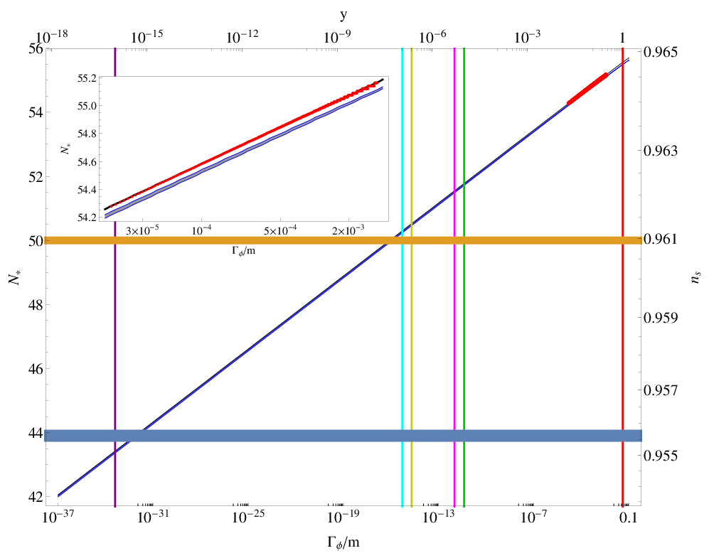
3.1 Decays via Superpotential Couplings
In one class of model discussed in [40], the inflaton was identified as an untwisted matter field in some suitable string compactification, with direct decays to matter particles via a Yukawa-like superpotential coupling. One possible realization of this scenario would be further to identify the inflaton as a singlet (right-handed) sneutrino with a couplings to light Higgs and lepton doublets [57, 31]. The perturbative decay rate of such a sneutrino inflaton would be given by (53) with identified as the neutrino Yukawa coupling . We use this as a representative of the broader class of matter inflatons that decay directly to matter particles via trilinear superpotential couplings.
Within the sneutrino inflation scenario, one might wish to consider values of , the upper limit corresponding to a value of the Yukawa coupling similar to that of the top quark. In this case, we estimate
| (54) |
as shown by the vertical red line in Fig. 7. However, such a large value of would reheat the Universe to a very high temperature GeV, which would lead to an overproduction of gravitinos whose decays could aversely affect big bang nucleosynthesis and could overpopulate the Universe with dark matter particles [58]. To avoid this overproduction, one should require . For the upper limit in this case, we estimate
| (55) |
as shown by the vertical green line in Fig. 7. On the other hand, as discussed above, the smallest value of consistent with conventional Big Bang nucleosynthesis is , in which case
| (56) |
as shown by the vertical purple line in Fig. 7. The above range of couplings includes possible gravitational decays of the inflaton §§ § As was discussed in [40], another possibility in such a matter inflaton scenario would be a superpotential coupling of the form , which would yield decays into fields with a rate . The results for different values of discussed below could also be applied to this case, by simply replacing . . We discuss below the compatibility of these predictions with the Planck data, shown as the horizontal yellow and blue lines in Fig. 7.
3.2 Decays via Gravitational-Strength Couplings
There is another class of no-scale models in which the the inflaton decays via couplings that are suppressed by one or more powers of , which we exemplify here by examples in which the compactification volume modulus is identified as the inflaton ¶¶ ¶ There are also matter-inflaton models in which decays are suppressed by some power of , but we do not discuss them here.. For instance, in the example discussed in Section 5.2 of [40], there are decays into three-body and related final states with rate
| (57) |
where and are modular weights that are . Since and , this example corresponds to
| (58) |
In this case we find
| (59) |
as shown by the vertical pale blue line in Fig. 7.
However, such three-body decays may be dominated by two-body inflaton decays into pairs of gauge bosons [59, 26], if the gauge kinetic function (where are gauge indices) has a non-trivial dependence on the volume modulus: with
| (60) |
which is a generic feature of heterotic string effective field theories. In this case, the decays into Standard Model gauge bosons yield
| (61) |
corresponding to
| (62) |
In a weakly-coupled heterotic string model, one might expect , whereas it might be in a strongly-coupled model, leading to
| (63) |
These estimates of lead to the following estimates of :
| (64) |
as shown by the vertical yellow and magenta lines in Fig. 7, respectively. The compatibility of these predictions with the Planck data is also discussed in the next Section.
4 CMB Bounds on in Representative No-Scale Inflation Models
4.1 Matter Inflaton Case
In the recent no-scale inflation model [29] with an untwisted matter field playing the role of the inflaton, the observables were calculated assuming a Kähler potential of the form (1) and choosing a Wess-Zumino superpotential combining bilinear and trilinear terms:
| (65) |
and assuming that the volume modulus is fixed. It was shown in [29] that this model reproduces exactly the predictions of the Starobinsky model if . This model can alternatively be written in a more symmetric form:
| (66) |
where
| (67) |
in which representation the superpotential (65) can be written as
| (68) |
In the Starobinsky limit , and we consider related models with .
The calculations of in the previous Sections were made assuming exactly Starobinsky-like inflation, which (as already mentioned) corresponds in this matter inflation model to the limiting case . We have studied the modification of the calculation when , but lying within the range displayed in Fig. 8.
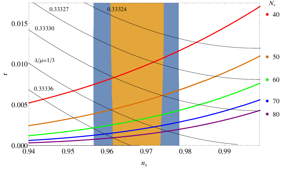
Fig. 8 displays the Planck 2015 constraints on this model in the plane (upper panel) and the plane (lower panel), with the region favoured at the 68% CL shaded yellow, and the region allowed at the 95% CL shaded blue. We see in the upper panel that for values of (black lines) the tensor to scalar ratio is small, and in this case, the data yield constraints on that are relatively insensitive to . On the other hand, we see that any fixed value of corresponds to values of (coloured lines) that are strongly correlated with the values of . Thus for a given value of , the lower bound on provided by Planck can be translated into a lower bound on that is sensitive to . For example, for , the 68% lower bound on corresponds to a lower bound of on .
This feature is reflected in the lower panel of Fig. 8, where we see that is essentially unconstrained in this model in the absence of a precise value for . However, if one assumes the Starobinsky value , one finds at the 68% CL, which would disfavour according to Fig. 7, and the 68% CL lower bound on would strengthen for .
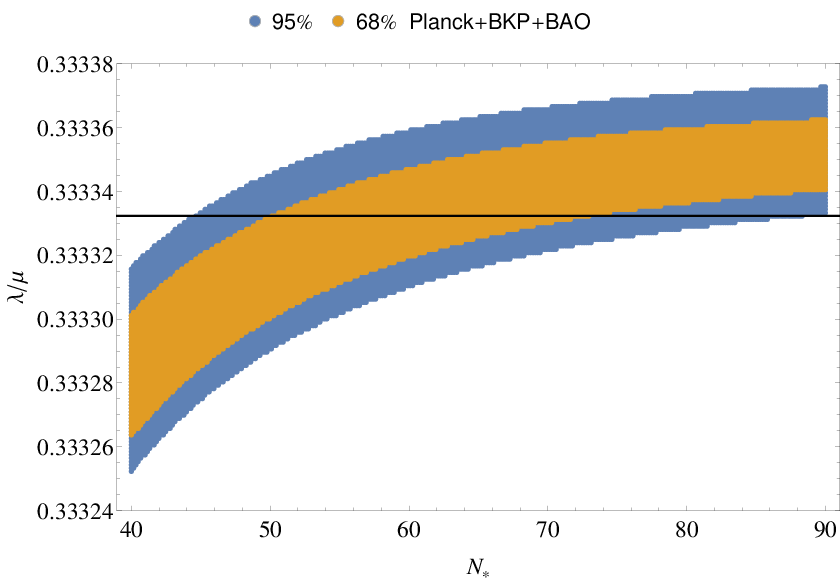
As seen in Fig. 9, the maximum deviation from the Starobinsky prediction for (as shown in Fig. 7) due to varying in the range studied (yellow band) is always , and the deviation is significantly smaller for the favoured models with inflaton decay via a two-body superpotential coupling (corresponding to the green vertical line in Fig. 7). The Starobinsky-like analysis gave for , as seen in (55), and the non-Starobinsky deviation of in Fig. 9 is for this value of , decreasing to much smaller values close to the Big Bang nucleosynthesis lower limit , for which we found in the Starobinsky limit, as seen in (56).

It is necessary to address in this model two potential issues: the stabilization of the real and imaginary parts of the field when the inflaton reaches its minimum, and the possibility that during inflation. The first of these issues is resolved by adding a small supplementary term to the superpotential (68):
| (69) |
for some constant . The second issue is addressed by incorporating a quartic term in the Kähler potential (66):
| (70) |
where typical values of in natural units, as discussed in [30].
Fig. 10 shows the 68% and 95% CL regions (yellow and blue, respectively) in the plane (upper panel) and in the plane (lower panel) for this no-scale inflationary model with the illustrative choice and the range . As shown in [30], this matter inflaton model reproduces the inflationary predictions of the Starobinsky model for , and we see in the upper panel of Fig. 10 that the data constraints on are insensitive to for in this range and the relevant values of (coloured lines). In each of the segments shown, varies from 1/100 to 1 as shown for several values of . Once again, we can use the lower bound on to derive a lower bound on for a given value of . Those limits are reproduced in the lower panel of Fig. 10 where we see that in the limit of small the current data require at the 95% CL and favour at the 68% CL. The variation in for values of is shown as a thin blue band in Fig. 9 as a function of . We see that this is always smaller than the variation due to varying , being and hence negligible for our purposes.


4.2 Volume Modulus Inflaton Cases
In [38, 39] we calculated the observables in various no-scale inflationary models in which the inflaton was identified with some combination of the real and imaginary parts of the complex volume modulus . In this case, we choose a superpotential of the form [60]
| (71) |
Inflation along the direction of the canonically normalized real component of yielded a Starobinsky-like model, whereas there was a quadratic potential along the imaginary direction [36, 37]. In [38] we assumed that higher-order terms in the Kähler potential fixed the angle of the inflationary trajectory in the complex plane, whereas [39] we made a complete two-field analysis of the inflationary observables and . We now confront these models with the Planck 2015 data.
The models are characterized by two parameters, the angle of the starting-point in the complex plane, which we parameterize here as ∥∥ ∥ Note that the angle used in [38, 39] is equivalent to ., and the modulus stabilization parameter [61]:
| (72) |
In this model the matter field relaxes dynamically to zero during inflation [38]. As was discussed in [38, 39], the case corresponds to a quadratic model of chaotic inflation, and smaller values of interpolate between this and the Starobinsky limit when . If the quartic stabilization term is large enough, the inflaton trajectory follows a narrow valley in field space, much like a bobsleigh run, whereas if is small the inflaton trajectory is less constrained and two-field effects become important. In this case, we found in [39] that the trajectories for tend to become more Starobinsky-like for smaller values of . Predictions of this model for various values of and , based on a full two-field analysis, can be found in [39], where it can be seen that the results depend on . The Planck 2015 68% and 95% CL contours in the plane can then be converted into the corresponding constraints on in these no-scale models as functions of and , as illustrated in the following figures.
In Fig. 11 we display the 68% and 95% CL regions (yellow and blue, respectively) in the plane (upper panel) and in the plane (lower panel) for the strongly-stabilized case **** ** Larger values of would give very similar results.. We see in the upper panel that in this case the data constraints on depend in an essential way on the value of , and we also see that the contours of (coloured lines) depend in a non-trivial way on the value of , as discussed in [39]. The interpolation between , the limit in which the model realizes chaotic quadratic inflation, and , the Starobinsky limit, is nonlinear.


For these reasons, the conversion of the CMB data into constraints on also depends non-trivially on , as seen in the “whale-like” shape in the lower panel of Fig. 11. In particular, the whale’s “mouth” is the converse of the leftward swerve in the contours in the upper panel of Fig. 11, and the “lower jaw” corresponds to the swerve back to larger at small . Overall, we see that is preferred at the 68% CL, whereas is allowed at the 95% CL. Translating these limits into constraints on is also less trivial than in the previous matter inflaton models, since this matter inflaton model is not Starobinsky-like for large , as seen in the upper panel of Fig. 11. As seen in Fig. 12, any fixed value of may correspond to a range of values of , shown by the blue band, depending on the value of . The upper side of the band correspond to the limit of chaotic inflation with a quadratic potential, and the lower side to the Starobinsky limit. As we see in Fig. 7, in the Starobinsky-like limit we find the following constraints on and the effective two-body coupling :
| (73) |
We have studied numerically the possible variations in the dependence of on the decay rate in the range , with the results shown as the blue band in Fig. 12. We see there that in the chaotic quadratic inflation case the constraint on is relaxed by a factor and the effective two-body coupling is relaxed correspondingly by a factor .

If , corresponding to values of as shown in (55) and Fig. 7 for the Starobinsky case, then only the range is allowed at the 68% CL, rising to at the 95% CL. Thus models with a starting-point of inflation with small close to the real direction, i.e., close to the Starobinsky model, are favoured in the strongly-stabilized case, though not strongly at the 95% CL. In the Starobinsky limit , corresponding to the lower jaw of the “whale” in Fig. 11, the value is at the Planck 2015 68% CL limit, whereas and hence is allowed at the 95% CL.
Fig. 13 shows analogous results for the unstabilized case . In this case, as seen in the upper panel, the important CMB constraint is that from , which is almost independent of for the relevant values of (coloured lines). The lower panel of Fig. 13 shows that again is favoured at the 68% CL, whereas now is allowed at the 95% CL. Both of these limits are rather insensitive to in the range , whereas only very large values of are allowed as , corresponding to a starting-point along the imaginary direction. In this case there is no significant preference for Starobinsky-like models with the starting-point of inflation close to the real direction.


Fig. 14 shows analogous results for inflation along the imaginary direction, i.e., , and allowing the stabilization parameter to vary. As we see in the upper panel, the cosmological constraint depends non-trivially on both and , and the values of these quantities for fixed (coloured lines) depend non-linearly on . In this case, as seen in the lower panel of Fig. 14, the lowest value of is found for , with favoured at the 68% CL and allowed at the 95% CL. As can be seen in Fig. 12, these constraints correspond to being favoured at the 68% CL, whereas all values of consistent with Big Bang nucleosynthesis are allowed at the 95% CL. This example shows that inflation is possible in this model even if the starting-point of inflation is close to the imaginary direction, far from the Starobinsky-like limit.


5 Summary and Prospects
The first purpose of this paper has been to present in Section 2 calculations of in models of inflaton decays, with particular attention to predictions in Section 3 from models that are motivated by no-scale models of inflation and have a structure inspired by common scenarios for string compactification. We have then analyzed in Section 4 the ranges of within no-scale models that yield values of and within the 68 and 95% CL regions found by the Planck Collaboration.
Comparing the results of the previous two Sections, we showed in detail how models with smaller inflaton decay rates lead to lower values of , and , whereas the data prefer larger values of and hence . Numerically, in the Starobinsky-like limit models with two-body decays and as suggested by the gravitino constraint correspond to , whereas the data favour at the 68% CL, with values of being allowed at the 95% CL. The present data therefore tend to favour models with relatively rapid inflaton decay: corresponding to for two-body decays at the 68% CL, to be compared with the upper bound from the gravitino abundance †††† †† However, the lower limit on may be relaxed by a factor (and that on by a factor ) in non-Starobinsky-like no-scale models.. It will be interesting to see how, as the experimental constraints tighten, the experimental noose on tightens ‡‡‡‡ ‡‡ The mild preference for rapid inflaton decay applies to many models, including the original Starobinsky model, no-scale Starobinsky-like models [29] and Higgs inflation.
It is interesting to consider specific messages from our analysis for a couple of phenomenological issues, namely sneutrino inflation and supersymmetry breaking.
The cosmological upper limit on the gravitino abundance imposes an upper limit on the Yukawa coupling responsible for sneutrino inflaton decay: , which is itself an important constraint on realizations of sneutrino inflation. If the matter field in the no-scale Wess-Zumino model (65) is identified with a sneutrino, it must have a trilinear coupling . Such a trilinear coupling violates -parity, inducing decay of the lightest supersymmetric particle. However, its lifetime is still much longer than the age of the Universe, and it remains a viable candidate for cold dark matter. As we have shown here, if , CMB measurements measurements favour , and hence are on the verge of providing a relevant lower bound on the coupling responsible for sneutrino decay. It will be interesting to see how this squeeze on will evolve.
Concerning supersymmetry breaking, we recall that there is a contribution to gaugino masses of the form
| (74) |
where is a number of order unity. We saw in Section 3 that strongly-coupled string models with would give larger values of the inflaton decay rate (62), and hence than weakly-coupled models with , as seen in (64). The difference in and hence is not yet significant, but this connection will also be interesting to watch in the future.
These two examples serve as illustrations how inflationary observables may in the future join the phenomenological mainstream. These two examples are in the context of specific no-scale supergravity models of inflation, but the connection has the potential to be more general.
Acknowledgements
The work of J.E. was supported in part by the London Centre for Terauniverse Studies (LCTS), using funding from the European Research Council via the Advanced Investigator Grant 267352 and from the UK STFC via the research grant ST/L000326/1. The work of D.V.N. was supported in part by the DOE grant DE-FG03- 95-ER-40917 and in part by the Alexander S. Onassis Public Benefit Foundation. The work of M.A.G.G. and K.A.O. was supported in part by DOE grant DE-SC0011842 at the University of Minnesota.
References
- [1] P. A. R. Ade et al. [Planck Collaboration], arXiv:1502.01589 [astro-ph.CO]; P. A. R. Ade et al. [Planck Collaboration], arXiv:1502.02114 [astro-ph.CO].
- [2] P. A. R. Ade et al. [BICEP2 and Planck Collaborations], Phys. Rev. Lett. 114, no. 10, 101301 (2015) [arXiv:1502.00612 [astro-ph.CO]].
- [3] J. Martin, C. Ringeval and V. Vennin, Phys. Dark Univ. 5-6, 75-235 (2014) [arXiv:1303.3787 [astro-ph.CO]]; J. Martin, C. Ringeval, R. Trotta and V. Vennin, JCAP 1403 (2014) 039 [arXiv:1312.3529 [astro-ph.CO]]; J. Martin, arXiv:1502.05733 [astro-ph.CO].
- [4] A. A. Starobinsky, Phys. Lett. B 91, 99 (1980).
- [5] V. F. Mukhanov and G. V. Chibisov, JETP Lett. 33, 532 (1981) [Pisma Zh. Eksp. Teor. Fiz. 33, 549 (1981)].
- [6] A. A. Starobinsky, Sov. Astron. Lett. 9, 302 (1983).
- [7] F. L. Bezrukov and M. Shaposhnikov, Phys. Lett. B 659, 703 (2008) [arXiv:0710.3755 [hep-th]].
- [8] J. R. Ellis, D. V. Nanopoulos, K. A. Olive and K. Tamvakis, Phys. Lett. B 118 (1982) 335; Phys. Lett. B 120 (1983) 331; Nucl. Phys. B 221 (1983) 52.
- [9] D. V. Nanopoulos, K. A. Olive, M. Srednicki and K. Tamvakis, Phys. Lett. B 123, 41 (1983); D. V. Nanopoulos, K. A. Olive and M. Srednicki, Phys. Lett. B 127, 30 (1983).
- [10] R. Holman, P. Ramond and G. G. Ross, Phys. Lett. B 137, 343 (1984).
- [11] A. B. Goncharov and A. D. Linde, Phys. Lett. B 139, 27 (1984).
- [12] E. J. Copeland, A. R. Liddle, D. H. Lyth, E. D. Stewart and D. Wands, Phys. Rev. D 49, 6410 (1994) [astro-ph/9401011]; E. D. Stewart, Phys. Rev. D 51, 6847 (1995) [hep-ph/9405389].
- [13] A. S. Goncharov and A. D. Linde, Class. Quant. Grav. 1, L75 (1984).
- [14] C. Kounnas and M. Quiros, Phys. Lett. B 151, 189 (1985).
- [15] J. R. Ellis, K. Enqvist, D. V. Nanopoulos, K. A. Olive and M. Srednicki, Phys. Lett. B 152 (1985) 175 [Erratum-ibid. 156B (1985) 452].
- [16] E. Cremmer, S. Ferrara, C. Kounnas and D. V. Nanopoulos, Phys. Lett. B 133 (1983) 61; J. R. Ellis, A. B. Lahanas, D. V. Nanopoulos and K. Tamvakis, Phys. Lett. B 134 (1984) 429.
- [17] A. B. Lahanas and D. V. Nanopoulos, Phys. Rept. 145 (1987) 1.
- [18] E. Witten, Phys. Lett. B 155 (1985) 151.
- [19] K. Enqvist, D. V. Nanopoulos and M. Quiros, Phys. Lett. B 159, 249 (1985).
- [20] P. Binétruy and M. K. Gaillard, Phys. Rev. D 34, 3069 (1986).
- [21] H. Murayama, H. Suzuki, T. Yanagida and J. Yokoyama, Phys. Rev. D 50, 2356 (1994) [arXiv:hep-ph/9311326].
- [22] S. C. Davis and M. Postma, JCAP 0803, 015 (2008) [arXiv:0801.4696 [hep-ph]].
- [23] S. Antusch, M. Bastero-Gil, K. Dutta, S. F. King and P. M. Kostka, JCAP 0901, 040 (2009) [arXiv:0808.2425 [hep-ph]]; S. Antusch, M. Bastero-Gil, K. Dutta, S. F. King and P. M. Kostka, Phys. Lett. B 679, 428 (2009) [arXiv:0905.0905 [hep-th]].
- [24] S. Antusch, K. Dutta, J. Erdmenger and S. Halter, JHEP 1104 (2011) 065 [arXiv:1102.0093 [hep-th]].
- [25] R. Kallosh and A. Linde, JCAP 1011, 011 (2010) [arXiv:1008.3375 [hep-th]]; R. Kallosh, A. Linde and T. Rube, Phys. Rev. D 83, 043507 (2011) [arXiv:1011.5945 [hep-th]].
- [26] R. Kallosh, A. Linde, K. A. Olive and T. Rube, Phys. Rev. D 84, 083519 (2011) [arXiv:1106.6025 [hep-th]].
- [27] T. Li, Z. Li and D. V. Nanopoulos, JCAP 1402, 028 (2014) [arXiv:1311.6770 [hep-ph]].
- [28] W. Buchmuller, C. Wieck and M. W. Winkler, arXiv:1404.2275 [hep-th].
- [29] J. Ellis, D. V. Nanopoulos and K. A. Olive, Phys. Rev. Lett. 111 (2013) 111301 [arXiv:1305.1247 [hep-th]].
- [30] J. Ellis, D. V. Nanopoulos and K. A. Olive, JCAP 1310 (2013) 009 [arXiv:1307.3537 [hep-th]];
- [31] J. Ellis, D. V. Nanopoulos and K. A. Olive, Phys. Rev. D 89, 043502 (2014) [arXiv:1310.4770 [hep-ph]].
- [32] F. Farakos, A. Kehagias and A. Riotto, Nucl. Phys. B 876, 187 (2013) [arXiv:1307.1137 [hep-th]].
- [33] W. Buchmüller, V. Domcke and C. Wieck, Phys. Lett. B 730, 155 (2014) [arXiv:1309.3122 [hep-th]].
- [34] C. Pallis, JCAP 1404, 024 (2014) [arXiv:1312.3623 [hep-ph]]; C. Pallis, JCAP 1408, 057 (2014) [arXiv:1403.5486 [hep-ph]].
- [35] I. Antoniadis, E. Dudas, S. Ferrara and A. Sagnotti, Phys. Lett. B 733, 32 (2014) [arXiv:1403.3269 [hep-th]].
- [36] S. Ferrara, A. Kehagias and A. Riotto, Fortsch. Phys. 62, 573 (2014) [arXiv:1403.5531 [hep-th]]; S. Ferrara, A. Kehagias and A. Riotto, Fortsch. Phys. 63, 2 (2015) [arXiv:1405.2353 [hep-th]].
- [37] J. Ellis, M. A. G. García, D. V. Nanopoulos and K. A. Olive, JCAP 1405, 037 (2014) [arXiv:1403.7518 [hep-ph]].
- [38] J. Ellis, M. A. G. García, D. V. Nanopoulos and K. A. Olive, JCAP 1408, 044 (2014) [arXiv:1405.0271 [hep-ph]].
- [39] J. Ellis, M. A. G. García, D. V. Nanopoulos and K. A. Olive, JCAP 1501, no. 01, 010 (2015) [arXiv:1409.8197 [hep-ph]].
- [40] J. Ellis, M. A. G. García, D. V. Nanopoulos and K. A. Olive, arXiv:1503.08867 [hep-ph].
- [41] T. Li, Z. Li and D. V. Nanopoulos, JCAP 1404, 018 (2014) [arXiv:1310.3331 [hep-ph]]; T. Li, Z. Li and D. V. Nanopoulos, Eur. Phys. J. C 75, no. 2, 55 (2015) [arXiv:1405.0197 [hep-th]].
- [42] S. Renaux-Petel and K. Turzynski, arXiv:1405.6195 [astro-ph.CO].
- [43] W. Buchmuller, E. Dudas, L. Heurtier and C. Wieck, JHEP 1409, 053 (2014) [arXiv:1407.0253 [hep-th]]; W. Buchmuller, E. Dudas, L. Heurtier, A. Westphal, C. Wieck and M. W. Winkler, JHEP 1504, 058 (2015) [arXiv:1501.05812 [hep-th]].
- [44] C. Kounnas, D. Lüst and N. Toumbas, Fortsch. Phys. 63, 12 (2015) [arXiv:1409.7076 [hep-th]].
- [45] T. Terada, Y. Watanabe, Y. Yamada and J. Yokoyama, JHEP 1502, 105 (2015) [arXiv:1411.6746 [hep-ph]].
- [46] A. B. Lahanas and K. Tamvakis, Phys. Rev. D 91, no. 8, 085001 (2015) [arXiv:1501.06547 [hep-th]].
- [47] I. Dalianis and F. Farakos, arXiv:1502.01246 [gr-qc].
- [48] D. Roest and M. Scalisi, arXiv:1503.07909 [hep-th].
- [49] J. Martin and C. Ringeval, Phys. Rev. D 82, 023511 (2010) [arXiv:1004.5525 [astro-ph.CO]].
- [50] J. Mielczarek, Phys. Rev. D 83, 023502 (2011) [arXiv:1009.2359 [astro-ph.CO]]; R. Easther and H. V. Peiris, Phys. Rev. D 85, 103533 (2012) [arXiv:1112.0326 [astro-ph.CO]]; L. Dai, M. Kamionkowski and J. Wang, Phys. Rev. Lett. 113, 041302 (2014) [arXiv:1404.6704 [astro-ph.CO]]; J. Martin, C. Ringeval and V. Vennin, Phys. Rev. Lett. 114, no. 8, 081303 (2015) [arXiv:1410.7958 [astro-ph.CO]]; J. B. Munoz and M. Kamionkowski, Phys. Rev. D 91, no. 4, 043521 (2015) [arXiv:1412.0656 [astro-ph.CO]]; J. O. Gong, S. Pi and G. Leung, JCAP 1505, no. 05, 027 (2015) [arXiv:1501.03604 [hep-ph]]; J. L. Cook, E. Dimastrogiovanni, D. A. Easson and L. M. Krauss, JCAP 1504, no. 04, 047 (2015) [arXiv:1502.04673 [astro-ph.CO]].
- [51] A. R. Liddle and S. M. Leach, Phys. Rev. D 68, 103503 (2003) [astro-ph/0305263].
- [52] S. M. Leach, A. R. Liddle, J. Martin and D. J. Schwarz, Phys. Rev. D 66, 023515 (2002) [astro-ph/0202094].
- [53] F. Finelli, J. Hamann, S. M. Leach and J. Lesgourgues, JCAP 1004, 011 (2010) [arXiv:0912.0522 [astro-ph.CO]].
- [54] A. R. Liddle, P. Parsons and J. D. Barrow, Phys. Rev. D 50, 7222 (1994) [astro-ph/9408015].
- [55] M. S. Turner, Phys. Rev. D 28, 1243 (1983).
- [56] S. Davidson and S. Sarkar, JHEP 0011, 012 (2000) [hep-ph/0009078]; K. Harigaya and K. Mukaida, JHEP 1405, 006 (2014) [arXiv:1312.3097 [hep-ph]]; M. A. Amin, M. P. Hertzberg, D. I. Kaiser and J. Karouby, Int. J. Mod. Phys. D 24, no. 01, 1530003 (2014) [arXiv:1410.3808 [hep-ph]].
- [57] H. Murayama, H. Suzuki, T. Yanagida and J.-i. Yokoyama, Phys. Rev. Lett. 70 (1993) 1912 and Phys. Rev. D 50 (1994) 2356 [hep-ph/9311326]; J. R. Ellis, M. Raidal and T. Yanagida, Phys. Lett. B 581 (2004) 9 [hep-ph/0303242]; D. Croon, J. Ellis and N. E. Mavromatos, Phys. Lett. B 724 (2013) 165 [arXiv:1303.6253 [astro-ph.CO]]; K. Nakayama, F. Takahashi and T. T. Yanagida, Phys. Lett. B 730, 24 (2014) [arXiv:1311.4253 [hep-ph]]; J. Ellis, N. E. Mavromatos and D. J. Mulryne, JCAP 1405 (2014) 012 [arXiv:1401.6078 [astro-ph.CO]]; J. L. Evans, T. Gherghetta and M. Peloso, arXiv:1501.06560 [hep-ph].
- [58] M. Bolz, A. Brandenburg and W. Buchmuller, Nucl. Phys. B 606, 518 (2001) [Erratum-ibid. B 790, 336 (2008)] [hep-ph/0012052]; R. H. Cyburt, J. Ellis, B. D. Fields and K. A. Olive, Phys. Rev. D 67, 103521 (2003) [astro-ph/0211258]; F. D. Steffen, JCAP 0609, 001 (2006) [hep-ph/0605306]; M. Kawasaki, K. Kohri, T Moroi and A.Yotsuyanagi, Phys. Rev. D 78, 065011 (2008) [arXiv:0804.3745 [hep-ph]]; R. H. Cyburt, J. Ellis, B. D. Fields, F. Luo, K. A. Olive and V. C. Spanos, JCAP 0910, 021 (2009) [arXiv:0907.5003 [astro-ph.CO]]; R. H. Cyburt, J. Ellis, B. D. Fields, F. Luo, K. A. Olive and V. C. Spanos, JCAP 1305, 014 (2013) [arXiv:1303.0574 [astro-ph.CO]].
- [59] M. Endo, K. Kadota, K. A. Olive, F. Takahashi and T. T. Yanagida, JCAP 0702, 018 (2007) [hep-ph/0612263].
- [60] S. Cecotti, Phys. Lett. B 190 (1987) 86.
- [61] J. R. Ellis, C. Kounnas and D. V. Nanopoulos, Phys. Lett. B 143, 410 (1984).