On the Peterlin approximation for turbulent flows of polymer solutions
Abstract
We study the impact of the Peterlin approximation on the statistics of the end-to-end separation of polymers in a turbulent flow. The FENE and FENE-P models are numerically integrated along a large number of Lagrangian trajectories resulting from a direct numerical simulation of three-dimensional homogeneous isotropic turbulence. Although the FENE-P model yields results in qualitative agreement with those of the FENE model, quantitative differences emerge. The steady-state probability of large extensions is overestimated by the FENE-P model. The alignment of polymers with the eigenvectors of the rate-of-strain tensor and with the direction of vorticity is weaker when the Peterlin approximation is used. At large Weissenberg numbers, both the correlation times of the extension and of the orientation of polymers are underestimated by the FENE-P model.
I Introduction
The addition of elastic polymers to a Newtonian solvent introduces a history dependence in the response of the fluid to a deformation and hence modifies the rheological properties of the solvent. [1] In turbulent flows, the non-Newtonian nature of polymer solutions manifests itself through a considerable reduction of the turbulent drag compared to that of the solvent alone. [2, 3, 4, 5, 6] What renders this phenomenon even more remarkable is that an appreciable drag reduction can already be observed at very small polymer concentrations (of the order of a few parts per million). Turbulent drag reduction was discovered by Toms [7] more than sixty years ago and is nowadays routinely used to reduce energy losses in crude-oil pipelines. [8] A full understanding of turbulent drag reduction nonetheless remains a difficult challenge, because in the turbulent flow of a polymer solution the extensional dynamics of a large number of polymers is coupled with strongly nonlinear transfers of kinetic energy.
The study of turbulent flows of polymer solutions is essentially based on two approaches: the molecular approach and the continuum one. In the molecular (or Brownian Dynamics) approach, a polymer is modeled as a sequence of beads connected by elastic springs. The deformation of the bead-spring chain is then followed along the trajectory of its center of mass. In homogeneous and isotropic turbulence, Watanabe and Gotoh [9] have shown that beads are in fact sufficient to describe the stationary statistics of both the extension and the orientation of polymers, i.e., the deformation of a polymeric chain is dominated by its slowest oscillation mode. An analogous conclusion has been reached by Terrapon et al. [13] in a study of polymer dynamics in a turbulent channel flow. The model consisting of only beads is known as the finitely extensible nonlinear elastic (FENE) dumbbell model. [1] The molecular approach is suitable for studying the deformation of passively transported polymers [10, 11, 12, 13, 14, 15, 16, 17, 18, 19, 9, 20, 21]. Two-way coupling molecular simulations are a recent achievement [22, 23, 24] and have not yet been employed in practical applications owing to their computational cost. In the molecular approach, indeed, the feedback of polymers on the velocity field is given by the forces exerted on the fluid by a huge number of polymeric chains. [22, 23, 24]
For the above reason, in practical applications, numerical simulations of turbulent flows of polymer solutions generally use the continuum approach. The conformation of polymers is then described by means of a space- and time-dependent tensor field, which represents the average inertia tensor of polymers at a given time and position in the fluid. Such tensor is termed the polymer conformation tensor. An evolution equation for the conformation tensor may in principle be derived from the FENE dumbbell model. Such equation, however, involves the average over thermal fluctuations of a nonlinear function of the polymer end-to-end vector; a closure approximation is therefore required. Peterlin [25] proposed a mean-field closure according to which the average of the elastic force over thermal fluctuations is replaced by the value of the force at the mean-squared polymer extension. The resulting model was subsequently dubbed the FENE-P model.[26] Within the FENE-P model, the back-reaction of polymers on the flow is described by a stress tensor field, which depends on the polymer conformation tensor. This continuum model is thus suitable for simulating turbulent flows of polymer solutions; it indeed amounts to simultaneously solving the evolution equation for the polymer conformation tensor and the Navier–Stokes equation with an additional elastic-stress term. The FENE-P model is widely employed in numerical simulations of turbulent drag reduction and has been successfully applied to channel flows, [27, 28, 29, 30] shear flows, [31, 32] and two- and three-dimensional homogeneous and isotropic turbulence.[33, 34, 35, 36] Nevertheless, although it qualitatively reproduces the main features of turbulent drag reduction, the FENE-P model generally does not yield results in quantitative agreement with experimental data (e.g. Ref. 30). It is therefore essential to assess the validity of the assumptions on which the model is based.
For laminar flows, the Peterlin approximation has been examined in detail (see Refs. 37, 38 and references therein). In particular, the FENE-P model is a good approximation of the FENE model in steady flows, whereas appreciable differences appear in time-dependent flows. This observation suggests that in turbulent flows important differences between the two models should be expected. Several studies have subsequently investigated the validity of the Peterlin approximation in turbulent flows by comparing one-way coupling simulations of the FENE and FENE-P models.[11, 12, 13, 15, 19] These studies have clearly shown potential differences among FENE and FENE-P models together with high sensitivity on the statistical ensemble and dependency on the degree of homogeneity of the underlying velocity fluctuations. We undertake a systematic analysis of the Peterlin approximation in three-dimensional homogeneous and isotropic turbulence by means of one-way coupling Lagrangian simulations of the FENE and FENE-P models. The size of our statistical ensemble ( fluid trajectories and realizations of thermal noise per trajectory) allows us to fully characterize the statistics of polymer extension and orientation. When the flow is turbulent two independent effects are at the origin of the discrepancies between the FENE and FENE-P models: one is directly related to the closure approximation for the elastic force, while the other is of a statistical nature and is a consequence of deriving the statistics of polymer deformation from that of the conformation tensor. By isolating these two effects, we compare the steady-state statistics and the temporal correlation of the extension and of the orientation of polymers in the FENE and in the FENE-P model.
II FENE and FENE-P models
In the FENE model, a polymer is described as two beads connected by an elastic spring, i.e., as an elastic dumbbell. [1] If the fluid is at rest, the polymer is in a coiled configuration because of entropic forces and its equilibrium extension is determined by the intensity of thermal fluctuations. If the polymer is introduced in a moving fluid and the velocity field changes over the size of the polymer, then the polymer can stretch and deform. The dynamics of the polymer thus results from the interplay between the stretching action of the velocity gradient and the elastic force, which tends to take the polymer back to its equilibrium configuration.
The maximum extension of the dumbbell is assumed to be smaller than the Kolmogorov scale, so that the velocity field changes linearly in space at the scale of the dumbbell. The drag force on the beads is given by the Stokes law. Moreover, inertial effects and hydrodynamical interactions between the beads are disregarded. Polymer–polymer hydrodynamical interactions are also disregarded under the assumption that the polymer concentration is very low. Thus, the separation vector between the beads, , satisfies the following stochastic ordinary differential equation (the FENE equation): [1, 39]
| (1) |
where , is the velocity gradient at the position of the center of mass of the dumbbell, is three-dimensional white noise, is the polymer root-mean-square equilibrium extension, and is the polymer relaxation time ( is the time scale that describes the exponential relaxation of to its equilibrium value in the absence of flow). The three terms on the right-hand-side of Eq. (1) represent the stretching by the velocity gradient, the restoring elastic force, and thermal noise, respectively. The function determines the elastic force and, in the FENE model, it has the following form:
| (2) |
where is the maximum extension of the polymer. The elastic force diverges as approaches ; hence extensions greater than are forbidden. Note that is a random vector and that, when is turbulent, two independent sources of randomness influence its evolution: thermal noise and the velocity gradient itself.
The polymer conformation tensor is defined as , where denotes an average over thermal fluctuations. To derive the evolution equation for , we apply the Itô formula to and use Eq. (1):
| (3) |
Whereas there is no Itô–Stratonovich ambiguity for Eq. (1), Eq. (3) should be understood in the Itô sense. We now average Eq. (3) with respect to the realizations of and make use of the following property of the Itô integral: . We thus obtain:
| (4) |
Equation (4) is not closed with respect to because of the term:
| (5) |
To obtain a closed equation, Peterlin [25] proposed the following approximation:
| (6) |
The resulting evolution equation for the polymer conformation tensor (the FENE-P equation) is:
| (7) |
where is the identity matrix and denotes the polymer conformation tensor calculated according to the Peterlin approximation. If the flow is turbulent, both and have a random behavior. In the following, we shall denote:
| (8) |
Equation (7) describes the evolution of the conformation tensor of a polymer along the Lagrangian trajectory of its center of mass. Numerical simulations of drag reduction use the Eulerian counterpart of Eq. (7), which is obtained by replacing with and with the Eulerian velocity gradient. In principle, the evolution equation for the conformation tensor should be coupled with the Navier–Stokes equations through an additional stress term proportional to . [1] Here, however, we focus on the impact of the Peterlin approximation upon the statistics of polymer deformation and consider passive polymers only (one-way coupling). In the rest of the paper, we thus study the relation between Eq. (7) and Eq. (1) when is given by the incompressible Navier–Stokes equations in the turbulent regime. Some considerations are useful to guide our study:
- 1.
- 2.
because of the Peterlin approximation (Eq. (6)), the FENE and FENE-P equations yield a different evolution for the conformation tensor. This holds for both laminar and turbulent flows;
- 3.
If the flow is turbulent, the statistics of differs from that of , even if is calculated from Eq. (1) (and hence no closure approximation is required). Consider for example the random variables and . In general, the probability density function (PDF) of is different from that of , as can be seen by noting that (), where denotes an average over the statistics of the turbulent velocity gradient.
In conclusion, the FENE and FENE-P models differ for two reasons: the Peterlin approximation and the statistical effect due to the fact that the statistics of cannot be deduced from that of . Hence, in the turbulent regime, the proper way to examine the Peterlin approximation is to first construct from the FENE equation and then compare its statistics with that of the solution of the FENE-P equation. If the statistics of is directly compared with that of , the error due to the Peterlin approximation is combined with the statistical effect discussed at point 3 above. This fact seems to have been overlooked in previous studies.
III Lagrangian simulations
The dynamics of polymers is studied by using a database of Lagrangian trajectories that was previously generated to examine the dynamics of both tracer and inertial particles in turbulent flows. [40, 41] The turbulent velocity field is obtained by direct numerical simulation of the three-dimensional incompressible Navier–Stokes equations:
| (9) |
where is the pressure field and is the kinematic viscosity. The forcing is such that the spectral content of the first low-wavenumber shells remains constant in time. The domain is a three-dimensional periodic box of linear size . Equations (9) are solved by means of a fully dealiased pseudospectral algorithm with second-order Adams–Bashforth time stepping. The number of grid points is , while the integration time step is . In this simulation, the Kolmogorov time is and the Taylor-microscale Reynolds number is (for more details on the numerical simulation, see Refs. 40, 41). We expect our results not to depend significantly on the value of except for some residual effects induced by intermittency in the statistics of the velocity gradients. [42]
As mentioned in Sect. II, the inertia of polymers is negligible. Furthermore, their thermal diffusivity is very small compared to the turbulent diffusivity. Hence the center of mass of a polymer moves like a tracer and its position satisfies the following equation:
| (10) |
Equation (10) is once again solved by using a second-order Adams–Bashforth scheme; a tri-linear interpolation algorithm is used to determine the value of the velocity field at the position of the polymer. [40, 41] After the statistically stationary state is reached for both the fluid motion and the translational dynamics of polymers, the positions of the center of mass of polymers are recorded every . The total integration time after steady-state is , which corresponds to 6 eddy turnover times approximately.
The velocity gradient is recorded every along the trajectory of the center of mass of each polymer and is inserted into Eqs. (1) and (7) in order to determine the dynamics of the separation vector and of the conformation tensor. Equation (1) is solved by using the semi-implicit predictor–corrector method introduced by Öttinger; [39] the integration time step is equal to for all values of the parameters. The initial condition for Eq. (1) is such that , . Equation (7) for is integrated by means of the semi-implicit algorithm proposed in Ref. 13, which ensures that .
The Weissenberg number is defined as and is the ratio of the time scales associated with the elastic force and with the velocity gradient. In our simulations, varies between and . (An alternative definition of the Weissenberg number uses the maximum Lyapunov exponent of the flow, , to estimate the reciprocal of the stretching time associated with the velocity gradient. In our simulations, . [43] Thus, the Weissenberg number based on the Lyapunov exponent is ). The squares of the equilibrium and maximum extensions of the polymer are and , as in Refs. 19, 9. The number of realizations of thermal noise per Lagrangian trajectory is .
Finally, the statistics of polymer deformation is collected over the Lagrangian trajectories, over the realizations of thermal noise, and over time (only for times greater than the time required for to reach the statistically steady state).
We note that the statistics of the separation vector in isotropic turbulence has been studied thoroughly by Watanabe and Gotoh. [9] The results on the statistics of given below agree with those presented in Ref. 9. Here, we compare the statistics of with that of , in order to determine the effect of the Peterlin approximation on the dynamics of polymers.


IV Results
In this Section, we examine the statistics of polymer extension and orientation in the FENE and FENE-P models. Before presenting the results, it is useful to define some notations. If the statistics of a random variable depends both on thermal noise and on the velocity gradient (as for instance in the case of ), its PDF is denoted as . If the statistics of a random variable (e.g., ) only depends on the velocity gradient, then its PDF is denoted as . The auto-correlation function of a scalar random variable is denoted as and the correlation time of is: . The auto-correlation function of a statistically isotropic, unit random vector is defined as:
| (11) |
and the associated correlation time is defined as: . We denote by () the unit eigenvectors of the rate-of-strain tensor ; the unit eigenvectors are ordered by descending eigenvalue, i.e. is associated with the largest eigenvalue of and with the smallest one. The direction of vorticity is . Finally, we denote by and the first unit eigenvector of and , respectively.
IV.1 The Peterlin approximation
As mentioned in Sect. II, the Peterlin approximation consists in replacing with in the evolution equation for the polymer conformation tensor ( and have been defined in Eqs. (6) and (8) and, up to a concentration-dependent multiplicative constant, are the polymer stress tensors in the FENE and in the FENE-P models, respectively). The eigenvectors of and are the same, but their eigenvalues may differ. Indeed, Jensen’s inequality yields: . A first indication of the effect of the Peterlin approximation is thus given by the joint PDF (see Fig. 1). For small polymer extensions or for small values of , and are approximately the same because ; hence the Peterlin approximation holds very well. By contrast, for large extensions or for large values of , the deviations of from are significant, i.e. the Peterlin approximation is poor. Notwithstanding, and do not differ appreciably (see the bottom, right panel in Fig. 1). This fact demonstrates that the study of average values may not suffice to investigate the validity of the Peterlin approximation. The full statistics of the separation vector and the conformation tensor should be investigated, which requires following the Lagrangian dynamics of a large number of polymers.
In addition, the qualitative behavior of the temporal autocorrelations of and are similar (Figs. 2(a) to 2(c)), but for large the correlation time of is shorter than that of (Fig. 2(d)).


IV.2 Statistics of polymer extension


The statistical properties of the separation are well understood. For small values of , most of polymers are in the coiled state, i.e. their extension is close to the equilibrium one. Accordingly, the PDF of has a pronounced peak at . As increases, polymers unravel and become more and more extended. The transition from the coiled to the stretched state occurs when the Lyapunov exponent of the flow exceeds , i.e. at . [44] (Note that some authors define the Weissenberg number in terms of the time scale associated with the exponential relaxation of instead of and hence obtain a critical Weissenberg number equal to unity.)
At intermediate extensions, the PDF of has a power-law behavior, i.e. for . [44] This property of indicates that polymers with very different extensions coexist in the fluid; whether the coiled or the stretched state dominates depends on the value of . The exponent is positive in the coiled state and decreases as a function of . [44, 9, 20, 45] As long as , the FENE dumbbell model reaches a steady-state even as tends to infinity (the limit of the FENE model is known as the Hookean model [1]). However, when vanishes a steady-state PDF of the extension no longer exists if . This behavior is interpreted as the coil–stretch transition. [44] Finally, if increases beyond the value of the coil–stretch transition, becomes negative and the maximum of moves from close to to close to .[45, 9] The statistics of is shown in Figs. 3 and 4 for different values of .
We noted in Sect. II that the comparison between the FENE and the FENE-P model ought to be done in terms of the conformation tensors and (rather than in terms of and ). Let us denote and . To examine the influence of the Peterlin approximation on the statistics of polymer extension, we calculate from the solution of Eq. (1) and from Eq. (7). We then compare and in the steady state for different values of . The plots shown in Figs. 3 and 4 correspond to the coiled state (), the coil–stretch transition (), and the stretched state ().

For small values of , and do not differ significantly, because the extension of most of polymers is near to and hence and (Fig. 3(a)). For intermediate and large values of , the statistics of is characterized by a broad distribution of extensions around the mean value. The differences between and , therefore, are considerable. In particular, since is appreciably less than even for the largest and rapidly diverges for close to [see Eq. (2)], the restoring term in Eq. (7) is weaker than that in Eq. (1). Hence, in the FENE-P model large extensions are more probable than in the FENE model to the detriment of small and intermediate extensions (Fig. 3(b) and (c)). As a consequence, the FENE-P model overestimates the average extension of polymers for large values of (Fig. 3(d)). An analogous behavior of the average extension has been observed in turbulent channel flows. [13, 15]
We also note that whereas for large the PDFs of and are approximately the same (Fig. 3(c)), they are significantly different for intermediate or small (Figs. 3(a) and (b)). Indeed, in the former case, the stretching action of the velocity gradient is very strong compared to the effect of thermal fluctuations, and in most realizations . In the latter case, the effect of thermal fluctuations cannot be disregarded and the differences in the statistics of and (see Sect. II) become evident. Furthermore, and mainly differ for small and intermediate extensions, because the large extensions are obtained in those realizations in which the velocity gradient is very intense and thermal noise can be neglected. The above results demonstrate that comparing the statistics of directly with that of may lead to wrong conclusions; indeed, at small , and are clearly different, whereas and are close.
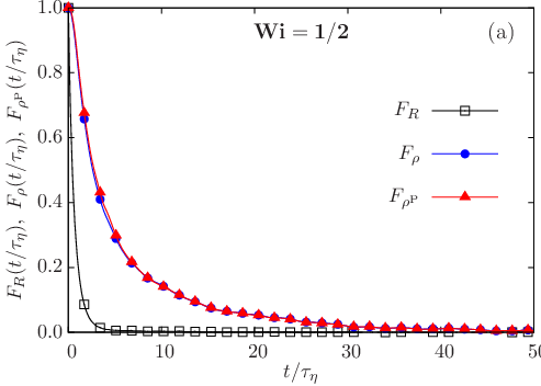
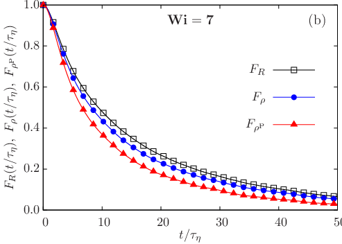
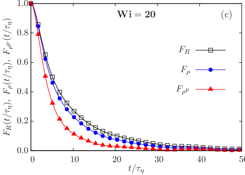
The autocorrelation function of the extension is approximately exponential both in the FENE and in the FENE-P model. However, is a good approximation of only for small (Fig. 5(a)). In addition, the FENE-P model captures the critical slowing down of polymers near the coil–stretch transition, [17, 46, 47] but for large it underestimates the correlation time of the extension (Fig. 5(d)). Once again, we note that, for small , a direct comparison between and would lead to wrong conclusions about the effect of the Peterlin approximation on the temporal statistics of polymer extension.
IV.3 Statistics of polymer orientation


In a coupled simulation of turbulent drag reduction, the feedback of polymers on the flow is of a tensorial nature; therefore, it depends not only on the extension of polymers but also on their orientation.
For small values of , the separation vector exhibits a weak alignment with the eigendirections of the rate-of-strain tensor or with the vorticity, [9] because thermal fluctuations (which are isotropic) strongly affect the dynamics. In contrast, for intermediate or large values of , thermal fluctuations have a negligible effect on the dynamics of polymers. Consequently, the evolution of the extension decouples from that of the orientation , which behaves like the orientation vector of a rigid rod and is the solution of the Jeffery equation. [48] For , the statistics of is therefore independent of and coincides with that of the orientation of a rigid rod, i.e. exhibits a moderate alignment with and a strong alignment with (see Refs. 19, 9, 49 and Fig. 6).
In the FENE-P model, the first eigenvector of , i.e. , can be interpreted as the orientation of the polymer, provided is sufficiently large. The effect of the Peterlin approximation on polymer orientation can then be studied by comparing the statistics of with that of the first eigenvector of . Fig. 6 shows that the FENE-P model qualitatively reproduces the statistics of polymer orientation but underestimates the level of alignment.
The autocorrelation function of decays exponentially (Figs. 7(a) to 7(c)), which for large is in agreement with the results for the autocorrelation of the orientation of a rod. [49] The correlation time of increases for small values of and saturates at large (Fig. 7(d)), because for large values of the Weissenberg number the dynamics of the orientation of becomes independent of . The FENE-P model agrees with the FENE model at small , but quantitative discrepancies appear at large (Figs. 7(a) to 7(c)). In particular, the FENE-P model underestimates the correlation time of polymer orientation (Figs. 7(d).
V Conclusions
Numerical simulations of turbulent flows of polymer solutions use the FENE-P model, which is based on the elastic dumbbell model but requires a closure approximation for the elastic term. We have examined the effect of the Peterlin approximation on the steady-state statistics of the extension and the orientation of polymers. The FENE-P model captures the qualitative properties of the statistics, but for large it underestimates the steady-state probability of small extensions and overestimates the probability of large extensions. As a consequence, the Peterlin approximation yields a greater average extension as well as a greater probability that polymers break under the action of a turbulent flow. [50] To quantify this effect, one would need to couple the dynamics of polymers with a fragmentation model connected to the accumulated (or instantaneous) stress along each trajectory and to estimate the relative breaking rate. [51] Since large polymer extensions are more likely in the FENE-P model than in the FENE model, we also expect that the Peterlin approximation yields a stronger feedback of polymers on the flow in two-way coupling simulations of homogeneous isotropic turbulence with polymer additives. A similar argument, however, does not carry over to inhomogeneous flows like channel flows. In this case, indeed, drag reduction is caused by the strong stretching of polymers in the near wall region rather than by the dynamics in the bulk of the channel, where the flow is homogeneous and isotropic and a lower degree of stretching is observed.[2, 11, 12, 13, 14, 21]
As regards the temporal statistics of the end-to-end separation vector, both the correlation times of the extension and the orientation of polymers are underestimated by the FENE-P model. The FENE-P model also underestimates the level of alignment of polymers with the eigenvectors of the rate-of-strain tensor and with the direction of vorticity.
It would be interesting to check to what extent these properties of the FENE-P model influence the dynamics of a polymer solution by comparing two-way coupling simulations of the FENE-P model in which the stress tensor is either calculated according to the Peterlin approximation or from molecular dynamics.
In this paper, we examined the Peterlin approximation, as this is the main assumption in the construction of a continuum model of polymer solutions. However, it is worth recalling that the FENE-P model is based on the dumbbell model and hence on a very simplified coarse-grained description of a polymer macromolecule. Other approximations may thus impact the performance of the FENE-P model and its comparison with experiments. For instance, even for simple laminar flows, the dumbbell model reproduces the experimental observations only if the maximum extension and the effective bead radius are used as free parameters to fit the experimental data.[52, 53]
Acknowledgements.
This work was supported in part by the EU COST Action MP1305 “Flowing Matter” and by a research program of the Foundation for Fundamental Research on Matter (FOM), which is part of the Netherlands Organisation for Scientific Research (NWO). Part of the computations were done at “Mésocentre SIGAMM,” Observatoire de la Côte d’Azur, Nice, France. DV acknowledges the hospitality of the Department of Physics of the Eindhoven University of Technology, where part of this work was done, and the Indo–French Centre for Applied Mathematics (IFCAM), Bangalore, for financial support.References
- [1] R.B. Bird, O. Hassager, R.C. Armstrong, and C.F. Curtiss, Dynamics of Polymeric Liquids, vol. 2 (John Wiley and Sons, Inc., 1977).
- [2] I. Procaccia, V.S. L’Vov, and R. Benzi, “Theory of drag reduction by polymers in wall-bounded turbulence,” Rev. Mod. Phys. 80, 225–247 (2008).
- [3] C.M. White and M.G. Mungal, “Mechanics and prediction of turbulent drag reduction with polymer additives,” Annu. Rev. Fluid Mech. 40, 235–256 (2008).
- [4] R. Pandit, P. Perlekar and S.S. Ray, “Statistical properties of turbulence: An overview,” Pramana – Journal of Physics, 73, 157–191 (2009).
- [5] R. Benzi, “A short review on drag reduction by polymers in wall bounded turbulence,” Physica D 239, 1338–1345 (2010).
- [6] M.D. Graham, “Drag reduction and the dynamics of turbulence in simple and complex fluids,” Phys. Fluids 26, 101301 (2014).
- [7] B.A. Toms, “Some observations on the flow of linear polymer solutions through straight tubes at large Reynolds numbers,” in Proceedings of the 1st International Congress on Rheology (North-Holland, Amsterdam, 1949), Vol. 2, pp. 135–141.
- [8] A. Gyr and H.-W. Bewersdorff, Drag Reduction of Turbulent Flows by Additives (Kluwer Academic Publishers, Dordrecht, 1995).
- [9] T. Watanabe and T. Gotoh, “Coil–stretch transition in an ensemble of polymers in isotropic turbulence,” Phys. Rev. E 81, 066301 (2010).
- [10] H. Massah, K. Kontomaris, W.R. Schowalter, and T.J. Hanratty, “The configuration of a FENE bead-spring chain in transient rheological flows and in a turbulent flow,” Phys. Fluids A 5, 881–890 (1993).
- [11] P. Ilg, E. De Angelis, I.V. Karlin, C.M. Casciola, and S. Succi, “Polymer dynamics in wall turbulent flow,” Europhys. Lett. 58, 616–622 (2002).
- [12] Q. Zhou and R. Akhavan, “A comparison of FENE and FENE-P dumbbell and chain models in turbulent flow,” J. Non-Newtonian Fluid Mech. 109, 115-155 (2003).
- [13] V.E. Terrapon, Y. Dubief, P. Moin, and E.S.G. Shaqfeh, “Brownian dynamics simulation in a turbulent channel flow,” in Proceedings of ASME, ASME/JSME 4th Joint Fluids Engineering Conference (FEDSM2003) (Honolulu, Hawaii, USA, July 6–10, 2003), pp. 773–780.
- [14] V.E. Terrapon, Y. Dubief, P. Moin, E.S.G. Shaqfeh, and S.K. Lele, “Simulated polymer stretch in a turbulent flow using Brownian dynamics,” J. Fluid Mech. 504, 61–71 (2004).
- [15] V.K. Gupta, R. Sureshkumar, and B. Khomami, “Polymer chain dynamics in Newtonian and viscoelastic turbulent channel flows,” Phys. Fluids 16, 1546–1566 (2004).
- [16] A. Celani, S. Musacchio, and D. Vincenzi, “Polymer transport in random flow,” J. Stat. Phys. 118, 531–554 (2005).
- [17] A. Celani, A. Puliafito, and D. Vincenzi, “Dynamical slowdown of polymers in laminar and random flows,” Phys. Rev. Lett. 97, 118301 (2006).
- [18] J. Davoudi and J. Schumacher, “Stretching of polymers around the Kolmogorov scale in a turbulent shear flow,” Phys. Fluids 18, 025103 (2006).
- [19] S. Jin and L.R. Collins, “Dynamics of dissolved polymer chains in isotropic turbulence,” New J. Phys. 9, 360 (2007).
- [20] S. Musacchio and D. Vincenzi, “Deformation of a flexible polymer in a random flow with long correlation time,” J. Fluid Mech. 670, 326 (2011).
- [21] F. Bagheri, D. Mitra, P. Perlekar, and L. Brandt, “Statistics of polymer extensions in turbulent channel flow,” Phys. Rev. E 86, 056314 (2012).
- [22] T. Peters and J. Schumacher, “Two-way coupling of finitely extensible nonlinear elastic dumbbells with a turbulent shear flow,” Phys. Fluids 19, 065109 (2007).
- [23] T. Watanabe and T. Gotoh, “Hybrid Eulerian–Lagrangian simulations for polymer-turbulence interactions,” J. Fluid Mech. 717, 535–575 (2013).
- [24] T. Watanabe and T. Gotoh, “Power-law spectra formed by stretching polymers in decaying isotropic turbulence,” Phys. Fluids 26, 035110 (2014).
- [25] A. Peterlin, “Hydrodynamics of macromolecules in a velocity field with longitudinal gradient,” J. Polym. Sci. Pt. B–Polym. Lett. 4, 287–291 (1966).
- [26] R.B. Bird, P.J. Dotson, and N.L. Johnson, “Polymer-solution rheology based on a finitely extensible bead-spring chain model,” J. Non-Newtonian Fluid Mech. 7, 213–235 (1980).
- [27] R. Sureshkumar, A.N. Beris, and R.A. Handler, “Direct numerical simulation of the turbulent channel flow of a polymer solution,” Phys. Fluids 9, 743–755 (1997).
- [28] E. De Angelis, C.M. Casciola, and R. Piva, “DNS of wall turbulence: dilute polymers and self-sustaining mechanisms”, Comput. Fluids 31, 495–507 (2002).
- [29] P.K. Ptasinski, B.J. Boersma, F.T.M. Nieuwstadt, M.A. Hulsen, B.H.A.A. Van den Brule, J.C.R. Hunt, “Turbulent channel flow near maximum drag reduction: simulations, experiments and mechanisms,” J. Fluid Mech. 490, 251–291 (2003).
- [30] Y. Dubief, C.M. White, V.E. Terrapon, E.S.G. Shaqfeh, P. Moin, S.K. Lele, “On the coherent drag-reducing and turbulence-enhancing behaviour of polymers in wall flows,” J. Fluid Mech. 514, 271–280 (2004).
- [31] P.A. Stone, A. Roy, R.G. Larson, F. Waleffe, and M.D. Graham, “Polymer drag reduction in exact coherent structures of plane shear flow,” Phys. Fluids 16, 3470–3482 (2004).
- [32] A. Robert, T. Vaithianathan, L.R. Collins, and J.G. Brasseur, “Polymer-laden homogeneous shear-driven turbulent flow: a model for polymer drag reduction,” J. Fluid Mech. 657, 189 (2010).
- [33] E. De Angelis, C.M. Casciola, R. Benzi, and R. Piva, “Homogeneous isotropic turbulence in dilute polymers,” J. Fluid Mech. 531, 1–10 (2005).
- [34] P. Perlekar, D. Mitra, and R. Pandit, “Manifestations of drag reduction by polymer additives in decaying, homogeneous, isotropic turbulence,” Phys. Rev. Lett. 97, 264501 (2006).
- [35] P. Perlekar, D. Mitra, and R. Pandit, “Direct numerical simulations of statistically steady, homogeneous, isotropic fluid turbulence with polymer additives,” Phys. Rev. E 82, 066313 (2010).
- [36] A. Gupta, P. Perlekar, and R. Pandit, “Two-dimensional homogeneous isotropic fluid turbulence with polymer additives,” Phys. Rev. E 91, 033013 (2015).
- [37] M. Herrchen and H.C. Öttinger, “A detailed comparison of various FENE dumbbell models,” J. Non-Newtonian Fluid Mech. 68, 17–42 (1997).
- [38] R. Keunings, “On the Peterlin approximation for finitely extensible dumbbells,” J. Non-Newtonian Fluid Mech. 68, 85-100 (1997).
- [39] H.C. Öttinger, Stochastic Processes in Polymeric Fluids (Springer, 1996).
- [40] E. Calzavarini, M. Cencini, D. Lohse, and F. Toschi, “Quantifying turbulence-induced segregation of inertial particles,” Phys. Rev. Lett. 108, 084504 (2008).
- [41] J. Bec, L. Biferale, A. Lanotte, A. Scagliarini, and F. Toschi, “Turbulent pair dispersion of inertial particles,” J. Fluid Mech. 645, 497–528 (2010).
- [42] R. Benzi, L. Biferale, G. Paladin, A. Vulpiani, and M. Vergassola, “Multifractality in the statistics of the velocity gradients in turbulence,” Phys. Rev. Lett. 67, 2299–2302 (1991).
- [43] J. Bec, L. Biferale, G. Boffetta, M. Cencini, S. Musacchio, and F. Toschi, “Lyapunov exponents of heavy particles in turbulence,” Phys. Fluids 18, 091702 (2006).
- [44] E. Balkovsky, A. Fouxon and V. Lebedev, “Turbulent dynamics of polymer solutions,” Phys. Rev. Lett. 84, 4765–4768 (2000).
- [45] M. Martins Afonso and D. Vincenzi, “Nonlinear elastic polymers in random flow,” J. Fluid Mech. 540, 99–108 (2005).
- [46] D. Vincenzi and E. Bodenschatz, “Single polymer dynamics in elongational flow and the confluent Heun equation,” J. Phys. A: Math. Theor. 39, 10691–10701 (2006).
- [47] S. Gerashchenko and V. Steinberg, “Critical slowing down in polymer dynamics near the coil-stretch transition in elongation flow,” Phys. Rev. E 78, 040801 (2008).
- [48] W.L. Olbricht, J.M. Rallison, and L.G. Leal, “Strong flow criteria based on microstructure deformation,” J. Non-Newtonian Fluid Mech. 10, 291–318 (1982).
- [49] A. Pumir and M. Wilkinson, “Orientation statistics of small particles in turbulence,” New J. Phys. 13, 093030 (2011).
- [50] J.-L. Thiffeault, “Finite extension of polymers in turbulent flow,” Phys. Lett. A 308, 445–450 (2003).
- [51] M.U. Babler, L. Biferale, and A.S. Lanotte, “Breakup of small aggregates driven by turbulent hydrodynamical stress,” Phys. Rev. E 85 025301(R) (2012).
- [52] T.T. Perkins, D.E. Smith, and S. Chu, “Single polymer dynamics in an elongational flow,”, Science 276, 2016–2021 (1997).
- [53] R.G. Larson, T.T. Perkins, D.E. Smith, and S. Chu, “Hydrodynamics of a DNA molecule in a flow field,” Phys. Rev. E 55, 1794–1797 (1997).