Structure Constants and Integrable Bootstrap in Planar $\mathcal{N}=4$ SYM Theory

Integrability has emerged as a powerful tool for analyzing maximally supersymmetric gauge theories and their string theory duals non-perturbatively, in the planar regime. Its tremendous development – mostly driven by the breathless quest for the spectrum of scaling dimensions of single trace operators – has culminated in what we can view as the alphabet for solving integrable gauge theories. Nevertheless, some theoretical bits are still missing, like those describing the fusion of operators in the gauge theories, that is the OPE structure constants, or the more general dual processes for which the splitting of strings holds back the integrability machinery. Of course, many important ideas have been proposed for handling theses objects and many significant results have been obtained already, on both string and gauge theory sides [oneLoopC123, roiban, MiguelKostya, tailoring1, tailoring3, Ivan2, ivan, tailoring4, Jiang:2014mja, su3, tailoringNC, ThiagoJoao, Janik:2011bd, shotasu2, Kazama:2013qsa, Klose:2012ju, Bajnok:2014sza, Hollo:2015cda, Kazama:2014sxa, Jiang:2014cya, sbsv, Vicedo:2011vn, Bajnok:2015hla, 1looptwist2, volodya, Bargheer:2013faa], but the essence of the structure constants in the integrability setup has remained elusive.

In this letter, we shall present an integrability-based program for computing (non-extremal) structure constants of single-trace operators at large $N$ in the $\mathcal{N}=4$ SYM theory. Our method will appear similar, in form and spirit, to the one recently developed for scattering amplitudes in [Basso:2013vsa]. It will feature new elementary vertices which geometrically look like hexagonal patches for the three-point functions. We will see precisely how these hexagons determine the three-point functions and how to set up bootstrap equations for them, akin to those developed for form factors of operators in two-dimensional integrable field theories [Watson, Cardy:2007mb]. Finally, we will present an explicit solution to these equations, valid at any coupling $g^{2}=\lambda/(4\pi)^{2}$, and compare its predictions for the three-point functions against perturbative data at both weak and strong coupling.

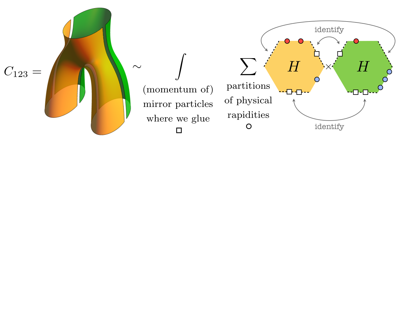
As usual, we depict the three-string interaction/three-point correlator as a pair of pants. Formally, a pair of pants consists of two hexagonal fundamental polygons stitched together at every other side, see figure 1. This, in fact, is how conventional pants are sewed together along their three seams.

In the pair of pants language, each gauge invariant operator corresponds to one of the three circular cuffs and is described by a spin chain or closed string.

When we cut the pair of pants into two hexagons we also cut each closed string into two open strings. Each of these open strings carries some of the excitations of the closed string. Put differently, each of two hexagons is dressed by a subset of the full set of excitations. The contribution to the three-point function for such configuration is then a product of two hexagon form factors as graphically depicted in figure 1. An excitation can end up on either half after cutting and thus we should sum over all such possibilities, see also figure 2.

When we cut the pair of pants into two hexagons we also create three new segments (the pants’ seams) represented by the dashed lines in figure 3. When stitching the hexagons back together we should sum over all possible states living on those dashed lines. This involves integrating over the rapidities of (any number of) mirror excitations.

Altogether we are thus lead to the proposal depicted in figure 1.

More concisely, we are identifying $C_{123}$ with a sort of finite volume two-point function of hexagon operators, each of them associated to the centre of mass of an hexagon. From this point of view the sum over the mirror states is the usual sum arising in form factor studies from inserting the resolution of the identity between the two operators. (This also provides us with a more rigorous motivation for the sum over partitions, see appendix .) This point of view is backed up by a strong coupling world-sheet analysis, as discussed in appendix .

This picture comes along with a notion of asymptotic three-point function, which can be viewed as the natural counterpart of the Beisert-Staudacher asymptotic Bethe ansatz for the spectrum [Beisert:2005fw]. It applies when all lengths involved are large. More precisely, there are two kind of distances in the game: we have the length $L_{i}$ of each external operator and the length $l_{ij}=(L_{i}+L_{j}-L_{k})/2$ ($i,j,k$ all different) of the bridge between two given operators, see figure 3. The latter distances – which are an important novelty of the three-point analysis as compared to the spectrum – control the separation between the two hexagon operators. The asymptotic description applies when these distances are large since then we can project the sum over virtual states to the mirror vacuum. This is nothing but the usual clustering of correlation functions in a gapped theory. In sum, for large bridges (and thus automatically large operators) we can drop the integration over mirror particles and keep the sum over partitions of physical roots only.

At this point, we have reduced the problem of the computation of three-point functions to that of form factors of hexagon operators. The main advantage is that the former can be tackled with a (somehow) conventional integrable bootstrap, reminiscent of the one employed when studying correlators in integrable models [Watson], or branch-point twist fields [Cardy:2007mb]. A similar approach was recently put forward in the context of scattering amplitudes and Wilson loops [Basso:2013vsa].

The most generic hexagon form factor is an intimidating function of six sets of variables. It depends on the physical rapidities of the three operators, as well as on the mirror rapidities of the virtual particles for each of the dashed lines in figure 1. One should add on top of that the six sets of polarizations. We can, however, simplify our life by making use of so-called mirror transformations which map excitations on one edge of the hexagon to a neighbouring one, see figure 4. By sequencially making use of such transformations we can relate any generic hexagon to a much simpler one where all excitations live in a single physical edge. We denote such a creation amplitude as

$${\mathfrak{h}}^{A_{1}\dot{A}_{1},\dots,A_{N}\dot{A}_{N}}(u_{1},\dots,u_{N})\,,$$

(1)

where $A_{i},\dot{A}_{i}$ are $SU(2|2)^{2}$ bifundamental indices parametrizing the polarization of the i-th excitation.

Symmetry-wise the hexagon operator must be singlet under the $PSU(2|2)$ group of symmetries preserved by the three BMN vacua around which we are adding excitations, see appendix . The problem is thus constrained by the very same amount of (super-)symmetries as was Beisert S-matrix [Beisert] or the boundary S-matrix of [DrukkerCorrea] and, as an immediate consequence, its solution is unique, up to an overall scalar factor, for up to two magnons.

Furthermore, combining symmetry arguments with elementary bootstrap considerations hints at a simple and natural generalization to multi-particle states. The conjecture is that the $N$-magnon hexagon amplitude (1) is exactly given by

$${\mathfrak{h}}^{A_{1}\dot{A}_{1}\cdots}\!=\!(-1)^{\mathfrak{f}}\prod_{i<j}{h}_{ij}\langle{\chi}^{\dot{A}_{N}}_{N}\!\!\dots{\chi}^{\dot{A}_{1}}_{1}|\,\mathcal{S}\,|{\chi}^{A_{1}}_{1}\!\!\dots{\chi}^{A_{N}}_{N}\rangle\,,$$

(2)

where ${\chi}^{A}=\phi^{a}|\psi^{\alpha}$ is a state in the fundamental $SU(2|2)$ multiplet and $\mathcal{S}$ is Beisert $SU(2|2)$ S-matrix [Beisert] with dressing phase set to one. ($\mathfrak{f}$ is a simple integer which accommodates for the grading [stat].) The multi-particle formula (2) identifies the hexagon form factor with the (factorized) scattering matrix elements up to the scalar factor $h_{ij}=h(u_{i},u_{j})$, which is a function of two magnon rapidities. The latter can be constrained by crossing symmetry and argued to be given by

$$h_{12}=\frac{x_{1}^{-}-x_{2}^{-}}{x_{1}^{-}-x_{2}^{+}}\frac{1-1/x^{-}_{1}x^{+}_{2}}{1-1/x_{1}^{+}x_{2}^{+}}\frac{1}{\sigma_{12}}\,,$$

(3)

where $x^{\pm}=x(u\pm\frac{i}{2})$ are familiar Zhukowsky variables (with $u/g=x+1/x$) and $\sigma_{12}$ is (half) the BES dressing phase [Beisert:2006ez]. Accordingly, the hexagon form factor is as depicted in figure 5, and its evaluation is straightforward, as exemplified in appendices  and .

It shows, in the end, some similarities with the pentagon transitions for null Wilson loops, in that it factorizes into a dynamical part (the product of $h$’s) and a matrix part (the S-matrix element). An important difference is that the relevant symmetry group for the null Wilson loops was just $SO(6)$ whereas here it involves a more sophisticated supergroup, leading, as a byproduct, to a coupling dependent matrix part.

Relations (2) and (3) finalize our proposal, which provides, in principle, a complete non-perturbative recipe for computing structure constants of any planar gauge invariant operators in this theory. Of course, it is crucial to sharpen it and verify its predictions on the simplest possible examples. This is what the rest of paper is about.

In this section we elaborate on the properties of the hexagon ansatz (2).

An equivalent way of thinking about our problem is by introducing a vertex $\langle\mathfrak{h}|$ which can be contracted against three spin-chain states, like in [Kazama:2014sxa, sbsv, Jiang:2014cya], e.g.

$$\mathfrak{h}^{A\dot{A}}=\langle\mathfrak{h}|\big(|\chi^{A\dot{A}}\rangle_{1}\otimes|0\rangle_{2}\otimes|0\rangle_{3}\big)\,,$$

(4)

for a single magnon on top of the first spin chain. We use here an invariant notation where each operator-ket is thought of as being made out of excitations on top of the same BMN $Z$-vacuum. Implicit in there is the need to actually rotate (and translate) the kets in order to get a non-zero result compatible with $R$-charge conservation. There are several realization of these rotations, one of which is discussed in appendix  and applied (up to a small twist) in the next section.

The symmetry group of each ket in (4) is the usual one for excitations on top of the BMN vacuum, that is the extended $PSU(2|2)^{2}$ introduced by Beisert in [Beisert]. The intersection of the three symmetry groups for the three rotated vacua is a single $PSU(2|2)$, which can be thought of as a diagonal subgroup of symmetries of the BMN vacuum, as explained in appendix . This group is nothing but the supersymmetrization of the obvious bosonic group $O(3)_{\textrm{Lorentz}}\times O(3)_{R-\textrm{charge}}$ that preserves 3 points in space time and 3 (generic) null vectors in ‘$R$-space’.

As mentioned earlier, for low number of magnons, this symmetry leaves very little freedom. For a single magnon, as explained in appendix , it fixes the form factor to be [norm]

$${\mathfrak{h}}^{a\dot{a}}=\langle{\mathfrak{h}}|\Phi^{a\dot{a}}\rangle=\epsilon^{a\dot{a}}\,,\qquad{\mathfrak{h}}^{\alpha\dot{\alpha}}=\langle{\mathfrak{h}}|\mathcal{D}^{\alpha\dot{\alpha}}\rangle={N}\epsilon^{\alpha\dot{\alpha}}\,,$$

(5)

such that the only non-zero one point functions are those corresponding to so-called longitudinal magnons, that is, the two scalars $Y=\Phi^{1\dot{2}},\bar{Y}=\Phi^{2\dot{1}}$ and the two derivatives $D=\mathcal{D}^{1\dot{2}},\bar{D}=\mathcal{D}^{2\dot{1}}$ polarized along the direction of the three-point function. The relative weight ${N}$ is rather arbitrary, since it absorbs the normalization freedom between states of the $PSU(2|2)^{2}\ltimes\mathbb{R}^{3}$ magnon irrep (see e.g. ()). It can be fixed to $N=i$ in the commonly used string frame normalization and to $N=1$ in the spin chain one, see appendix . What is important here is that the one-point function can be seen as a way of contracting the left and right part of a magnon. Put differently, it provides us with an invariant (w.r.t. diagonal $PSU(2|2)$ subgroup) inner product

$$\langle\chi^{\dot{A}}|\chi^{A}\rangle={\mathfrak{h}}^{A\dot{A}}\,,$$

(6)

which is the one implicitly entering in the multi-particle ansatz (2).

As alluded to before, the story repeats at two-particle level where the form factor is fixed to be of the form (2) up to the overall factor $h_{12}$ (see appendix  for details). As an illustration of how this formula works, we can specialize (2) to scalar indices and derive the two-scalar form factor

	$\displaystyle{\mathfrak{h}}^{a\dot{a},b\dot{b}}/h_{12}$	$\displaystyle=\langle\phi^{\dot{b}}_{2}\phi^{\dot{a}}_{1}|\mathcal{S}_{12}|\phi^{a}_{1}\phi^{b}_{2}\rangle$		(7)
		$\displaystyle=A_{12}\langle\phi^{\dot{b}}_{2}|\phi^{\{a}_{2}\rangle\langle\phi^{\dot{a}}_{1}|\phi^{b\}}_{1}\rangle+B_{12}\langle\phi^{\dot{b}}_{2}|\phi^{[a}_{2}\rangle\langle\phi^{\dot{a}}_{1}|\phi^{b]}_{1}\rangle\,,$
		$\displaystyle=A_{12}\epsilon^{a\dot{b}}\epsilon^{b\dot{a}}+\tfrac{1}{2}(A_{12}-B_{12})\epsilon^{ab}\epsilon^{\dot{a}\dot{b}}\,,$

after $\mathcal{S}$-acting as in [Beisert:2006qh] and contracting the resulting bra-ket using (6). We could proceed similarly for derivatives and fermions. In particular, we would find that the form factor ratio between two $Y$’s and two $D$’s is simply given by

$$h_{Y_{1}Y_{2}}/h_{D_{1}D_{2}}=-A_{12}/D_{12}=\frac{x_{1}^{-}-x_{2}^{+}}{x_{1}^{+}-x_{2}^{-}}\,,$$

(8)

upon evaluation of the $A$ and $D$ component of the S-matrix in the spin-chain frame [Beisert, Beisert:2006qh] (with $N=1$). A similar expression can be found in the string frame [reviewHuge, AF-string], as detailed in appendices  and .

Equation (8) illustrates the power of the symmetry. Heuristically, the reason why this symmetry appears so efficient here is that the left and right part of the magnon behave, respectively, as particle and antiparticle w.r.t. the diagonal subgroup (see appendices , and for details). Upon crossing of the right part, the set up becomes thus identical to the one considered by Beisert, which is why its (unique) S-matrix is recovered. The only difference resides in the scalar factor of course, that needs not be unitary in our case.

The ansatz (2) clearly stands as the most natural generalization to many particles, but, as should be clear by now, is not fixed by diagonal $PSU(2|2)$ symmetry alone, for three or more magnons. We shall now provide evidence for it and unveil some of its nice features.

To start with, it is easy to see that the hexagon vertex (2) is automatically preserved by the action of the S-matrix. This is the content of the familiar Watson equation for form factors :

$$\langle{\mathfrak{h}}|(\mathbb{S}_{ii+1}-\mathbb{I})|\ldots\chi^{A_{i}\dot{A}_{i}}_{i}\chi^{A_{i+1}\dot{A}_{i+1}}_{i+1}\ldots\rangle=0\,,$$

(9)

with $\mathbb{S}=S^{0}(-1)^{\dot{F}}\mathcal{S}\,\dot{\mathcal{S}}(-1)^{F}$ the $SU(2|2)^{2}$ S-matrix [trivial]. As depicted in figure 6, this equation immediately follows from the structure of the ansatz and the unitarity of the S-matrix, assuming the scalar factor $h_{12}$ in (2) verifies

$$h_{12}/h_{21}=S_{12}^{0}=\frac{x_{1}^{+}-x_{2}^{-}}{x_{1}^{-}-x_{2}^{+}}\frac{1-1/x^{-}_{1}x_{2}^{+}}{1-1/x^{+}_{1}x^{-}_{2}}\frac{1}{\sigma^{2}_{12}}\,,$$

(10)

where $S_{12}^{0}$ is the spin chain scattering matrix in the $\mathfrak{sl}(2)$ subsector.

A second piece of evidence comes from the so-called decoupling condition. Indeed, form factors typically show kinematical poles whenever a particle-antiparticle pair (with zero net energy and momentum) decouples from the rest of the state. The precise condition can take different form for different type of operators, see e.g. [Watson] for local operators. In our case, it is the form appropriate to the class of non-local operators considered in [Basso:2013vsa, Cardy:2007mb, Basso:2014jfa] that is relevant. Accordingly, we shall insist that our form factors develop a pole, whenever such a pair is formed, with a residue that is simply proportional (i.e. with no interference term) to the form factor for the subprocess in which the pair has been removed. Since our ansatz is directly written in terms of the S-matrix, this condition is easily implemented and almost immediately satisfied. Indeed, on any such a pair, the S-matrix develops a pole with residue mapping to a singlet of the symmetry algebra. This means that we can write

$$\mathcal{S}\big|\chi^{A}_{1}\chi^{B}_{2}\prod_{\textrm{rest}}\chi_{j}\big>_{\textrm{pole}\,(12)}\propto\mathcal{S}_{\textrm{rest}}\prod_{\textrm{rest}}\mathcal{S}_{2j}\mathcal{S}_{1j}\big|\prod_{\textrm{rest}}\chi_{j}\times\mathrm{1}_{21}\rangle$$

(11)

where the equation holds at the level of the pole in the $(12)$ channel and $\big|\mathrm{1}_{21}\big>$ is Beisert singlet [Beisert:2006qh] built out of the particle-antiparticle pair $(12)$. The decoupling is then guaranteed if the scattering between the arbitrary excitation $j$ and the pair $(12)$ is trivial, i.e. equal to $1$, see figure 7. This condition is the same as Janik crossing equation for the S-matrix [Janik:2006dc] as derived by Beisert in [Beisert:2006qh], except that the scalar factor there should now be replaced by $h_{12}$. In other words, for our factorized ansatz, the decoupling condition boils down to the crossing equation

$$h(u_{1}^{2\gamma},u_{2})h(u_{1},u_{2})=\frac{x_{1}^{-}-x_{2}^{-}}{x_{1}^{-}-x_{2}^{+}}\frac{1-1/x^{+}_{1}x_{2}^{-}}{1-1/x^{+}_{1}x_{2}^{+}}\,,$$

(12)

where $u_{1}^{2\gamma}$ denotes the crossed rapidity (corresponding to the swapped Zhukowsky variables $x^{\pm}_{1}\rightarrow 1/x^{\pm}_{1}$).

The simplest solution we could find to both (10) and (12) is the one we reported in (3). [comment]

As mentioned earlier, starting from a form factor with all excitations on the same edge, we can reach any configuration by means of mirror or crossing transformations. These transformations are simpler to implement in the string frame, as explained in detail in appendix . Crossing, in this case, simply amounts to performing twice the analytical continuation $\gamma$ mentioned earlier along with a suitable re-arranging of the indices of the excitations. Precisely, in the string frame,

$$\big|\chi(u^{2\gamma})\big\rangle_{1}\left|0\right>_{2}\left|0\right>_{3}=\left|0\right>_{1}\big|-\tilde{\chi}(u)\big>_{2}\left|0\right>_{3}\,,$$

(13)

with

$$\tilde{\chi}^{A\dot{B}}=\chi^{B\dot{A}}\,,$$

(14)

while, for comparison, in the spin chain frame, one might also have to multiply by extra momentum-dependent factors, as explained in detail in appendix , depending on the excitation. In either frame, the crossing transformation for derivatives is straightforward and simply given by (13), such that e.g. the hexagon process with one $D$ on chain $1$ and its conjugate on chain $2$ reads

$$h_{D|\bar{D}}(u|v)\equiv-h_{DD}(v^{2\gamma},u)\,.$$

(15)

(Explicit expressions for $h_{DD}$ with crossed rapidities are given in appendix .) For identical particles on the two edges, the transition $h_{X|X}(u|v)$ must have a pole at $u=v$ in agreement with (11), see (16) below for details. The residue at this pole is controlled by the measure $\mu_{X}(u)$,

$$\underset{v=u}{\operatorname{{\rm res}}}\,\,h_{X|X}(u|v)=\frac{i}{\mu_{X}(u)}\,.$$

(16)

Recall that in this limit the excitation decouples from the rest, such that the measure just originates from the overlap of the in and out states. It governs the (asymptotic) normalization of the one-particle state and is an essential ingredient for a properly normalized three-point function, as illustrated in section V. A similar measure was introduced in the pentagon approach for null Wilson loops, where it was also used for ‘stapling’ together two pentagons overlapping on a square. The analogous gluing procedure for the hexagons is depicted in figure 9 below.

Let us conclude this section by a brief comment. It so happens that the two hexagons in the three-point function are not absolutely identical. Instead, their form factors differ by $(-1)^{M}$ where $M$ is the total number of magnons. Originally, we found this simple rule by staring at weak and strong coupling data. (It results in the $(-1)^{|\alpha|}$ signs that will pop up everywhere below.) A posteriori, we also came up with a few, plausible but non rigorous, geometrical and kinematical explanations for it. Hopefully, an odd number of such arguments hold. It would be very nice to better understand the origin of this empirical rule, which is responsible for restoring certain symmetries of the structure constants.

The simplest way to access to the elementary hexagon transitions is by considering processes with a single excitation $\chi_{\text{top}}$ with rapidity $u$ on one operator $\mathcal{O}_{1}$ and another single excitation $\chi_{\text{bot}}$ with rapidity $v$ on the operator $\mathcal{O}_{2}$. We shall refer to these operators as top and bottom, respectively, in accord with figure 8. Of course, to probe such simple configurations we have to relax the zero momentum condition for each operator. We shall nevertheless still keep the Bethe ansatz conditions

$$e^{ipL_{1}}=e^{iqL_{2}}=1\,,$$

(17)

where $p=p(u)$ and $q=p(v)$. The third operator $\mathcal{O}_{3}$ has no excitations; it is a BPS operator.

Upon cutting the pants in two, the single excitations on the top or in the bottom can end up on either hexagon. As mentioned above, when an excitation ends on the second hexagon we are instructed to include an extra minus sign. In sum, we expect to find

	$\displaystyle\!\!\!\!\!\!\!\!C_{123}^{\bullet\bullet\circ}$	$\displaystyle\propto$	$\displaystyle h_{\chi_{\text{top}}|\chi_{\text{bot}}}(u|v)+e^{ip\ell_{31}+iq\ell_{12}}h_{\chi_{\text{bot}}|\chi_{\text{top}}}(v|u)$
			$\displaystyle\!\!\!\!\!\!\!\!\!\!-e^{iq\ell_{12}}h_{\chi_{\text{top}}}(u)h_{{\chi}_{\text{bot}}}(v)-e^{ip\ell_{31}}h_{\chi_{\text{top}}}(u)h_{{\chi}_{\text{bot}}}(v)\,.$

All these quantities can be neatly predicted by starting with our finite coupling proposal for the creation amplitude and crossing one of the particles down by a sequence of mirror transformations. For the case of a longitudinal scalar $Y$ and/or its conjugate $\bar{Y}$, for instance, we get

$$h_{Y|Y}=1-\frac{i}{u-v}\,,\,\,\,\,\,h_{Y|\bar{Y}}=-1\,,\,\,\,\,\,h_{Y}=-h_{\bar{Y}}=1\,,$$

(18)

to leading order at weak coupling. We will now compare these predictions against explicit tree level computations.

With this in mind, we introduce a particular realization of the setup above to which we refer as the reservoir picture, see figure 8. In this picture, the first operator $\mathcal{O}_{1}$ is taken to be of the form $\text{Tr\,}(Z\dots Z\chi_{top}Z\dots Z)+\dots$ and is located at $x=0$, the second operator $\mathcal{O}_{2}$ reads $\text{Tr\,}(\bar{Z}\dots\bar{Z}\tilde{\chi}_{bot}\bar{Z}\dots\bar{Z})+\dots$, with $\tilde{\chi}$ as defined in (14), and is located at $x=\infty$ and, finally, the third operator is inserted at $x=(0,1,0,0)$ and reads

$$\mathcal{O}_{3}=\text{Tr\,}(Z+\bar{Z}+Y-\bar{Y})^{L_{3}}\,.$$

(19)

Note that despite the slightly unorthodox appearance, this is a simple (rotated) BPS operator on the same footing as $\text{Tr\,}(Z^{L_{3}})$. The fact that it is rotated (it has to be otherwise one can not properly contract it with the other two in a non-extremal setup) is, however, quite important and justifies the name of the reservoir. We see, for instance, that some excitations of the operators $\mathcal{O}_{1}$ or $\mathcal{O}_{2}$ can be absorbed (i.e. Wick contracted with) by this reservoir. These are precisely the longitudinal excitations introduced earlier. The remaining excitations – namely fermions, transverse derivatives and other scalars – are what we call the transverse excitations. If we insert a transverse excitation in the top (a scalar $X=\Phi^{1\dot{1}}$ say) we ought to introduce its complex conjugate (i.e. $\bar{X}=-\Phi^{2\dot{2}}$) at the bottom or else the result will be zero. In short, the reservoir setup is a realization of the rotations alluded to below (4) and further detailed in appendix , combined with an inversion sending the second operator to infinity.

There are clearly two fundamental quantities arising from the tree-level Wick contractions (see figure 8) in terms of which we can construct any process for different excitations $\chi_{\text{top}}$ and $\chi_{\text{bot}}$. Namely, we can either connect an excitation in the bottom with one at the top by a propagator, thus generating a contribution

$$C^{\text{direct}}=\sum_{n=1}^{\ell_{12}}e^{ip(L_{1}-n+1)+iqn}\,,$$

(20)

or, if the excitation is longitudinal, it can connect directly to the reservoir. When a top/bottom excitation with momentum $p$/$q$ is connected with the reservoir it generates a corresponding contribution of the form

$$C^{\text{reservoir}}_{\text{top}}=\sum_{n=1}^{\ell_{31}}e^{ipn}\,,\,\,\,\,\,\,\,C^{\text{reservoir}}_{\text{bottom}}=\sum_{n=\ell_{12}+1}^{L_{2}}e^{iqn}\,.$$

(21)

It is now a simple matter of appropriately adding up these contributions.

As a warmup, consider a single excitation $Y$ at the top. In this case the structure constant comes from a single term

$$C^{\text{reservoir}}_{\text{top}}=\mathcal{N}(p)(1-e^{ip\ell_{31}})\,,$$

(22)

where $\mathcal{N}(p)=1/(e^{-ip}-1)$ reflects the specific plane wave normalization we are using here. Since this factor plays no role in the following discussion, it will always be implicitly factored out and disregarded. More interesting is the relative minus sign between the two terms in the numerator in (22), which arises trivially from the geometric nature of the series. This is the simplest instance of the minus signs alluded to in the end of the previous section. Apart from this sign and the normalization factor, the result (22) is just the sum of two one point hexagon functions, as expected.

Consider now the more interesting case of a direct transition $Y\to Y$ corresponding to $\chi_{\text{top}}=\chi_{\text{bot}}=Y$. As explained above, in the reservoir picture, this configuration corresponds to inserting a scalar $Y$ at the top and its conjugate $\bar{Y}$ at the bottom (on top of the $Z$ and $\bar{Z}$ vacuum, respectively). These excitations can either be directly connected by a propagator or they can be separately absorbed by the reservoir, see first two pictures in figure 8. The latter contribution ought to pick an additional minus sign w.r.t. the former since in the reservoir operator (19) there is an explicit relative minus sign between the $Y$ and the $\bar{Y}$. Altogether we find therefore

$$\left.C_{123}^{\bullet\bullet\circ}\right|_{Y\to Y}\propto C^{\text{direct}}-C^{\text{reservoir}}_{\text{top}}\times C^{\text{reservoir}}_{\text{bottom}}\,.$$

(23)

Evaluating the simple geometric sums in (20) and (21) and simplifying the outcome using Bethe equations (17) we finally get

	$\displaystyle\left.C_{123}^{\bullet\bullet\circ}\right|_{Y\to Y}$	$\displaystyle\propto$	$\displaystyle(1-\frac{i}{u-v})+e^{ip\ell_{31}+iq\ell_{12}}\times(1-\frac{i}{v-u})$		(24)
			$\displaystyle\!\!\!-e^{iq\ell_{12}}\times 1-e^{ip\ell_{31}}\times 1\,,$

in perfect agreement with our expectations (18). Next, we could look at the transition $Y\to\bar{Y}$ which amounts to inserting a field $Y$ at both the top and bottom. At tree level we cannot contract these fields by a propagator, of course, but they can still be independently absorbed by the reservoir. Accordingly, we must have

$$\left.C_{123}^{\bullet\bullet\circ}\right|_{Y\to\bar{Y}}\propto C^{\text{reservoir}}_{\text{top}}\times C^{\text{reservoir}}_{\text{bottom}}\,,$$

(25)

or equivalently

	$\displaystyle\left.C_{123}^{\bullet\bullet\circ}\right|_{Y\to\bar{Y}}$	$\displaystyle\propto$	$\displaystyle(-1)+e^{ip\ell_{31}+iq\ell_{12}}\times(-1)$		(26)
			$\displaystyle\!\!\!-\,e^{iq\ell_{12}}\times(-1)-e^{ip\ell_{31}}\times(-1)\,,$

which is again in perfect agreement with our expectations (18). Consider finally the case where the scalar is a transverse excitation $X$. Then only the direct propagator contributes and

$$\left.C_{123}^{\bullet\bullet\circ}\right|_{X\to\bar{X}}\propto C^{\text{direct}}\,.$$

(27)

We can therefore simply add up the right hand sides of (24) and (26) to get

	$\displaystyle\left.C_{123}^{\bullet\bullet\circ}\right|_{X\to\bar{X}}$	$\displaystyle\propto$	$\displaystyle-\frac{i}{u-v}+e^{ip\ell_{31}+iq\ell_{12}}\times\frac{-i}{v-u}+$		(28)
			$\displaystyle\!\!\!e^{iq\ell_{12}}\times 0+e^{ip\ell_{31}}\times 0\,.$

From the zeros in the second line, we learn that there is no one point function for such transverse excitations, in line with the symmetry analysis, while from the first line we derive that

$$h_{X|\bar{X}}=-\frac{i}{u-v}\,,$$

(29)

which perfectly matches with what we would extract out of our ansatz.

It is not so much complicated to extend the previous analysis to loop level. It suffices to decorate the tree level Wick contraction by the insertion of the one loop scalar dilatation operator at the splitting points [oneLoopC123]. Using the single excitation case to normalize our three-point function, we can then promptly read off the first quantum correction to various $h$-transitions. In this way we would find

	$\displaystyle h_{Y|Y}(u,v)=\frac{u-v-i}{u-v}\Big[1+\frac{g^{2}}{(u^{2}+\tfrac{1}{4})(v^{2}+\tfrac{1}{4})}+O(g^{4})\Big]\,,$
	$\displaystyle h_{Y|\bar{Y}}(u,v)=-1+O(g^{4})\,,$
	$\displaystyle h_{X|\bar{X}}(u,v)=h_{Y|Y}(u,v)+h_{Y|\bar{Y}}(u,v)\,,$		(30)

in perfect agreement with the one loop expansion of our all loop conjectures. Note in particular that the function $h_{Y|Y}(u,v)$ is nothing but the loop corrected $f(v,u)$ in [tailoring4].

We further extended the tree level analysis above to all other magnon excitations always finding a perfect match with our predictions. (See also appendices , and for more involved checks at weak coupling.) For fermions, for instance, we could use the recent results for the splitting insertions of [ThiagoJoao] to test their transition up to one loop. In the end, it is quite amusing that so much of the full result can already be checked with such simple computations involving no more than one particle in the top and another in the bottom!

Putting together all the ingredients in our main proposal we will now write down the final prediction for the asymptotic all-loop structure constants for some simple (so-called rank one) sectors involving one non-trivial operator and two protected operators. Our proposal will extend the one loop results of [tailoring1, tailoring4] and [tailoringNC] – for $SU(2)$ and $SL(2)$ correlators respectively – to all loops. Both can be described at once, by replacing $h$ below by $h_{DD}$ for the $SL(2)$ case or by $h_{YY}$ for the $SU(2)$ setup, and similarly for all other dynamical quantities. To avoid unimportant combinatorial normalization factors we present here the ratio between the structure constant and a structure constant of three BPS operators with the same lengths. Our conjecture then concisely reads

$$\left(\frac{C_{123}^{\bullet\circ\circ}}{C_{123}^{\circ\circ\circ}}\right)^{2}=\frac{\prod_{k=1}^{S}\mu(u_{k})}{\det\,\partial_{u_{i}}\phi_{j}\prod_{i<j}S(u_{i},u_{j})}\times\mathcal{A}^{2}\,,$$

(31)

where $S$ is the number of magnons in the non-protected operator (scalars $Y$ in the $SU(2)$ case or derivatives $D$ for the $SL(2)$ setup). It makes use of the measure $\mu(u)$ defined through the residue of the direct transition as in (16), of the Gaudin norm (here in rapidity $u$ and not momentum $p$ space) defined with

$$e^{i\phi_{j}}\equiv e^{ip_{j}L_{1}}\prod_{k\neq j}S(u_{j},u_{k})\,,$$

(32)

and of a product of scattering phases. So combined, these quantities permit the conversion between infinite- and finite-volume normalizations, see e.g. [Pozsgay:2009pv, Bajnok:2015hla] and references therein for relativistic systems.

Finally, and most interestingly, we have the sum over the hexagon processes, which can be cast into the form

$$\mathcal{A}=\prod_{i<j}h(u_{i},u_{j})\sum_{\alpha\cup\bar{\alpha}={\bf u}}(-1)^{|\bar{\alpha}|}\prod_{j\in\bar{\alpha}}e^{ip_{j}\ell}\prod_{i\in\alpha,j\in\bar{\alpha}}f(u_{i},u_{j})$$

(33)

where we sum over all bipartite partitions $\alpha\cup\bar{\alpha}=\{u_{i}\}$ of the set of Bethe rapidities, with $f(u,v)=1/h(u,v)$ and with the splitting length $\ell=\ell_{31}$. A few more comments on this expression and on the connection to previous expressions in the literature for such correlators at low loop order are presented in appendix .

The asymptotic formula (31) for $C_{123}^{\bullet\circ\circ}$ can be systematically improved by incorporating finite-size corrections. In our picture, these ones come about when particles get exchanged between the two hexagons. At weak coupling, the heavier the exchanged state is the later it contributes in perturbation theory. The leading finite-size corrections are thus obtained when a single particle is passing through one of the three mirror channels along which we glue the two hexagons together, see figure 9. This amounts to replacing $\mathcal{A}$ in (31) by

$$\mathcal{A}\to\mathcal{A}+\delta\mathcal{A}_{{12}}+\delta\mathcal{A}_{{23}}+\delta\mathcal{A}_{{31}}\,,$$

(34)

where the corrections $\delta\mathcal{A}_{{12}}$ and $\delta\mathcal{A}_{{31}}$ are associated to the neighboring bridges while $\delta\mathcal{A}_{{23}}$ is the contribution from the opposing bridge. As we will see they yield very different contributions. Nevertheless, regardless of which one of these channels we consider, the one-particle contribution always takes the form

$$\delta\mathcal{A}=\sum_{a\geqslant 1}\int\frac{du}{2\pi}\mu^{\gamma}_{a}(u)\times\left(\frac{1}{x^{[+a]}x^{[-a]}}\right)^{\ell}\times\textrm{int}_{a}(u|\{u_{i}\})\,,$$

(35)

with $\ell$ the size of the corresponding bridge. The recipe is that we ought to sum over the tower of bound states ($a=1,2,...$) and integrate over the rapidity $u$ of the mirror excitation with the help of the mirror measure $\mu^{\gamma}_{a}(u)\equiv\mu_{a}(u^{\gamma})$. For a bound state of $a$ derivatives, this measure reads explicitly as [fusion]

$$\mu_{a}(u^{\gamma})=\frac{a(x^{[+a]}x^{[-a]})^{2}}{g^{2}(x^{[+a]}x^{[-a]}-1)^{2}((x^{[+a]})^{2}-1)((x^{[-a]})^{2}-1)}\,,$$

(36)

with $x^{[\pm a]}=x(u\pm i\frac{a}{2})$, and it differs by an overall sign from the mirror measure for the bottom (or $Y$-like) component in the same supermultiplet. Thanks to the diagonal $O(3)\times O(3)$ symmetry, these are the only cases we have to consider; that is, for the type of three-point functions under study, the mirror excitation in (35) can only be one of the longitudinal bosons $D,\bar{D},Y,\bar{Y}$ or one of their homologues in the bound state multiplet. For sake of clarity, the corresponding flavour summation is implicitly understood in (35) and subsumed into the integrand $\textrm{int}_{a}$ as explained below.

The second term in the integrand in (35) is the usual damping factor $e^{-\ell E_{a}(u)}$ which accommodates for the propagation through a distance $\ell$ of a mirror particle with energy $E_{a}=\log{x^{[+a]}x^{[-a]}}$.

Finally, the last remaining ingredient is the integrand $\textrm{int}_{a}(u|\{u_{i}\})$ which collects the hexagon form factors for creation and annihilation of the mirror excitation in the background of real magnons $\{u_{i}\}$.

Based on this data alone, we can already estimate the finite size correction at weak coupling. Since in this limit $x^{[\pm a]}\sim(u\pm ia/2)/g$, the integral (35) is found to be parametrically of order $O(g^{2+2\ell})$, assuming an integrand $\textrm{int}_{a}(u|\{u_{i}\})$ of order $O(1)$. The virtual effects captured by (35) thus start generically at $(\ell+1)$ loops for a bridge of size $\ell$, which means, in particular, two loops for the smallest (non-extremal) bridge, with $\ell=1$.

The integral (35) mimics in many ways the Lüsher formula for the spectrum [Bajnok:2008qj]. In fact, the parallelism goes even further since its integrand also features a transfer matrix. To see that, we need to look more closely at what is running inside the integrand. For the sake of clarity, we shall consider the $a=1$ contribution to the adjacent mirror channel (obtained by a single $\gamma$ move away from the excited cuff of the pants). In this case, we get

$\displaystyle\textrm{int}^{\gamma}(u|\{u_{i}\})=\sum_{\alpha\cup\bar{\alpha}=\{u_{i}\}}w(\alpha,\bar{\alpha})(-1)^{|\alpha|}\times$

(37)