Newtonian wormholes with spherical symmetry and tidal forces on test particles

Our purpose is to make use of Eqs. (1)-(3) to construct a static, spherical symmetric wormhole space. Let us then generically write the metric of the space as

$$ds^{2}=A\left(r\right)dr^{2}+r^{2}\left(d\theta^{2}+\sin^{2}\theta\,d\varphi^{2}\right)\,,$$

(5)

such that the Ricci scalar $R$ is

$$R=\frac{2\left[\left(A\left(r\right)-1\right)A\left(r\right)+rA^{\prime}\left(r\right)\right]}{r^{2}A\left(r\right){}^{2}}\,.$$

(6)

Now, to proceed we consider the expression for the mass density to be

$$\rho\left(r\right)=\alpha e^{-\frac{r^{2}}{b^{2}}}\left(2-\frac{b^{2}}{r^{2}}\right)\,,$$

(7)

where $\alpha$ has dimensions of mass density and $b$ of distance. Substituting Eqs. (6) and (7) in Eq. (3) we find the general form of the metric, for the imposed mass density,

$$ds^{2}=\frac{r}{r+\beta\,re^{-\frac{r^{2}}{b^{2}}}+C_{1}}\,dr^{2}+r^{2}\left(d\theta^{2}+\sin^{2}\theta\,d\varphi^{2}\right)\,,$$

(8)

where $C_{1}$ is an integration constant and

$$\beta\equiv b^{2}k\alpha\,.$$

(9)

Having found the generic form of the metric, we have now to restrict the values of the parameters $C_{1}$, $\alpha$ and $k$ to have a wormhole geometry. For such, we will follow [6] and use an embedding diagram. So, in the Euclidean embedding space the axially symmetric embedded surface can be, using cylindrical coordinates $(\bar{r},z,\bar{\varphi})$, uniquely described by a function $z(r)$. Identifying the coordinates $\left(\bar{r},\bar{\varphi}\right)$ of the embedding Euclidean space with the coordinates $\left(r,\varphi\right)$ of the wormhole space, we find the following relation

$$\frac{dz}{dr}=\pm\sqrt{\frac{r}{r+\beta\,re^{-\frac{r^{2}}{b^{2}}}+C_{1}}-1}\,,$$

(10)

which can be used to study the properties of the space. From Eq. (10) and imposing the throat condition we find that the integration constant $C_{1}$ is given by

$$C_{1}=-b\left(1+\frac{\beta}{e}\right)\,,$$

(11)

and the range of values of the parameter $\beta\equiv k\alpha\,b^{2}$ is constrained to be $-\infty<\beta<e$. The same restriction to the parameter $\beta$ is found from the flare-out condition. Substituting Eq. (11) in Eq. (8) we find

$$ds^{2}=\frac{1}{1-\frac{b(r)}{r}}dr^{2}+r^{2}\left(d\theta^{2}+\sin^{2}\theta d\varphi^{2}\right)\,,$$

(12)

where

$$b\left(r\right)=b+\frac{\beta}{e}\left(b-re^{1-\frac{r^{2}}{b^{2}}}\right)\,.$$

(13)

Another restriction to have a wormhole geometry is that although near the wormhole’s throat, $r=b$, the radial coordinate $r$ is ill behaved, the proper radial distance must be finite. This condition implies a new restriction to $\beta$

$$-\infty<\beta\leqslant\beta_{{\rm crit}}\,,$$

(14)

where the critical value of $\beta$ is given by $\beta_{{\rm crit}}\equiv\inf_{1\,\leq\,\frac{r}{b}\,<\,\infty}\left[\frac{\frac{r}{b}-1}{e^{-1}-\frac{r}{b}\,e^{-\frac{r^{2}}{b^{2}}}}\right]$, and $\inf$ represents the infimum of the function in the specified range. This gives

$$\beta_{\rm crit}=2.338\,,$$

(15)

up to the third decimal place. Comparing Eq. (15) with the restriction found from the throat condition, $\beta<e$, we conclude that the product $\beta=k\alpha\,b^{2}$ is then restricted by Eqs. (14) and (15).

Due to the range of values that the parameter $\beta$ might take, various distinct cases could be considered. Here we shall be interested in the class of wormholes whose parameters $\alpha$, $k$ and $b$ obey $0<\beta\leqslant\beta_{{\rm crit}}$ together with $\alpha>0$, and so $k>0$.

Now we use Eq. (4) to study the motion of a test particle in the gravitational field of the wormhole space. Consider that a particle’s path is described by a curve $\gamma$, whose components $x^{i}$ are given by $x^{i}=\left(l\left(t\right),\theta\left(t\right),\varphi\left(t\right)\right)$ such that the particle’s velocity is $v^{i}\equiv\dot{x}^{i}$, where a dot means a derivative with respect to time $t$. The right hand side of Eq. (4) is the gravitational field given in Eq. (19) and the left hand side the acceleration of the particle, defined as $a^{i}=v^{j}\,\nabla_{j}\,v^{i}$. It is possible to show that one can treat the problem of the motion of a test particle by considering pure equatorial orbits, i.e., $\theta=\frac{\pi}{2}$, $\dot{\theta}=0$ and $\ddot{\theta}=0$. Gathering these results the equations of motion are

	$\displaystyle\ddot{l}+\left[\frac{b\,e^{\frac{l^{2}}{b^{2}}}\left(2b^{2}+l^{2}\right)\left(e+\beta\right)-2\sqrt{b^{2}+l^{2}}\left[\beta\,l^{2}\left(1+l^{2}/b^{2}\right)+b^{2}\left(e^{1+\frac{l^{2}}{b^{2}}}+\beta\right)\right]}{2l\left(b^{2}+l^{2}\right)\left[b\,e^{\frac{l^{2}}{b^{2}}}\left(e+\beta\right)-\sqrt{b^{2}+l^{2}}\left(e^{1+\frac{l^{2}}{b^{2}}}+\beta\right)\right]}\right]\,\,\dot{l}{}^{2}+$		(22)
	$\displaystyle\hskip 70.2625pt+\left[\frac{b\sqrt{b^{2}+l^{2}}\left(e+\beta\right)-\left(b^{2}+l^{2}\right)\left(e+\beta\,e^{-\frac{l^{2}}{b^{2}}}\right)}{e\,l}\right]\,\,\dot{\varphi}{}^{2}=$
	$\displaystyle\hskip 70.2625pt=-\frac{G\,m\left(l\right)}{2\sqrt{e}\,\left(b^{2}+l^{2}\right)l}\sqrt{\left(b^{2}+l^{2}\right)\left(e+\beta\,e^{-\frac{l^{2}}{b^{2}}}\right)-b\sqrt{b^{2}+l^{2}}\left(e+\beta\right)}\,,$

$$\theta=\frac{\pi}{2}\,,\quad\dot{\theta}=0\,,$$

(23)

$$\ddot{\varphi}+2\,\frac{l}{b^{2}+l^{2}}\,\,\dot{l}\,\dot{\varphi}=0\,.$$

(24)

Having found the equations of motion of a test particle, we have now to solve them. Let us consider the simpler problem of a test particle describing pure circular motion in the Newtonian wormhole space. In this case the coordinate $l$ is a constant, $l_{0}$, say, so $\dot{l}=0$ and $\ddot{l}=0$. From this, Eq. (22) can be solved for $\dot{\varphi}$ and obtain

$$\dot{\varphi}=\sqrt{\frac{\sqrt{e}\,G\,m\left(l_{0}\right)}{2\left(b^{2}+l_{0}^{2}\right)\sqrt{\left(b^{2}+l_{0}^{2}\right)\left(e+\beta\,e^{-\frac{l_{0}^{2}}{b^{2}}}\right)-b\sqrt{b^{2}+l_{0}^{2}}\left(e+\beta\right)}}}\,.$$

(25)

Eq. (25) relates the radial position $l_{0}$ and the angular velocity $\dot{\varphi}$ for a particle to describe a circular orbit in the wormhole space. Now, except the case of pure circular motion, to solve the equations of motion (22)-(24) for a more generic motion, numerical methods must be used, provided the initial position and velocity of the test particle and the wormhole parameters $b$ and $\alpha$ are given.

We now analyze the relative separation of two test particles in the gravitational field of the spherical Newtonian wormhole space. The two test particles are initially considered to be infinitesimally close, subjected only to the gravitational field of the Newtonian wormhole, such that the acceleration of a test particle at a certain point is given by Eq. (4) and Eqs. (19)-(20). This relative separation, i.e., the tidal deviation equation, is in part given by the variation of the gravitational force field acted on each particle and another part given by the geodesic deviation due to the spatial curvature through the equation,

$$\frac{D^{2}n^{i}}{dt^{2}}=n^{k}\left(-\nabla_{k}\mathcal{G}^{i}+R_{jlk}^{i}v^{j}v^{l}\right)\,,$$

(26)

where $n^{i}$ is the separation vector between two infinitesimally close particles, $\mathcal{G}^{i}$ is the gravitational force field generated by the wormhole mass, given by Eq. (19), $v^{i}$ is the velocity of the fiducial test particle and $R_{jlk}^{i}$ represents the Riemann tensor.

Let us simplify the calculations, by remarking that, as was mentioned in Sec. (3.3), the velocity of the fiducial test particle can be assumed to be along the equator, $\theta=\pi/2$ (see Eq. (23)). Hence, in Eq. (26), we might take all the terms in $v^{\theta}$ to zero. Notice, however, that this does not mean that, in general, the acceleration of the component $n^{\theta}$ of the separation vector is zero since the motion of the second particle may not be along the equator. Now, considering the metric of the spherical Newtonian wormhole space, Eq. (16), and assuming $\theta=\pi/2$ and $\dot{\theta}=0$, we find from Eq. (26) that the deviation equations for two infinitesimally close test particles in the spherically symmetric Newtonian wormhole space are

	$\displaystyle\frac{D^{2}n^{l}}{dt^{2}}=$	$\displaystyle-n^{l}\left(\partial_{l}\mathcal{G}^{l}+\Gamma_{ll}^{l}\mathcal{G}^{l}\right)+R_{\varphi l\varphi}^{l}v^{\varphi}\left(n^{\varphi}v^{l}-n^{l}v^{\varphi}\right)\,,$			(27)
	$\displaystyle\frac{D^{2}n^{\theta}}{dt^{2}}=$	$\displaystyle n^{\theta}\left[-\Gamma_{\theta l}^{\theta}\mathcal{G}^{l}+R_{ll\theta}^{\theta}\left(v^{l}\right)^{2}+R_{\varphi\varphi\theta}^{\theta}\left(v^{\varphi}\right)^{2}\right]\,,$			(28)
	$\displaystyle\frac{D^{2}n^{\varphi}}{dt^{2}}=$	$\displaystyle-\Gamma_{\varphi l}^{\varphi}\mathcal{G}^{l}n^{\varphi}+R_{ll\varphi}^{\varphi}v^{l}\left[n^{\varphi}v^{l}-n^{l}v^{\varphi}\right]\,.$			(29)

where the Christoffel symbols that appear in Eqs. (27)-(29) have the form

$$\Gamma_{ll}^{l}=\frac{b^{3}(\beta+e)e^{\frac{l^{2}}{b^{2}}}\left(2b^{2}+l^{2}\right)-2\sqrt{b^{2}+l^{2}}\left[l^{2}\beta\left(b^{2}+l^{2}\right)+b^{4}\left(e^{\frac{l^{2}}{b^{2}}+1}+\beta\right)\right]}{2b^{2}l\left(b^{2}+l^{2}\right)\left[b(\beta+e)e^{\frac{l^{2}}{b^{2}}}-\sqrt{b^{2}+l^{2}}\left(e^{\frac{l^{2}}{b^{2}}+1}+\beta\right)\right]}\,,$$

(30)

$$\Gamma_{\theta l}^{\theta}=\Gamma_{\varphi l}^{\varphi}=\frac{l}{b^{2}+l^{2}}\,.$$

(31)

The other non-zero Christoffel symbols necessary to calculate the Riemann tensor components are $\Gamma_{\varphi\varphi}^{l}=\Gamma_{\theta\theta}^{l}\sin^{2}\theta$, $\Gamma_{\varphi\theta}^{\varphi}=\cot\theta$, and $\Gamma_{\varphi\varphi}^{\theta}=-\Gamma_{\varphi\theta}^{\varphi}\sin^{2}\theta$. At the plane $\theta=\pi/2$ one has

$$\Gamma_{\theta\theta}^{l}=\Gamma_{\varphi\varphi}^{l}=-\frac{\left(b^{2}+l^{2}\right)\left(\beta e^{-\frac{l^{2}}{b^{2}}}+e\right)-b(\beta+e)\sqrt{b^{2}+l^{2}}}{el}\,,$$

(32)

and $\Gamma_{\varphi\theta}^{\varphi}=\Gamma_{\varphi\varphi}^{\theta}=0$, the remaining Christoffel symbols being zero or given by symmetry of the ones just calculated. The Riemann tensor components appearing in Eqs. (27)-(29), assuming $\theta=\pi/2$, are

	$\displaystyle R_{\varphi l\varphi}^{l}=$	$\displaystyle\frac{2\beta e^{-\frac{l^{2}}{b^{2}}}\sqrt{\left(b^{2}+l^{2}\right)^{3}}-b^{3}(\beta+e)}{2eb^{2}\sqrt{b^{2}+l^{2}}}\,,$			(33)
	$\displaystyle R_{ll\theta}^{\theta}=R_{ll\varphi}^{\varphi}=$	$\displaystyle\frac{l^{2}\left(2\beta\sqrt{\left(b^{2}+l^{2}\right)^{3}}-b^{3}(\beta+e)e^{\frac{l^{2}}{b^{2}}}\right)}{2b^{2}\left(b^{2}+l^{2}\right)^{2}\left(b(\beta+e)e^{\frac{l^{2}}{b^{2}}}-\sqrt{b^{2}+l^{2}}\left(e^{\frac{l^{2}}{b^{2}}+1}+\beta\right)\right)}\,,$			(34)
	$\displaystyle R_{\varphi\varphi\theta}^{\theta}=$	$\displaystyle\frac{\beta e^{-\frac{l^{2}}{b^{2}}}\sqrt{b^{2}+l^{2}}-b(\beta+e)}{e\sqrt{b^{2}+l^{2}}}\,.$			(35)

These equation complete the geodesic deviation equations (27)-(29).

Now, looking at Eqs. (27)-(29), in general, it is not possible to find analytical solutions since the fiducial test particle’s velocity must also be taken into account. So, to solve this system of differential equations, we must first solve the equations of motion, Eqs. (22)-(24), and in general there is no analytical solution. We can however work out some features of the tidal effects in the case of pure radial motion of two test particles such that throughout the motion the line that connects the two particles is purely radial, i.e., the case where $n^{\theta}$, $n^{\varphi}$, $v^{\theta}$, and $v^{\varphi}$ are zero throughout the particles’ motion. In this case Eq. (27) simplifies to

$$\frac{D^{2}n^{l}}{dt^{2}}=-n^{l}\left(\partial_{l}\mathcal{G}^{l}+\Gamma_{ll}^{l}\mathcal{G}^{l}\right)\,,$$

(36)

and Eqs. (28) and (29) yield $\frac{D^{2}n^{\theta}}{dt^{2}}=0$ and $\frac{D^{2}n^{\varphi}}{dt^{2}}=0$, respectively. Although it is still not possible to solve analytically Eq. (36) we can instead make a qualitative analysis to infer the general behavior of two initially close test particles describing pure radial motion.

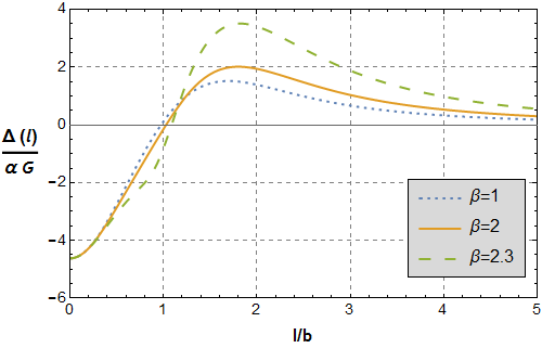
Defining the right hand side of Eq. (36) as

$$\Delta\left(l\right)\equiv-\partial_{l}\mathcal{G}^{l}-\Gamma_{ll}^{l}\mathcal{G}^{l}$$

(37)

we present in Fig. 2 its behavior. We see that the sign of the function $\Delta$ changes at some value of the coordinate $l$, $l_{c}$, say. Now, when $l>l_{c}$ the function $\Delta\left(l\right)$ is positive, $\Delta\left(l\right)>0$, which implies that the separation vector has positive acceleration. So, suppose two test particles describing pure radial motion, such that the line that connects them is purely radial. One particle has radial coordinate $l_{1}$, the other $l_{2}$, and let us assume, $l_{1}<l_{2}$ and $l_{1,2}>l_{c}$ with $l_{c}>0$ for simplicity. In this case, since $\Delta\left(l\right)>0$, the particle with coordinate $l_{1}$ is accelerating more than the particle with coordinate $l_{2}$, and they fly apart. On the other hand, for $l<l_{c}$ the function $\Delta\left(l\right)$ is negative, $\Delta\left(l\right)<0$, so the separation vector has negative acceleration. Assuming now $l_{1,2}<l_{c}$, and still $l_{1}<l_{2}$, this means that the particle with coordinate $l_{1}$ is accelerating less, but still towards the wormhole’s throat, than the particle with coordinate $l_{2}$. Numerically solving Eq. (36) for two initially close test particles in the regions $l>l_{c}$ and $l<l_{c}$, indeed, we verify this conclusions. Notice that as we consider particles further away from the wormhole’s throat we recover the tidal behavior expected from Newtonian gravitation since the space is asymptotically flat.

References

- [1] M. Abramowicz, “The perihelion of Mercury advance calculated in Newton’s theory”, arXiv:1212.0264 [astro-ph.EP] (2012).
- [2] M. Abramowicz, G. F. R. Ellis, J. Horák, and M. Wielgus, “The perihelion of Mercury advance and the light bending calculated in (enhanced) Newton’s theory”, Gen. Relativ. Gravit 46, 1630 (2014); arXiv:1303.5453 [gr-qc] (2013).
- [3] J. Ehlers, “Contributions to the relativistic mechanics of continuous media”, Gen. Relativ. Gravit 25, 1225 (1993), (translation of the Proceedings of the Mathematical-Natural Science Section of the Mainz Academy of Science and Literature 11, 792 (1961)).
- [4] G. F. R. Ellis and H. van Elst, “Cosmological models”, in Proceedings of the NATO Advanced Study Institute on Theoretical and Observational Cosmology, Cargèse, NATO Science Series, Series C, Mathematical and Physical Sciences 541, 1, ed. M. Lachièze-Rey (Kluwer Academic, Boston 1999); arXiv:gr-qc/9812046.
- [5] J. P. S. Lemos and P. Luz, “Newtonian wormholes”, Gen. Rel. Grav. 46 1803 (2014); arXiv:1409.3231 [gr-qc].
- [6] M. S. Morris, and K. S. Thorne, “Wormholes in spacetime and their use for interstellar travel: A tool for teaching general relativity”, Am. J. Phys. 56, 395 (1988).
- [7] M. Visser, Lorentzian wormholes: From Einstein to Hawking (AIP Press, American Institute of Physics, 1995).
- [8] J. P. S. Lemos, F. S. N. Lobo, and S. Q. Oliveira, “Morris-Thorne wormholes with a cosmological constant”, Phys. Rev. D 68, 064004 (2003); arXiv:gr-qc/0302049.
- [9] A. B. Balakin, J. P. S. Lemos, and A. E. Zayats, “Nonminimal coupling for the gravitational and electromagnetic fields: Traversable electric wormholes”, Phys. Rev. D 81, 084015 (2010); arXiv:1003.4584 [gr-qc].
- [10] G. A. S. Dias and J. P. S. Lemos, “Thin-shell wormholes in d-dimensional general relativity: Solutions, properties, and stability”, Phys. Rev. D 82, 084023 (2010); arXiv:1008.3376 [gr-qc].