Pivoted Cholesky decomposition by cross approximation for efficient solution of kernel systems

Interpolation of spatial data with kernel functions [27] finds wide application in many fields of scientific computing. The system of equations is prone to be ill-conditioned when a large number of data or smooth kernel functions are used in hope of improving accuracy. Nevertheless a good interpolation accuracy is usually accompanied by a large condition number of the interpolation matrix [26]. This is like a high-wire walk between two abysses, bad accuracy on the left and numerical instability on the right, no wonder various regularization techniques [23] are usually adopted as safety ropes. In this paper we show pivoted Cholesky decomposition, a matrix approximation technique, is an efficient solver in this situation which guarantees the stability without the perturbation of regularization while reduces the complexity of solution from $\mathcal{O}(n^{3})$ to $\mathcal{O}(k^{2}n)$ for a rank-$k$ system. We propose an improved pivoted Cholesky decomposition algorithm by tuning cross approximation technique to symmetric and positive definite matrices.

Pivoted Cholesky decomposition (PCD)[8, 11, 16, 17] and cross approximation [4, 5] are two favourable low rank approximation techniques with linear complexity in $n$ (in contrast to the cubic complexity of a truncated singular value decomposition). Compared to other techniques of linear complexity like the Nyström approximation [31, 9] and sparse greedy approximations [29] they are more accurate due to the pivot maximizations [1]. Another advantage is that they provide deterministic error bounds and thus can be run adaptively to a certain accuracy.

PCD is a pivoted version of the outer product Cholesky algorithm [12, Algorithm 4.2.2] that chooses the diagonal entry with the largest modulus as the pivot. In each step a rank-1 approximation is made based on the column and row cross at the pivot so that $k$ steps accumulate a rank-$k$ approximation. Earlier versions of this algorithm, e.g. LINPACK routine SCHDC [8], include a global updating in which the rank-1 approximation is subtracted from the remainder matrix (or the original matrix for the first step), this made them more expensive than the later ones in [11, 2, 3, 16, 17]¹¹ 1 In [2, 3] this method was introduced by the name of incomplete Cholesky decomposition in which the updating only occurs in the pivoted columns.

When cross approximation (CA) is applied to symmetric positive definite matrices it produces similar results as a PCD, i.e. the results are only a row permutation away from triangular matrices. If the pivot is chosen only on the diagonal, the fully pivoted CA and the early version of PCD are nearly identical with the only difference in the permutation. Such a CA was proposed in [25] to produce a diagonalised decomposition. While choosing the pivot on the diagonal in PCD is justified in [3] as maximising the lower bound of gain in each step, it is not yet fully justified in the language of CA. The CA algorithm, with the merit of being simpler (without row swapping and nested entry indexing) and providing sharp error bound in uniform norm, can be adapted to a PCD if this gap is bridged.

In this work we first bridge this gap and merge the merits of the two regimes into a new PCD algorithm which is simpler and gives sharp uniform-norm error bound, and then justify the validity and efficiency advantage of the algorithm in solving ill-conditioned kernel systems.

The rest of this paper is organized as follows. In Section 2 we recall the basic Cross Approximation algorithm and introduce an adaption to symmetric positive definite matrices. In Section 3 we extend the adapted CA to PCD. In Section 4 we justify the PCD solution to rank deficient kernel systems. Section 5 gives applications of the algorithms. Section 6 summarizes the whole paper.

Cross approximation (CA) is an iterative matrix approximation technique [4, 5] that yields a factorization equivalent to a skeleton decomposition [4, Lemma 3]. Like in many other methods, CA constructs a rank-$k$ approximation by using only a small portion, i.e. some $k$ rows and $k$ columns, of the matrix. Hence it is widely used for data compression [21, 10]. It is justified in [13] that the columns and rows should be such chosen that their intersection has the largest determinant in modulus among all $k\times k$ submatrices (the maximal-volume principle), and it is shown in [14] that such an approximation is quasi-optimal in the uniform norm.

In each step of CA, a rank-1 approximation is made and subtracted from the remainder matrix. It turns out that choosing the pivot (the intersection of the chosen column and row that form the rank-1 approximation) as the entry with the largest modulus in the remainder matrix is the optimal strategy in term of maximal-volume principle if we keep the pivot points in the previous steps fixed (like in CA) [4, Lemma 2] .

For very large matrices, CA with global pivot searching and global updating (which is termed as fully pivoted CA) is expensive or even prohibitive. A trade-off of accuracy and cost is made in the so-called partially pivoted CA which only searches for the pivot in some chosen rows and columns.

However, if the underlying matrix is symmetric positive semi-definite (SPSD) much of the cost of a fully pivoted CA can be saved without sacrificing accuracy. This is due to the fact that the diagonal entries of SPSD matrices always include the maximum in modulus, and that the remainder matrices can be kept SPSD during the CA steps.

A SPSD matrix-adapted CA is proposed in this section. This algorithm has a complexity linear in the matrix size as does the partially pivoted CA, while retains the accuracy of a fully pivoted CA. We start by introducing the “baseline” — the fully pivoted CA algorithm.

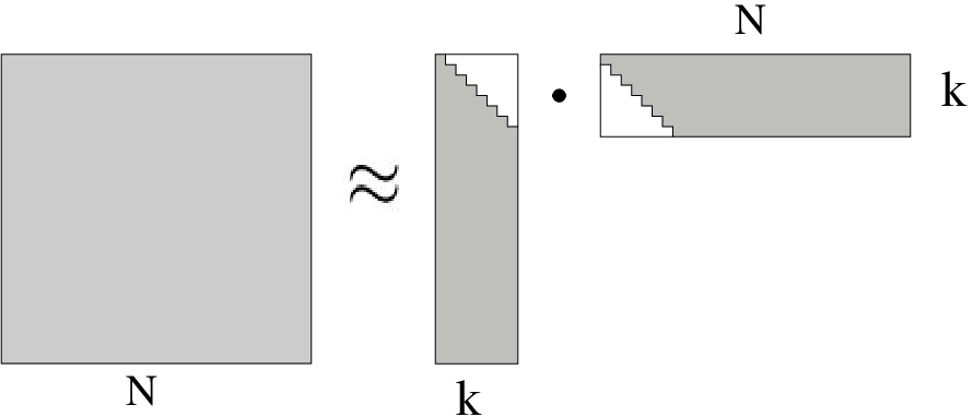
In Equation (3) we see that in each step the CA algorithm leaves one additional zero column and zero row in the remainder matrix, so that the $j$-th column of $\mathchoice{\displaystyle\mathbf{A}}{\textstyle\mathbf{A}}{\scriptstyle\mathbf{A}}{\scriptscriptstyle\mathbf{A}}$ has one more zero entry than the $(j-1)$-th, hence $\mathchoice{\displaystyle\mathbf{A}}{\textstyle\mathbf{A}}{\scriptstyle\mathbf{A}}{\scriptscriptstyle\mathbf{A}}$ is just a row permutation away from a triangular matrix. Appending a row permutation to Algorithm 2 leads to a pivoted Cholesky decomposition, $\widetilde{\mathchoice{\displaystyle\mathbf{M}}{\textstyle\mathbf{M}}{\scriptstyle\mathbf{M}}{\scriptscriptstyle\mathbf{M}}}\approx\mathchoice{\displaystyle\boldsymbol{L}}{\textstyle\boldsymbol{L}}{\scriptstyle\boldsymbol{L}}{\scriptscriptstyle\boldsymbol{L}}\mathchoice{\displaystyle\boldsymbol{L}}{\textstyle\boldsymbol{L}}{\scriptstyle\boldsymbol{L}}{\scriptscriptstyle\boldsymbol{L}}^{\top}$ with $\mathchoice{\displaystyle\boldsymbol{L}}{\textstyle\boldsymbol{L}}{\scriptstyle\boldsymbol{L}}{\scriptscriptstyle\boldsymbol{L}}$ a $n$-by-$k$ lower triangular matrix and $\widetilde{\mathchoice{\displaystyle\mathbf{M}}{\textstyle\mathbf{M}}{\scriptstyle\mathbf{M}}{\scriptscriptstyle\mathbf{M}}}$ a symmetric permutation of $\mathchoice{\displaystyle\mathbf{M}}{\textstyle\mathbf{M}}{\scriptstyle\mathbf{M}}{\scriptscriptstyle\mathbf{M}}$ based on an index $\mathchoice{\displaystyle\boldsymbol{p}}{\textstyle\boldsymbol{p}}{\scriptstyle\boldsymbol{p}}{\scriptscriptstyle\boldsymbol{p}}$ yielded by the algorithm, as detailed in Algorithm 3 and diagrammed in the upper part of Figure 1. The algorithm also produces a $k$-by-$k$ triangular matrix $\mathchoice{\displaystyle\boldsymbol{L}}{\textstyle\boldsymbol{L}}{\scriptstyle\boldsymbol{L}}{\scriptscriptstyle\boldsymbol{L}}_{*}$ that exactly reproduces the submatrix $\mathchoice{\displaystyle\mathbf{M}}{\textstyle\mathbf{M}}{\scriptstyle\mathbf{M}}{\scriptscriptstyle\mathbf{M}}_{*}$ which is the cross of the pivoted rows and columns. The reduced factorization $\mathchoice{\displaystyle\mathbf{M}}{\textstyle\mathbf{M}}{\scriptstyle\mathbf{M}}{\scriptscriptstyle\mathbf{M}}_{*}=\mathchoice{\displaystyle\boldsymbol{L}}{\textstyle\boldsymbol{L}}{\scriptstyle\boldsymbol{L}}{\scriptscriptstyle\boldsymbol{L}}_{*}\mathchoice{\displaystyle\boldsymbol{L}}{\textstyle\boldsymbol{L}}{\scriptstyle\boldsymbol{L}}{\scriptscriptstyle\boldsymbol{L}}_{*}^{\top}$ is useful in solving rank deficient systems as explained in Section 4.

The difference of this algorithm and the other PCD algorithms in [11, p.255], [2, p.20] and [17] is that this algorithm provides an entry-wise error bound $\varepsilon=\|\widetilde{\mathchoice{\displaystyle\mathbf{M}}{\textstyle\mathbf{M}}{\scriptstyle\mathbf{M}}{\scriptscriptstyle\mathbf{M}}}-\mathchoice{\displaystyle\boldsymbol{L}}{\textstyle\boldsymbol{L}}{\scriptstyle\boldsymbol{L}}{\scriptscriptstyle\boldsymbol{L}}\mathchoice{\displaystyle\boldsymbol{L}}{\textstyle\boldsymbol{L}}{\scriptstyle\boldsymbol{L}}{\scriptscriptstyle\boldsymbol{L}}^{\top}\|_{\infty}$, while in other algorithms the bound of error is given in terms of sum of eigenvalues. And this algorithm is relatively simpler since it involves neither row or column permutations during the iteration, nor nested entry indexing.

The convergence of PCD is proved to be exponentially fast in $k$ if the function underlies the matrix $\mathchoice{\displaystyle\mathbf{M}}{\textstyle\mathbf{M}}{\scriptstyle\mathbf{M}}{\scriptscriptstyle\mathbf{M}}$ has exponentially decaying eigenvalues [17, Theorem 2]. This kind of function is not rare [28].

The accuracy of Algorithm 3 can be improved by a slight variation with minor extra cost. The variant yields a full rank factorization, $\widetilde{\mathchoice{\displaystyle\mathbf{M}}{\textstyle\mathbf{M}}{\scriptstyle\mathbf{M}}{\scriptscriptstyle\mathbf{M}}}\approx\mathchoice{\displaystyle\boldsymbol{L}}{\textstyle\boldsymbol{L}}{\scriptstyle\boldsymbol{L}}{\scriptscriptstyle\boldsymbol{L}}_{n}\mathchoice{\displaystyle\boldsymbol{L}}{\textstyle\boldsymbol{L}}{\scriptstyle\boldsymbol{L}}{\scriptscriptstyle\boldsymbol{L}}_{n}^{\top}$ with $\mathchoice{\displaystyle\boldsymbol{L}}{\textstyle\boldsymbol{L}}{\scriptstyle\boldsymbol{L}}{\scriptscriptstyle\boldsymbol{L}}_{n}$ a $n$-by-$n$ matrix, by filling the empty diagonal entries of $\mathchoice{\displaystyle\boldsymbol{L}}{\textstyle\boldsymbol{L}}{\scriptstyle\boldsymbol{L}}{\scriptscriptstyle\boldsymbol{L}}$ with the square root of the non-pivoted diagonal entries of $\mathchoice{\displaystyle\mathbf{R}}{\textstyle\mathbf{R}}{\scriptstyle\mathbf{R}}{\scriptscriptstyle\mathbf{R}}$ at the end of the procedure. This is detailed in Algorithm 4 and diagrammed in Figure 2.

Apart from the exact reproduction of the pivot columns and rows as do all CA and PCD algorithms[6, Lemma 4.5], Algorithm 4 in addition exactly reproduces the diagonal entries of the original matrix (this can be easily seen by the all-zero diagonal of $\mathchoice{\displaystyle\mathbf{R}}{\textstyle\mathbf{R}}{\scriptstyle\mathbf{R}}{\scriptscriptstyle\mathbf{R}}=\widetilde{\mathchoice{\displaystyle\mathbf{M}}{\textstyle\mathbf{M}}{\scriptstyle\mathbf{M}}{\scriptscriptstyle\mathbf{M}}}-\mathchoice{\displaystyle\boldsymbol{L}}{\textstyle\boldsymbol{L}}{\scriptstyle\boldsymbol{L}}{\scriptscriptstyle\boldsymbol{L}}_{n}\mathchoice{\displaystyle\boldsymbol{L}}{\textstyle\boldsymbol{L}}{\scriptstyle\boldsymbol{L}}{\scriptscriptstyle\boldsymbol{L}}_{n}^{\top}$) while the off-diagonal part remains the same as that from Algorithm 3. $\varepsilon$ in Algorithm 4 is a loose upper bound, rather than the exact one in Algorithm 3, of the entry-wise error.

In case of solving rank deficient system the submatrix factorization $\mathchoice{\displaystyle\mathbf{M}}{\textstyle\mathbf{M}}{\scriptstyle\mathbf{M}}{\scriptscriptstyle\mathbf{M}}_{*}=\mathchoice{\displaystyle\boldsymbol{L}}{\textstyle\boldsymbol{L}}{\scriptstyle\boldsymbol{L}}{\scriptscriptstyle\boldsymbol{L}}_{*}\mathchoice{\displaystyle\boldsymbol{L}}{\textstyle\boldsymbol{L}}{\scriptstyle\boldsymbol{L}}{\scriptscriptstyle\boldsymbol{L}}_{*}^{\top}$ is useful. If the system is consistent it is sufficient to solve a reduced system of $\mathchoice{\displaystyle\mathbf{M}}{\textstyle\mathbf{M}}{\scriptstyle\mathbf{M}}{\scriptscriptstyle\mathbf{M}}_{*}$, with only an $\mathcal{O}(k^{2})$ complexity in addition to the cost of PCD. This is detailed in the next section.

Large kernel matrices are prone to be ill-conditioned or rank-deficient, and it is also well-known that a well-performing kernel system usually associates with an ill-conditioned matrix. Like an echo of the Uncertainty Principle in quantum mechanics, in [26] it was stated that the condition number and the accuracy cannot be both good. Regularization proportional to the identity matrix is usually the cure in this situation. But we would show here PCD can solve these systems more efficiently.

Let us take radial basis functions (RBF) as an example. Consider modelling a function $f:\Omega\rightarrow\mathbb{R}$ on some compact domain $\Omega\subseteq\mathbb{R}^{d}$ by a linear combination of radial basis functions $\phi:\mathbb{R}_{+}\rightarrow\mathbb{R}$ each centered at one of the points in a scattered and distinct set $\mathchoice{\displaystyle\mathbf{X}}{\textstyle\mathbf{X}}{\scriptstyle\mathbf{X}}{\scriptscriptstyle\mathbf{X}}=\{\mathchoice{\displaystyle\boldsymbol{x}}{\textstyle\boldsymbol{x}}{\scriptstyle\boldsymbol{x}}{\scriptscriptstyle\boldsymbol{x}}^{(1)},\cdots,\mathchoice{\displaystyle\boldsymbol{x}}{\textstyle\boldsymbol{x}}{\scriptstyle\boldsymbol{x}}{\scriptscriptstyle\boldsymbol{x}}^{(n)}\}\subset\Omega$:

where $\|\cdot\|$ denotes Euclidean norm. The coefficients $\mathchoice{\displaystyle\boldsymbol{w}}{\textstyle\boldsymbol{w}}{\scriptstyle\boldsymbol{w}}{\scriptscriptstyle\boldsymbol{w}}=\{w_{1},\cdots,w_{n}\}$ are to be determined by fitting $s(\mathchoice{\displaystyle\boldsymbol{x}}{\textstyle\boldsymbol{x}}{\scriptstyle\boldsymbol{x}}{\scriptscriptstyle\boldsymbol{x}})$ to $n$ samples of $f$ at $\mathchoice{\displaystyle\mathbf{X}}{\textstyle\mathbf{X}}{\scriptstyle\mathbf{X}}{\scriptscriptstyle\mathbf{X}}$, i.e.

where $\Phi_{ij}=\phi_{i}(\mathchoice{\displaystyle\boldsymbol{x}}{\textstyle\boldsymbol{x}}{\scriptstyle\boldsymbol{x}}{\scriptscriptstyle\boldsymbol{x}}^{(j)})$ and $f_{i}=f(\mathchoice{\displaystyle\boldsymbol{x}}{\textstyle\boldsymbol{x}}{\scriptstyle\boldsymbol{x}}{\scriptscriptstyle\boldsymbol{x}}^{(i)})$. The matrix $\mathchoice{\displaystyle\boldsymbol{\Phi}}{\textstyle\boldsymbol{\Phi}}{\scriptstyle\boldsymbol{\Phi}}{\scriptscriptstyle\boldsymbol{\Phi}}$ should be made positive definite by a proper choice of $\phi$ and a distinct point set $\mathchoice{\displaystyle\mathbf{X}}{\textstyle\mathbf{X}}{\scriptstyle\mathbf{X}}{\scriptscriptstyle\mathbf{X}}$ thus (5) has a unique solution.

However, a large condition number could render $\mathchoice{\displaystyle\boldsymbol{\Phi}}{\textstyle\boldsymbol{\Phi}}{\scriptstyle\boldsymbol{\Phi}}{\scriptscriptstyle\boldsymbol{\Phi}}$ numerically singular. This happens often when we have a larger $n$ and/or use smoother RBFs (all in the hope to increase accuracy). In the work [30, Theorem 5] it is shown if $\phi\in C^{\nu-1}$ and its $\nu$-th derivative is of bounded variation, then its $n$-th eigenvalue decays at least in the order $\mathcal{O}(n^{-\nu-1/2})$. This is the reason smooth radial basis functions often result in ill-conditioned system matrices even with a moderate $n$. We also experimentally observed in approximating the matrices with PCD that as $n$ increases the $k$ (corresponds to number of eigenvalues above machine epsilon) would stabilize at a fixed value (which makes the complexity $\mathcal{O}(k^{2}n)$ linear in $n$).

If the system matrix $\mathchoice{\displaystyle\mathbf{\Phi}}{\textstyle\mathbf{\Phi}}{\scriptstyle\mathbf{\Phi}}{\scriptscriptstyle\mathbf{\Phi}}$ has only $k$ eigenvalues that are above machine epsilon, it is reasonable to use only $k$ instead of $n$ $\phi_{i}$ in the approximation (4). The PCD in Algorithm 3 is the choice for this purpose. Taking $\epsilon_{tol}$ as the machine epsilon it picks out the $k$ chosen $\phi_{i}$ (indexed by $\mathchoice{\displaystyle\boldsymbol{i}}{\textstyle\boldsymbol{i}}{\scriptstyle\boldsymbol{i}}{\scriptscriptstyle\boldsymbol{i}}$, one of its outputs) so that we can solve for the corresponding $k$ coefficients $w_{i}$ in (4) by a much reduced system using only a $[\mathchoice{\displaystyle\boldsymbol{i}}{\textstyle\boldsymbol{i}}{\scriptstyle\boldsymbol{i}}{\scriptscriptstyle\boldsymbol{i}},\mathchoice{\displaystyle\boldsymbol{i}}{\textstyle\boldsymbol{i}}{\scriptstyle\boldsymbol{i}}{\scriptscriptstyle\boldsymbol{i}}]$-indexed submatrix $\mathchoice{\displaystyle\boldsymbol{\Phi}}{\textstyle\boldsymbol{\Phi}}{\scriptstyle\boldsymbol{\Phi}}{\scriptscriptstyle\boldsymbol{\Phi}}_{*}$:

with $\mathchoice{\displaystyle\boldsymbol{f}}{\textstyle\boldsymbol{f}}{\scriptstyle\boldsymbol{f}}{\scriptscriptstyle\boldsymbol{f}}_{*}$ the $\mathchoice{\displaystyle\boldsymbol{i}}{\textstyle\boldsymbol{i}}{\scriptstyle\boldsymbol{i}}{\scriptscriptstyle\boldsymbol{i}}$-indexed subset of $\mathchoice{\displaystyle\boldsymbol{f}}{\textstyle\boldsymbol{f}}{\scriptstyle\boldsymbol{f}}{\scriptscriptstyle\boldsymbol{f}}$, and leave the $n-k$ remaining coefficients zero. This leads to a solution $\widetilde{\mathchoice{\displaystyle\boldsymbol{w}}{\textstyle\boldsymbol{w}}{\scriptstyle\boldsymbol{w}}{\scriptscriptstyle\boldsymbol{w}}}=[\mathchoice{\displaystyle\boldsymbol{w}}{\textstyle\boldsymbol{w}}{\scriptstyle\boldsymbol{w}}{\scriptscriptstyle\boldsymbol{w}}_{*},\mathchoice{\displaystyle\boldsymbol{0}}{\textstyle\boldsymbol{0}}{\scriptstyle\boldsymbol{0}}{\scriptscriptstyle\boldsymbol{0}}]^{\top}$. This triangular system costs only $\mathcal{O}(k^{2})$ flops to solve.

If the original system (5), despite the rank-deficiency, is consistent, $\widehat{\mathchoice{\displaystyle\boldsymbol{w}}{\textstyle\boldsymbol{w}}{\scriptstyle\boldsymbol{w}}{\scriptscriptstyle\boldsymbol{w}}}$ is its solution to the machine precision. This can be seen in the following. Let us write the symmetrically $\mathchoice{\displaystyle\boldsymbol{p}}{\textstyle\boldsymbol{p}}{\scriptstyle\boldsymbol{p}}{\scriptscriptstyle\boldsymbol{p}}$-permuted $\mathchoice{\displaystyle\boldsymbol{\Phi}}{\textstyle\boldsymbol{\Phi}}{\scriptstyle\boldsymbol{\Phi}}{\scriptscriptstyle\boldsymbol{\Phi}}$ in a block-form:

and define

By Lemma 1 $\mathchoice{\displaystyle\mathbf{R}}{\textstyle\mathbf{R}}{\scriptstyle\mathbf{R}}{\scriptscriptstyle\mathbf{R}}_{Y}$ vanishes as $\epsilon_{tol}\longrightarrow 0$, and $\|\mathchoice{\displaystyle\mathbf{R}}{\textstyle\mathbf{R}}{\scriptstyle\mathbf{R}}{\scriptscriptstyle\mathbf{R}}_{Y}\|_{\infty}=\epsilon_{tol}$. The inverse of $\widetilde{\mathchoice{\displaystyle\boldsymbol{\Phi}}{\textstyle\boldsymbol{\Phi}}{\scriptstyle\boldsymbol{\Phi}}{\scriptscriptstyle\boldsymbol{\Phi}}}$ in block form is [7][19, p.25, Eq. 0.8.5.6]²² 2 In this referenced equation, the $A_{11}$ is a typo of $A_{11}^{-1}$:

The second term in the right hand side is the culprit for the instability, as $\epsilon_{tol}$ vanishes, in case of rank-deficiency it overflows (and in case of full-rank the term would be null).

If we drop the second term the solution is just $\widetilde{\mathchoice{\displaystyle\boldsymbol{w}}{\textstyle\boldsymbol{w}}{\scriptstyle\boldsymbol{w}}{\scriptscriptstyle\boldsymbol{w}}}$, in this case we have

where the second equivalence holds if the original system (5) is consistent.

This is analogical to the scenario we solve by a singular value decomposition (SVD) of $\widetilde{\mathchoice{\displaystyle\boldsymbol{\Phi}}{\textstyle\boldsymbol{\Phi}}{\scriptstyle\boldsymbol{\Phi}}{\scriptscriptstyle\boldsymbol{\Phi}}}$ and replace the reciprocals of very small eigenvalues replaced by zeros, which produces the solution with the smallest $L_{2}$ norm to the underdetermined system [24, p. 69]. Comparing to that, the PCD solution has a smaller complexity of $\mathcal{O}(k^{2}n)$ at the sacrifice of non-orthogonality of the “selected bases”.

For the rank-deficient systems the above solution also costs less than a Sherman-Morrison-Woodbury[12, p.50] inversion of $\lambda\mathchoice{\displaystyle\boldsymbol{I}}{\textstyle\boldsymbol{I}}{\scriptstyle\boldsymbol{I}}{\scriptscriptstyle\boldsymbol{I}}+\mathchoice{\displaystyle\boldsymbol{L}}{\textstyle\boldsymbol{L}}{\scriptstyle\boldsymbol{L}}{\scriptscriptstyle\boldsymbol{L}}_{*}\mathchoice{\displaystyle\boldsymbol{L}}{\textstyle\boldsymbol{L}}{\scriptstyle\boldsymbol{L}}{\scriptscriptstyle\boldsymbol{L}}_{*}^{\top}$ with $\lambda$ a regularization. Besides the PCD cost, the former requires additional $\mathcal{O}(k^{2})$ flops for the solution while the latter requires $\mathcal{O}(k^{2}n)$.

We exemplify two applications of the proposed diagonal pivoted Cross Approximation algorithm (Algorithm 2) and pivoted Cholesky decomposition algorithm (Algorithm 3).

A new pivoted Cholesky decomposition (PCD) algorithm is proposed by tuning the cross approximation (CA) to symmetric positive semidefinite (SPSD) matrices. The new algorithm gives a sharp bound of entry-wise error. As a by-product a diagonally pivoted CA algorithm is developed for efficient low rank approximation of SPSD matrices. PCD is proved a valid solver of ill-conditioned systems with complexity $\mathcal{O}(k^{2}n)$, $k$ is the rank of the system.

The efficiency advantage of the PCD algorithm is numerically manifested in two applications to radial basis function approximations. And the diagonally pivoted CA algorithm is shown to greatly speed up eigen-decomposition of a large covariance matrix in an uncertainty quantification problem.

References

• [1] F. R. Bach. Sharp analysis of low-rank kernel matrix approximations. In Proceedings of the International Conference on Learning Theory (COLT), 2013.
• [2] F. R. Bach and M. I. Jordan. Kernel independent component analysis. The Journal of Machine Learning Research, 3:1–48, 2003.
• [3] F. R. Bach and M. I. Jordan. Predictive low-rank decomposition for kernel methods. In Proceedings of the 22nd international conference on Machine learning, pages 33–40. ACM, 2005.
• [4] M. Bebendorf. Approximation of boundary element matrices. Numer. Math., 86:565–589, 2000.
• [5] M. Bebendorf and S. Rjasanow. Adaptive low-rank approximation of collocation matrices. Computing, 70(1):1–24, 2003.
• [6] S. Börm, L. Grasedyck, and W. Hackbusch. Hierarchical Matrices. Lecture Notes, Max-Planck Institute for Mathematics, Leipzig, 2003.
• [7] M. Brookes. The matrix reference manual, 2011. http://www.ee.imperial.ac.uk/hp/staff/dmb/matrix/intro.html.
• [8] J. J. Dongarra, J. R. Bunch, C. B. Moler, and G. W. Stewart. LINPACK users’ guide, volume 8. Siam, 1979.
• [9] P. Drineas and M. W. Mahoney. On the Nyström method for approximating a Gram matrix for improved kernel-based learning. The Journal of Machine Learning Research, 6:2153–2175, 2005.
• [10] M. Espig, W. Hackbusch, A. Litvinenko, H. G. Matthies, and P. Wähnert. Efficient low-rank approximation of the stochastic Galerkin matrix in tensor formats. Computers & Mathematics with Applications, 2012.
• [11] S. Fine and K. Scheinberg. Efficient SVM training using low-rank kernel representations. The Journal of Machine Learning Research, 2:243–264, 2001.
• [12] G. H. Golub and C. F. V. Loan. Matrix Computations. JHU Press, 1996.
• [13] S. A. Goreinov and E. E. Tyrtyshnikov. The maximal-volume concept in approximation by low-rank matrices. Contemporary Mathematics, 208:47–51, 2001.
• [14] S. A. Goreinov and E. E. Tyrtyshnikov. Quasioptimality of skeleton approximation of a matrix in the Chebyshev norm. Doklady Math., 83(3):374–375, 2011.
• [15] S. A. Goreinov, E. E. Tyrtyshnikov, and N. L. Zamarashkin. A theory of pseudoskeleton approximations. Linear Algebra and its Applications, 261(1-3):1 – 21, 1997.
• [16] S. Hammarling, N. J. Higham, and C. Lucas. Lapack-style codes for pivoted Cholesky and QR updating. In Applied Parallel Computing. State of the Art in Scientific Computing, pages 137–146. Springer, 2007.
• [17] H. Harbrecht, M. Peters, and R. Schneider. On the low-rank approximation by the pivoted Cholesky decomposition. Applied numerical mathematics, 62(4):428–440, 2012.
• [18] D. A. Harville. Matrix Algebra From a Statistician’s Perspective. Springer, 1997.
• [19] R. A. Horn and C. R. Johnson. Matrix analysis. Cambridge university press, 2nd edition, 2012.
• [20] B. N. Khoromskij, A. Litvinenko, and H. G. Matthies. Application of hierarchical matrices for computing the Karhunen-Loève expansion. Computing, 84(1-2):49–67, 2009.
• [21] A. Litvinenko, H. G. Matthies, and T. A. El-Moselhy. Sampling and low-rank tensor approximation of the response surface. In Monte Carlo and Quasi-Monte Carlo Methods 2012, pages 535–551. Springer, 2013.
• [22] K. Murota. Discrete Convex Analysis. Society for Industrial and Applied Mathematics, 2003.
• [23] A. Neumaier. Solving ill-conditioned and singular linear systems: A tutorial on regularization. SIAM Review, 40:636–666, 1998.
• [24] W. H. Press et al. Numerical recipes: the art of scientific computing. Cambridge University Press, 3rd edition, 2007.
• [25] D. V. Savostyanov. Fast revealing of mode ranks of tensor in canonical form. Numerical Mathematics: Theory, Methods & Applications, 2(4):439–444, 2009.
• [26] R. Schaback. Error estimates and condition numbers for radial basis function interpolation. Advances in Computational Mathematics, 3(3):251–264, 1995.
• [27] R. Schaback. Native Hilbert Spaces for Radial Basis Functions I. In M. Müller, M. Buhmann, D. Mache, and M. Felten, editors, New Developments in Approximation Theory, volume 132 of ISNM International Series of Numerical Mathematics, pages 255–282. Birkhäuser Basel, 1999.
• [28] C. Schwab and R. A. Todor. Karhunen–Loève approximation of random fields by generalized fast multipole methods. Journal of Computational Physics, 217(1):100–122, 2006.
• [29] A. J. Smola and B. Schökopf. Sparse greedy matrix approximation for machine learning. In Proceedings of the Seventeenth International Conference on Machine Learning, pages 911–918, 2000.
• [30] A. J. Wathen and S. Zhu. On spectral distribution of kernel matrices related to radial basis functions. Numerical Algorithms, 70(4):709–726, 2015.
• [31] C. Williams and M. Seeger. Using the Nyström method to speed up kernel machines. In Proceedings of the 14th Annual Conference on Neural Information Processing Systems, pages 682–688, 2001.