Many unstable particles from an open quantum systems perspective

Kordian Andrzej Smoliński Email: K.A.Smolinski@merlin.phys.uni.lodz.pl Affiliation: Department of Theoretical Physics, Faculty of Physics and Applied Computer Sciences
University of Łódź, ul. Pomorska 149/153, 90-236 Łódź, Poland

Abstract

We postulate a master equation, written in the language of creation and annihilation operators, as a candidate for unambiguous quantum mechanical description of unstable particles. We have found Kraus representation for the evolution driven by this master equation and study its properties. Both Schrödinger and Heisenberg picture of the system evolution are presented. We show that the resulting time evolution leads to exponential decay law. Moreover, we analyse mixing of particle flavours and we show that it can lead to flavour oscillation phenomenon.

pacs

03.65.Yz, 03.65.Ca, 02.50.Ga

I Introduction

One of important difficulties in quantum mechanical description of unstable particles is irreversibility of time-evolution. The complete system consists of decaying particle as well as of decay products. Only this complete system undergoes unitary evolution, described by quantum field theory. However, in many applications of quantum mechanics (e.g., in analysis of correlations experiments) we would like to neglect the evolution of decay products and consider the decaying particles only. This is usually achieved by introducing a non-Hermitian Hamiltonian, as it was done in the classical works of Weisskopf and Wigner [1, 2]. The non-Hermitian Hamiltonian, however, leads inevitably to the non-conservation of trace of the density operator of the system. Although such description gives decreasing probability of detecting the particle, it does not provide unambiguous way of calculating the probability of finding the system consisting of a few such particles in a given state after the measurement (see e.g. [3] for a discussion of other ambiguities caused by various approaches to the description of such a system). Indeed, one needs to use probability theory rather than quantum mechanics for this purpose. Since the calculations of conditional probabilities are extremely important for analysis of correlation experiments, especially of those done for systems of neutral kaons [4, 5, 6, 7, 8, 9, 10, 11, 12] or $B$ -mesons [13, 14, 15], it would be desirable to find a quantum mechanical description of decaying particles preserving unit trace and positivity [16, 17, 18, 19, 20, 21, 22] of the density operator for the system. Recent papers (e.g. [23, 24]) show that there is still a great interest in the unambiguous quantum-mechanical description of neutral kaon system.

This is the point where the theory of dynamical semigroups and open quantum systems [25, 26, 27] can be helpful. Let us recall (cf. [28, 29, 30]) that the dynamical semigroup in the Schrödinger picture is a one-parameter family of linear maps $\Lambda_{t}^{*}$ , acting on the space of trace class operators on Hilbert space of the system, preserving for every $t\geq 0$ : (i) positivity, (ii) trace, (iii) strong continuity and such that (iv) $\Lambda_{t_{1}}^{*}\Lambda_{t_{2}}^{*}=\Lambda_{t_{1}+t_{2}}^{*}$ for every $t_{1},t_{2}\geq 0$ . These properties can be translated into Heisenberg picture as requirements for the map $\Lambda_{t}$ acting on the space of bounded operators on the Hilbert space of the system, which for every $t\geq 0$ : (i) preserves the positive cone, (ii) leaves the identity operator invariant, (iii) is continuous on states in the trace-norm sense, (iv) is normal and (v) $\Lambda_{t_{1}}\Lambda_{t_{2}}=\Lambda_{t_{1}+t_{2}}$ for $t_{1},t_{2}\geq 0$ .

The idea that the theory of open quantum system would be useful for the description of unstable particles appeared quite early [31, 32, 33] (see also [34] for a review). Recently, the open quantum system approach was also applied to the systems of particles with flavour oscillations (like in the case of neutral kaons) [35, 36], and it has been used successfully in the description of EPR correlations and evolution of entanglement in $K^{0}\overline{K}^{0}$ system [37, 38].

Here, we follow the approach presented in [35, 37, 38]. However, in these works the considerations were restricted to systems of at most two particles, and transition from one-particle to two-particle theory was done by means of tensor product construction. In the present paper we will show that it is possible to describe systems with arbitrary number of particles using the second quantization formalism, which is the most natural language for system with varying number of particles. Moreover, such approach would be an advantage if we study the behaviour of the system from uniformly moving or accelerated frame, due to the well established transformation properties of annihilation and creation operators.

The paper is organized as follows. In Sect. II, we postulate a master equation in Schrödinger picture for a single kind of free particles, and then find the solution of this equation in the form of the Kraus representation of the evolution of the density operator of the system. The next section is devoted to the Heisenberg picture of the evolution of the same system. In Sect. IV, we analyse the system of particles of different types and the flavour oscillation phenomenon.

II Schrödinger Picture

In [35] it was shown that the time evolution of a free unstable scalar particle can be described by a master equation in the Lindblad–Gorini–Kossakowski–Sudarshan form [27, 26]:

\frac{d\rho(t)}{dt}=-i[H,\rho(t)]+\{K,\rho(t)\}+L\rho(t)L^{\dagger}\,,

(1)

where

H=m\ket{1}\bra{1}\,,\quad L=\sqrt{\Gamma}\ket{0}\bra{1}\,,\quad K=-\frac{1}{2}L^{\dagger}L\,.

(2)

Here $\ket{1}$ denotes the state of presence of the particle and $\ket{0}$ denotes the state of its absence; $m$ is the mass of the particle and $\Gamma$ is its decay width. Despite the fact that the state $\ket{0}$ is usually called vacuum, it is not the vacuum in the sense of quantum field theory, but rather in the sense used in [39], i.e., it is an absence of a particle. This equation leads to the probability density of finding the particle evolving according to the Geiger–Nutall exponential law.

However, the most natural quantum-mechanical description of systems with variable number of particles is the second quantization formalism. For systems governed by (1) the transition to second quantization is straightforward, since the operators (2) can be interpreted as the vacuum–one-particle sector of the second quantized operators

\hat{H}=m\hat{a}^{\dagger}\hat{a}\equiv m\hat{N}\,,\quad\hat{L}=\sqrt{\Gamma}\hat{a}\,,

(3)

where $\hat{a}$ and $\hat{a}^{\dagger}$ are bosonic annihilation and creation operators, respectively:

[\hat{a},\hat{a}^{\dagger}]=1\,,\quad\hat{a}\ket{0}=0\,,\quad\ket{n}=\frac{(\hat{a}^{\dagger})^{n}}{\sqrt{n!}}\ket{0}\,;

(4)

vectors $\ket{n}$ form the so-called occupation number basis. With this substitution we have

\hat{K}=-\frac{1}{2}\Gamma\hat{N}\,.

If we substitute (3) into (1), we arrive to the master equation in the form


	$\displaystyle\frac{d}{dt}\Lambda_{t}^{}\rho=\mathcal{L}^{}(\Lambda_{t}^{*}\rho)\,,$	(5a)
where
	$\displaystyle\mathcal{L}^{*}(\rho)=-im[\hat{N},\rho]-\frac{\Gamma}{2}\{\hat{N},\rho\}+\Gamma\hat{a}\rho\hat{a}^{\dagger}\,.$	(5b)

In the above we can recognize the equation introduced and studied in [31, 32, 29, 34]. Similar equations lead to evolution given by quasi-free semigroups, see eg. [40, 41, 42, 43, 34, 44, 45, 46, 47] and are also studied in the context of quantum optics [48, 49, 50, 51].

If we write down explicitly annihilation and creation operators in occupation number basis, namely $\hat{a}_{kl}=\sqrt{k+1}\delta_{k+1,l}$ , $\hat{a}^{\dagger}_{kl}=\sqrt{l+1}\delta_{k,l+1}$ , so $\hat{N}_{kl}=k\delta_{kl}$ ( $k,l=0,1,\ldots$ ), then we can view (5) as the following infinite system of equations for matrix elements of the density operator $\Lambda_{t}^{*}\rho\equiv\sum_{kl}\rho_{kl}(t)\ket{k}\bra{l}$ :

\frac{d\rho_{kl}(t)}{dt}=\left[i(k-l)m-\tfrac{1}{2}(k+l)\Gamma\right]\rho_{kl}(t)+\sqrt{(k+1)(l+1)}\Gamma\rho_{k+1,l+1}(t)\,,

(6)

for $k,l=0,1,\ldots$ . Thus we get infinite, in principle, system of linear differential equations of first order.

Notice, that the system (6) seems to be highly non-trivial — the solution for $\rho_{kl}(t)$ depends on a solution for $\rho_{k+1,l+1}(t)$ , what apparently leads to infinite chain of dependencies. What makes the system (6) solvable is the proper choice of initial conditions. Indeed, for every reasonable initial physical state, the number of particles must be finite, so all matrix elements of $\rho(0)$ corresponding to higher number of particles must vanish. Mathematically, it means that there exist indices $r$ and $s$ , such that

\rho_{kl}(0)=0\text{ for }k>r\text{ and }l>s\,.

(7)

One can easily check that the system (6) with initial condition (7) gives us the well posed Cauchy’s problem.

Now, instead directly solving the equation (5) for some interesting choices of initial state we concentrate on finding and studying the Kraus representation [52] of the evolution of the system.

Although Kraus operators for the evolution of the density operator governed by the master equation (5) was found in [53], here we give its another formulation, now written in terms of annihilation/creation operators. It can be easily checked that these two choices of Kraus operators coincide up to the phase factors. Despite this, we give the formal proof that proposed Kraus operators lead to the evolution of the system undergoing the equation (5), since we will employ the technique used in the proof later on.

Proposition 1.

If for $k=0,1,\ldots$ :

E_{k}(t)=\frac{1}{\sqrt{k!}}e^{-i\hat{M}t}\left(\sqrt{1-e^{-\Gamma t}}\hat{a}\right)^{k}\,,

(8)

where $\hat{M}=(m-\frac{i}{2}\Gamma)\hat{N}\,,$ then

\Lambda_{t}^{*}\rho=\sum_{k=0}^{\infty}E_{k}(t)\rho E_{k}^{\dagger}(t)

(9)

is the solution of the master equation (5), where $\rho$ is the density operator given at initial time $t=0$ .

Proof.

First, let us note that for any $k$

E_{k}(t)\hat{a}=e^{(im+\frac{1}{2}\Gamma)t}\hat{a}E_{k}(t)\,,

(10)

what follows immediately from canonical commutation relations. Using (10) we can show by straightforward calculation that


	$\displaystyle\frac{dE_{0}(t)}{dt}$	$\displaystyle=-i\hat{M}E_{0}(t)\,,$	(11a)
	$\displaystyle\frac{dE_{k}(t)}{dt}$	$\displaystyle=-i\hat{M}E_{k}(t)+\frac{\sqrt{k}\Gamma e^{(im+\frac{1}{2}\Gamma)t}}{2\sqrt{1-e^{-\Gamma t}}}\hat{a}E_{k-1}(t)$	(11b)
(for $k=1,2,\ldots$ ).

Next, one can easily check that the following recurrence relations hold for $k=1,2,\ldots$

E_{k}(t)=\frac{\sqrt{1-e^{-\Gamma t}}}{\sqrt{k}}e^{(im+\frac{1}{2}\Gamma)t}\hat{a}E_{k-1}(t)\,.

(12)

Combining (12) and (11b) we can write (11) in the form

\frac{dE_{k}(t)}{dt}=\left(-i\hat{M}+\frac{k}{2}\frac{\Gamma e^{-\Gamma t}}{1-e^{-\Gamma t}}\right)E_{k}(t)\,,\quad k=0,1,\ldots

(13)

Now, let us compute the time derivative of the density operator $\Lambda_{t}^{*}\rho$ given by (9):

\frac{d}{dt}\Lambda_{t}^{*}\rho=\sum_{k=0}^{\infty}\left(\frac{dE_{k}(t)}{dt}\rho E_{k}^{\dagger}(t)+E_{k}(t)\rho\frac{dE_{k}^{\dagger}(t)}{dt}\right)\\ =-i\left[\hat{M}(\Lambda_{t}^{*}\rho)-(\Lambda_{t}^{*}\rho)\hat{M}^{\dagger}\right]+\frac{\Gamma e^{-\Gamma t}}{1-e^{-\Gamma t}}\sum_{k=1}^{\infty}kE_{k}(t)\rho E_{k}^{\dagger}(t)\,.

(14)

Taking into account (12) the last term in (14) can be written as

\frac{\Gamma e^{-\Gamma t}}{1-e^{-\Gamma t}}\sum_{k=1}^{\infty}kE_{k}(t)\rho E_{k}^{\dagger}(t)=\Gamma\hat{a}\sum_{k=1}^{\infty}E_{k-1}(t)\rho E_{k-1}^{\dagger}(t)\hat{a}^{\dagger}=\Gamma\hat{a}(\Lambda_{t}^{*}\rho)\hat{a}^{\dagger}\,.

(15)

Thus, the density operator obeys the master equation (5).

To complete the proof, we have to show that at the time $t=0$ the density operator $\Lambda_{t}^{*}\rho$ given by (9) is $\rho$ . This is trivial point, because obviously $E_{0}(0)=\id$ and $E_{k}(0)=0$ for $k=1,2,\ldots$ ∎

It is easy to see that after writing out annihilation operators in occupation number basis the Kraus operators (8) differ only by phase factors from those found in [54, 53]. These phase factors become important when you try to study a flavour oscillation phenomenon (see Sect. IV).

Proposition 2.

If $E_{k}(t)$ are given by (8), then

\sum_{k=0}^{\infty}E_{k}^{\dagger}(t)E_{k}(t)=\id\,.

(16)

Proof.

We start with the observation that for any element of occupation number basis $\ket{n}$ and any non-negative integer $k$


	$\displaystyle\hat{a}^{k}\ket{n}$	$\displaystyle=\begin{cases}\displaystyle\sqrt{\frac{n!}{(n-k)!}}\ket{n-k}\,,&n\geq k\,,\\ 0\,,&n<k\,,\end{cases}$	(17a)
and
	$\displaystyle(\hat{a}^{\dagger})^{k}\ket{n}$	$\displaystyle=\sqrt{\frac{(n+k)!}{n!}}\ket{n+k}\,.$	(17b)

Since

E_{k}^{\dagger}(t)E_{k}(t)=\frac{1}{k!}\left(1-e^{-\Gamma t}\right)^{k}(\hat{a}^{\dagger})^{k}e^{-\Gamma\hat{N}t}\hat{a}^{k}\,,

then, from (17), for any element of the occupation number basis

E_{k}^{\dagger}(t)E_{k}(t)\ket{n}=\binom{n}{k}\left(1-e^{-\Gamma t}\right)^{k}e^{-(n-k)\Gamma t}\ket{n}\,,

(18)

when $n\geq k$ , and $E_{k}^{\dagger}(t)E_{k}(t)\ket{n}=0$ , when $n<k$ . Thus,

\sum_{k=0}^{\infty}E_{k}^{\dagger}(t)E_{k}(t)\ket{n}=\sum_{k=0}^{n}E_{k}^{\dagger}(t)E_{k}(t)\ket{n}=\sum_{k=0}^{n}\binom{n}{k}\left(1-e^{-\Gamma t}\right)^{k}e^{-(n-k)\Gamma t}\ket{n}=\ket{n}\,.

(19)

Since $\sum_{k=0}^{\infty}E_{k}^{\dagger}(t)E_{k}(t)$ acts as identity on any element of the basis, it must be the identity operator. ∎

Proposition 3.

Vacuum state $\ket{0}\bra{0}$ is stable under the evolution given by (8) and (9). Moreover, $\lim_{t\to\infty}\Lambda_{t}^{*}\rho=\ket{0}\bra{0}$ for any density operator $\rho$ .

Proof.

Indeed, $E_{0}(t)\ket{0}=\ket{0}$ and $E_{k}(t)\ket{0}=0$ for $k=1,2,\ldots$ , so the density operator $\ket{0}\bra{0}$ is stable during the time evolution.

For the proof of the second statement, one can find that

E_{k}(t)\ket{n}=\sqrt{\binom{n}{k}}e^{-(im+\frac{1}{2}\Gamma)(n-k)t}\left(\sqrt{1-e^{-\Gamma t}}\right)^{k}\ket{n-k}\,,

(20)

when $n\geq k$ , and vanishes otherwise. Next, observe that for $\Gamma>0$

\lim_{t\to\infty}e^{-\frac{1}{2}\Gamma(n-k)t}\left(\sqrt{1-e^{-\Gamma t}}\right)^{k}=\begin{cases}0\,,&n>k\,,\\ 1\,,&n=k\,,\\ \infty\,,&n<k\,,\end{cases}

(21)

so,

\lim_{t\to\infty}E_{k}(t)\ket{n}=\begin{cases}0\,,&n\neq k\,,\\ \ket{0}\,,&n=k\,,\end{cases}

(22)

and, consequently,

\lim_{t\to\infty}E_{k}(t)\ket{n}\bra{n^{\prime}}E_{k}^{\dagger}(t)=\begin{cases}0\,,&n\neq n^{\prime}\,,\\ \delta_{nk}\ket{0}\bra{0}\,,&n=n^{\prime}\,.\end{cases}

(23)

Thus, for any density operator $\rho$ , $\lim_{t\to\infty}\Lambda_{t}^{*}\rho=\tr(\rho)\ket{0}\bra{0}=\ket{0}\bra{0}$ . ∎

Explicit solutions of (1) with operators (3) can be deduced from the relation

\Lambda_{t}^{*}\ket{n}\bra{n^{\prime}}=\sum_{k=0}^{\min\{n,n^{\prime}\}}\sqrt{\binom{n}{k}\binom{n^{\prime}}{k}}e^{-im(n-n^{\prime})t}\\ \times e^{-\frac{1}{2}\Gamma(n+n^{\prime}-2k)t}\left(1-e^{-\Gamma t}\right)^{k}\ket{n-k}\bra{n^{\prime}-k}\,.

(24)

If we impose the superselection rule which forbids the superpositions of states with different number of particles, then the density operator for a system consisting of at most $n$ particles is of the form

\Lambda_{t}^{*}\rho=\sum_{k=0}^{n}p_{k}(t)\ket{k}\bra{k}\,,\quad\sum_{k=0}^{n}p_{k}(t)=1\,.

Thus, it is enough to solve the equation (1) for an initial state of the form $\rho=\ket{n}\bra{n}$ for $n$ being some non-negative integer (arbitrary, but finite), because any density operator for the initial state is a linear combination of such states.

If the system is initially in the $n$ -particle pure state, $\rho=\ket{n}\bra{n}$ , then the solution of the equation (1) is

\Lambda_{t}^{*}\rho=\sum_{k=0}^{n}\binom{n}{k}e^{-(n-k)\Gamma t}\left(1-e^{-\Gamma t}\right)^{k}\ket{n-k}\bra{n-k}\,.

The average number of particles changes in time as

\left<N(t)\right>=\tr\left[(\Lambda_{t}^{*}\rho)\hat{N}\right]=ne^{-\Gamma t}\,.

We have thus recovered the Geiger–Nutall exponential decay law. It is worth noting that the probability that at a time $t$ one finds exactly $k$ particles from initally $n$ ones, has a binomial distribution $B(n,e^{-\Gamma t})$ with probability $e^{-\Gamma t}$ of finding a single particle, as it can be expected.

III Heisenberg Picture

In Heisenberg picture, master equation for the evolution of an observable $\Omega$ is of the form


	$\displaystyle\frac{d}{dt}\Lambda_{t}\Omega=\mathcal{L}(\Lambda_{t}\Omega)\,,$	(25a)
where
	$\displaystyle\mathcal{L}(\Omega)=i[H,\Omega]+\frac{1}{2}\left\{\left[L^{\dagger},\Omega\right]L+L^{\dagger}\left[\Omega,L\right]\right\}\,.$	(25b)

Note that

\frac{1}{2}\{[L^{\dagger},\Omega]L+L^{\dagger}[\Omega,L]\}=\{K,\Omega\}+L^{\dagger}\Omega L\,,

but the form used in (25b) is usually more convenient when performing calculations in the Heisenberg picture involving creation and annihilation operators.

Having a family of Kraus operators (8), the evolution of observable $\Omega$ can be written as the series

\Lambda_{t}\Omega=\sum_{k=0}^{\infty}E_{k}^{\dagger}(t)\Omega E_{k}(t)\,.

(26)

This representation is especially useful if we can find the decomposition of the observable into its matrix elements in occupation basis:

\Omega=\sum_{n,n^{\prime}}\omega_{n,n^{\prime}}\ket{n}\bra{n^{\prime}}\,.

(27)

\Lambda_{t}\ket{n}\bra{n^{\prime}}=\sum_{k=0}^{\infty}\sqrt{\binom{n+k}{n}\binom{n^{\prime}+k}{n^{\prime}}}e^{im(n-n^{\prime})t}\\ \times e^{-\frac{1}{2}\Gamma(n+n^{\prime})t}\left(1-e^{-\Gamma t}\right)^{k}\ket{n+k}\bra{n^{\prime}+k}\,.

(28)

Using projectors onto $n$ -particle states, $\hat{\Pi}_{n}\equiv\ket{n}\bra{n}$ , the last equation can be rewritten in a more convenient form

\Lambda_{t}\hat{\Pi}_{n}=\frac{1}{\left(e^{\Gamma t}-1\right)^{n}}\sum_{k=n}^{\infty}\binom{k}{n}\left(1-e^{-\Gamma t}\right)^{k}\hat{\Pi}_{k}\,.

(29)

Proposition 4.

$\lim_{t\to\infty}\Lambda_{t}\hat{\Pi}_{0}=\id$ .

Proof.

From (29) it follows that

\Lambda_{t}\hat{\Pi}_{0}=\sum_{k=0}^{\infty}\left(1-e^{-\Gamma t}\right)^{k}\hat{\Pi}_{k}\,,

so $\lim_{t\to\infty}\Lambda_{t}\hat{\Pi}_{0}=\displaystyle\sum_{k=0}^{\infty}\hat{\Pi}_{k}\equiv\id$ . ∎

Physically, Proposition 4 tells us that after substantially long (mathematically infinite) period of time, the probability of finding vacuum reaches one, irrespectively of the state of the system. In other words, at infinite time all the Fock spaces collapse to the vacuum subspace.

The evolution of creation and annihilation operators can be easily find with use of relation (10):


	$\displaystyle\Lambda_{t}\hat{a}=e^{-(im+\frac{1}{2}\Gamma)t}\hat{a}\,,$		(30a)
	$\displaystyle\Lambda_{t}\hat{a}^{\dagger}=e^{(im-\frac{1}{2}\Gamma)t}\hat{a}^{\dagger}\,.$		(30b)

Moreover, it is easy to check that in this case $\Lambda_{t}\hat{N}=\Lambda_{t}\hat{a}^{\dagger}\Lambda_{t}\hat{a}$ (what, in general, does not hold). Indeed, using (10) we have

\Lambda_{t}\hat{N}=\sum_{k=0}^{\infty}E_{k}^{\dagger}(t)\hat{a}^{\dagger}\hat{a}E_{k}(t)=\left(\sum_{k=0}^{\infty}E_{k}^{\dagger}(t)\hat{a}^{\dagger}E_{k}(t)\right)e^{-i(m+\frac{1}{2}\Gamma)t}\hat{a}=\Lambda_{t}\hat{a}^{\dagger}\Lambda_{t}\hat{a}\,.

(31)

Consequently, the evolution of the particle number observable is

\Lambda_{t}\hat{N}=e^{-\Gamma t}\hat{N}\,;

(32)

we can get this result by solving (25a) for $\hat{N}$ , too.

It is easy to find the mean number of particles for a given state with help of (32). Here, we consider two examples: the pure state of exactly $n$ particles and a coherent state with given mean number of particles $\bar{n}$ .

Example 1.

If the system is in the pure state of $n$ particles, then the mean number of particles is simply

\left<N(t)\right>=ne^{-\Gamma t}\,.

(33)

Thus we get the exponential decay law again. Time evolution of the probability of finding exactly $k$ particles follows from (29) and reads

p_{n}(k,t)=\binom{n}{k}e^{-k\Gamma t}\left(1-e^{-\Gamma t}\right)^{n-k}\,,

(34)

i.e., it is given by the binomial distribution $B(n,e^{-\Gamma t})$ .

Example 2.

Let us assume that the system is in a coherent state $\ket{\alpha}$ ,

a\ket{\alpha}=\alpha\ket{\alpha}\,,

$\alpha\in\mathbb{C}$ , i.e.

\ket{\alpha}=e^{-\frac{|\alpha|^{2}}{2}}\sum_{k=0}^{\infty}\frac{\alpha^{k}}{\sqrt{k!}}\ket{k}\,,

(35)

then

\left<N(t)\right>=\bar{n}e^{-\Gamma t}\,,

(36)

where $\bar{n}\equiv|\alpha|^{2}$ is the mean number of particles in the coherent state $\ket{\alpha}$ . Probability of finding exactly $k$ particles evolves in time according to

p_{\bar{n}}(k,t)=\frac{1}{k!}\left(\bar{n}e^{-\Gamma t}\right)^{k}e^{-\bar{n}e^{-\Gamma t}}\,,

(37)

which is the Poisson distribution $P(\bar{n}e^{-\Gamma t})$ .

Let us note that, if we consider the state being a mixture of $k$ -particle states with probability that $k$ -particle state occurs given by the Poisson distribution with mean number of particles $\bar{n}$ , i.e.,

\rho=\sum_{k=0}^{\infty}\frac{e^{-\bar{n}}\bar{n}^{k}}{k!}\ket{k}\bra{k}\,,

(38)

then the mean number of particles in this state and probability of finding exactly $k$ particles are given by the formulae (36) and (37), respectively (despite the fact, that in this case we must find the traces of the product of observables with the density operator).

IV Particles of Different Types

Let us consider a system of particles of $r$ different types (or carrying a quantum number with $r$ possible values), each type with mass $m_{j}$ and width $\Gamma_{j}$ for $j=1,\ldots,r$ . For such a system we have

[\hat{a}_{j},\hat{a}_{k}]_{\mp}=0\,,\quad[\hat{a}_{j},\hat{a}_{k}^{\dagger}]_{\mp}=\delta_{jk}\,,

(39)

for $j,k=1,\ldots,r$ , where $[\cdot,\cdot]_{\mp}$ denotes commutator/anti-commutator, respectively, and anti-commutators apply only if both $j$ ^th- and $k$ ^th-particles are fermions. The states spanning the occupation number representation are generated from the vacuum state via the formula

\ket{n_{1},n_{2},\ldots,n_{r}}=\frac{(\hat{a}_{1}^{\dagger})^{n_{1}}(\hat{a}_{2}^{\dagger})^{n_{2}}\cdots(\hat{a}_{r}^{\dagger})^{n_{r}}}{\sqrt{n_{1}!n_{2}!\cdots n_{r}!}}\ket{0}

(40)

where we identify $\ket{0,0,\ldots,0}\equiv\ket{0}$ .

The master equation for the system takes the following forms


$\displaystyle\frac{d}{dt}\Lambda_{t}^{*}\rho$	$\displaystyle=-i[\hat{H},\Lambda_{t}^{}\rho]+\{\hat{K},\Lambda_{t}^{}\rho\}+\sum_{j=1}^{r}\hat{L}_{j}(\Lambda_{t}^{*}\rho)\hat{L}_{j}^{\dagger}\,,$	(41a)
$\displaystyle\frac{d}{dt}\Lambda_{t}\Omega$	$\displaystyle=i[\hat{H},\Lambda_{t}\Omega]+\sum_{j=1}^{r}\left\{[\hat{L}_{j}^{\dagger},\Lambda_{t}\Omega]\hat{L}_{j}+\hat{L}_{j}^{\dagger}[\Lambda_{t}\Omega,\hat{L}_{j}]\right\}\,,$	(41b)

in the Schrödinger and Heisenberg picture, respectively, where $\hat{H}$ is the Hamiltonian of the system and

\hat{L}_{j}=\sqrt{\Gamma_{j}}\hat{a}_{j}\,,\quad\hat{K}=-\frac{1}{2}\sum_{j=1}^{r}\hat{L}_{j}^{\dagger}L_{j}\,,\quad\hat{M}=\hat{H}+i\hat{K}\,.

(42)

If $[\hat{M},\hat{a}_{j}]=-(m_{j}-\frac{i}{2}\Gamma_{j})\hat{a}_{j}$ for $j=1,\ldots,r$ , then we can easily construct the Kraus operators solving (41)

E_{k}(t)=e^{-i\hat{M}t}\prod_{\begin{subarray}{c}k_{1},\ldots,k_{r}\\ k_{1}+\cdots+k_{r}=k\end{subarray}}\frac{\left(\sqrt{1-e^{-\Gamma_{j}t}}\hat{a}_{j}\right)^{k_{j}}}{\sqrt{k_{j}!}}\,,

(43)

where the product is taken over all possible partitions of $k$ into exactly $r$ addends, such that $k_{1}+k_{2}+\cdots+k_{r}=k$ , where


$\displaystyle k_{j}$	$\displaystyle\in\mathbb{N}_{0}\,,$	$\displaystyle j^{\text{th}}\text{-particles are bosons}\,,$	(44a)
$\displaystyle k_{j}$	$\displaystyle\in\{0,1\}\,,$	$\displaystyle j^{\text{th}}\text{-particle is a fermion}\,.$	(44b)

for $j=1,\ldots,r$ .

Example 3.

Let us consider the evolution of a system of two flavour particles (e.g., particles and their anti-particles). We denote the creation operators for these particles by $\hat{a}_{1}^{\dagger}$ and $\hat{a}_{2}^{\dagger}$ . The basis for the system is built up from the states of the form

\ket{n_{1},n_{2}}=\frac{(\hat{a}_{1}^{\dagger})^{n_{1}}(\hat{a}_{2}^{\dagger})^{n_{2}}}{\sqrt{n_{1}!n_{2}!}}\ket{0}\,.

(45)

Let these states be the common eigenstates of two observables, $\hat{N}=\hat{a}_{1}^{\dagger}\hat{a}_{1}+\hat{a}_{2}^{\dagger}\hat{a}_{2}$ (number of particles) and $\hat{S}=\hat{a}_{1}^{\dagger}\hat{a}_{1}-\hat{a}_{2}^{\dagger}\hat{a}_{2}$ (say strangeness or lepton number), i.e.,

	$\displaystyle\hat{N}\ket{n_{1},n_{2}}$	$\displaystyle=(n_{1}+n_{2})\ket{n_{1},n_{2}}\,,$
	$\displaystyle\hat{S}\ket{n_{1},n_{2}}$	$\displaystyle=(n_{1}-n_{2})\ket{n_{1},n_{2}}\,.$

If the states (45) are not eigenstates of the time evolution the phenomenon known as the flavour oscillation may occur.

To describe such a situation, let us assume that the Hamiltonian and Lindblad operators for the system are of the form


$\displaystyle\hat{H}$	$\displaystyle=m_{1}\hat{c}_{1}^{\dagger}\hat{c}_{1}+m_{2}\hat{c}_{2}^{\dagger}\hat{c}_{2}\,,$	(46a)
$\displaystyle\hat{L}_{1}$	$\displaystyle=\sqrt{\Gamma_{1}}\hat{c}_{1}\,,$	(46b)
$\displaystyle\hat{L}_{2}$	$\displaystyle=\sqrt{\Gamma_{2}}\hat{c}_{2}\,,$	(46c)

where $\hat{c}_{1}^{\dagger},\hat{c}_{2}^{\dagger}$ are connected with $\hat{a}_{1}^{\dagger},\hat{a}_{2}^{\dagger}$ by unitary transformation:


$\displaystyle\hat{c}_{1}^{\dagger}$	$\displaystyle=e^{i\chi}\left(e^{i(\phi+\psi)/2}\cos\frac{\theta}{2}\hat{a}_{1}^{\dagger}+e^{-i(\phi-\psi)/2}\sin\frac{\theta}{2}\hat{a}_{2}^{\dagger}\right)\,,$	(47a)
$\displaystyle\hat{c}_{2}^{\dagger}$	$\displaystyle=e^{i\chi}\left(-e^{i(\phi-\psi)/2}\sin\frac{\theta}{2}\hat{a}_{1}^{\dagger}+e^{-i(\phi+\psi)/2}\cos\frac{\theta}{2}\hat{a}_{2}^{\dagger}\right)\,.$	(47b)

Since $\hat{M}=\left(m_{1}-\frac{i}{2}\Gamma_{1}\right)\hat{c}_{1}^{\dagger}\hat{c}_{1}+\left(m_{2}-\frac{i}{2}\Gamma_{2}\right)\hat{c}_{2}^{\dagger}\hat{c}_{2}$ , we can easily find the evolution of $\hat{c}_{j}$ :

\Lambda_{t}\hat{c}_{j}=e^{-\left(im_{j}+\frac{1}{2}\Gamma_{j}\right)t}\hat{c}_{j}\,,\quad j=1,2\,.

(48)

Using (47) we get the evolution of $\hat{a}_{j}$ :


$\displaystyle\Lambda_{t}\hat{a}_{1}$	$\displaystyle=\frac{1}{2}e^{-\left(im_{1}+\frac{1}{2}\Gamma_{1}\right)t}\left[\hat{a}_{1}(1+\cos\theta)+\hat{a}_{2}e^{i\phi}\sin\theta\right]$
	$\displaystyle\quad+\frac{1}{2}e^{-\left(im_{2}+\frac{1}{2}\Gamma_{2}\right)t}\left[\hat{a}_{1}(1-\cos\theta)-\hat{a}_{2}e^{i\phi}\sin\theta\right]\,,$	(49a)
$\displaystyle\Lambda_{t}\hat{a}_{2}$	$\displaystyle=\frac{1}{2}e^{-\left(im_{1}+\frac{1}{2}\Gamma_{1}\right)t}\left[\hat{a}_{2}(1+\cos\theta)-\hat{a}_{1}e^{-i\phi}\sin\theta\right]$
	$\displaystyle\quad+\frac{1}{2}e^{-\left(im_{2}+\frac{1}{2}\Gamma_{2}\right)t}\left[\hat{a}_{2}(1-\cos\theta)+\hat{a}_{1}e^{-i\phi}\sin\theta\right]\,$	(49b)

The time evolution of the observables can be obtained either by solving (41b) or directly from relations (49), using argumentation analogous to (31). For example, for the number of particles we get

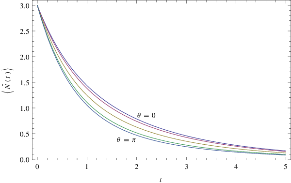
\Lambda_{t}\hat{N}=\frac{e^{-\Gamma_{1}t}+e^{-\Gamma_{2}t}}{2}\hat{N}+\frac{e^{-\Gamma_{1}t}-e^{-\Gamma_{2}t}}{2}[\hat{S}\cos\theta+\hat{Q}_{+}\sin\theta]\,,

(50)

where $\hat{Q}_{+}=\hat{a}_{1}^{\dagger}\hat{a}_{2}e^{i\phi}+\hat{a}_{2}^{\dagger}\hat{a}_{1}e^{-i\phi}$ , so the mean value in the state $\ket{n_{1},n_{2}}$ is the following

\left<N(t)\right>=\frac{e^{-\Gamma_{1}t}+e^{-\Gamma_{2}t}}{2}(n_{1}+n_{2})+\frac{e^{-\Gamma_{1}t}-e^{-\Gamma_{2}t}}{2}(n_{1}-n_{2})\cos\theta

(51)

and is depicted in the Fig. 1.

Refer to caption — Figure 1: Number of particles for system with two flavours for mixing angles $\theta=0,\frac{\pi}{4},\frac{\pi}{2},\frac{3\pi}{4},\pi$ (from right to left) with $n_{1}=2$ and $n_{2}=1$ , and $\Gamma_{1}<\Gamma_{2}$ (time unit is $\tau=1/\Gamma$ ).

Similarly, for the strangeness (or lepton number) we get

\Lambda_{t}\hat{S}=\frac{e^{-\Gamma_{1}t}-e^{-\Gamma_{2}t}}{2}\hat{N}\cos\theta+e^{-\Gamma t}\sin(\Delta mt)\hat{Q}_{-}\sin\theta\\ +\left[\frac{e^{-\Gamma_{1}t}+e^{-\Gamma_{2}t}}{2}\cos^{2}\theta+e^{-\Gamma t}\cos(\Delta mt)\sin^{2}\theta\right]\hat{S}\\ +\left[\frac{e^{-\Gamma_{1}t}+e^{-\Gamma_{2}t}}{2}-e^{-\Gamma t}\cos(\Delta mt)\right]\hat{Q}_{+}\sin\theta\cos\theta\,,

(52)

where $\hat{Q}_{-}=i(\hat{a}_{1}^{\dagger}\hat{a}_{2}e^{i\phi}-\hat{a}_{2}^{\dagger}\hat{a}_{1}e^{-i\phi})$ , $\Gamma=\frac{1}{2}(\Gamma_{1}+\Gamma_{2})$ and $\Delta m=m_{2}-m_{1}$ . The mean value of this observable in the state $\ket{n_{1},n_{2}}$ is

\left<S(t)\right>=\frac{e^{-\Gamma_{1}t}-e^{-\Gamma_{2}t}}{2}(n_{1}+n_{2})\cos\theta\\ +\left[\frac{e^{-\Gamma_{1}t}+e^{-\Gamma_{2}t}}{2}\cos^{2}\theta+e^{-\Gamma t}\cos(\Delta mt)\sin^{2}\theta\right](n_{1}-n_{2})

(53)

and is shown in the Fig. 2.

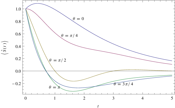
Let us pay our attention on the two extreme cases: $\theta=0$ (no flavour mixing) and $\theta=\frac{\pi}{2}$ (maximal mixing). For $\theta=0$ we have $\hat{c}_{i}=\hat{a}_{i}$ , so the time evolution of the observables is


$\displaystyle\Lambda_{t}\hat{N}$	$\displaystyle=\frac{1}{2}e^{-\Gamma_{1}t}(\hat{N}+\hat{S})+\frac{1}{2}e^{-\Gamma_{2}t}(\hat{N}-\hat{S})\,,$	(54a)
$\displaystyle\Lambda_{t}\hat{S}$	$\displaystyle=\frac{1}{2}e^{-\Gamma_{1}t}(\hat{S}+\hat{N})+\frac{1}{2}e^{-\Gamma_{2}t}(\hat{S}-\hat{N})\,.$	(54b)

Their mean values in the state $\ket{n_{1},n_{2}}$ are


$\displaystyle\left<N(t)\right>$	$\displaystyle=e^{-\Gamma_{1}t}n_{1}+e^{-\Gamma_{2}t}n_{2}\,,$	(55a)
$\displaystyle\left<S(t)\right>$	$\displaystyle=e^{-\Gamma_{1}t}n_{1}-e^{-\Gamma_{2}t}n_{2}\,.$	(55b)

For $\theta=\frac{\pi}{2}$ , $\phi=2\pi$ , $\psi=\pi$ and $\chi=\frac{3\pi}{2}$ we have

	$\displaystyle\hat{c}_{1}^{\dagger}$	$\displaystyle=\frac{1}{\sqrt{2}}(\hat{a}_{1}^{\dagger}+\hat{a}_{2}^{\dagger})\,,$
	$\displaystyle\hat{c}_{2}^{\dagger}$	$\displaystyle=\frac{1}{\sqrt{2}}(\hat{a}_{1}^{\dagger}-\hat{a}_{2}^{\dagger})\,,$

and the time evolution of the observables is given by


$\displaystyle\Lambda_{t}\hat{N}$	$\displaystyle=\frac{1}{2}\left(e^{-\Gamma_{1}t}+e^{-\Gamma_{2}t}\right)\hat{N}+\frac{1}{2}\left(e^{-\Gamma_{1}t}-e^{-\Gamma_{2}t}\right)\hat{Q}_{+}\,,$	(56a)
$\displaystyle\Lambda_{t}\hat{S}$	$\displaystyle=e^{-\Gamma t}\cos(\Delta mt)\hat{S}+e^{-\Gamma t}\sin(\Delta mt)\hat{Q}_{-}\,.$	(56b)

The mean values of these observables in the state $\ket{n_{1},n_{2}}$ are


$\displaystyle\left<N(t)\right>$	$\displaystyle=\frac{1}{2}\left(e^{-\Gamma_{1}t}+e^{-\Gamma_{2}t}\right)(n_{1}+n_{2})\,,$	(57a)
$\displaystyle\left<S(t)\right>$	$\displaystyle=e^{-\Gamma t}\cos(\Delta mt)(n_{1}-n_{2})\,,$	(57b)

so we get oscillations of the quantum number $S$ . It is worth noting, that for the particles such as $K$ or $B$ mesons we can use this result only as a first approximation, since for these particles the transformation which “diagonalizes” the master equation is non-unitary due to $CP$ -violation. For the sake of brevity, we do not discuss the violated $CP$ -symmetry here but preliminary calculations show the agreement with values for masses and life-times of neutral $K$ or $B$ mesons estimated on the basis of traditional Wigner–Weisskopf approach.

V Conclusions

We have analyzed a class of master equations built up from creation and annihilation operators which generate dynamical semigroups that can describe the exponential decay and flavour oscillations for system of many particles. We have shown, in this case, how this dynamical semigroup can be written in the Schrödinger as well as Heisenberg picture. This allowed us to choose the picture which seems to be more convenient for the description of the system under consideration. Moreover, we have found the solution for a free particle master equation in the form of Kraus representation in the language of annihilation and creation operators. Although, this Kraus representation is given by an infinite series, in the Schrödinger picture it reduces to a finite sum, whenever the initial state has a finite number of particles. On the other hand, in the Heisenberg picture the commutation relations between observables and Kraus operators sometimes allows us to find the observable evolution in closed form without explicit summation of the series.

Notice that if we cut the presented approach to the one-zero particle sector we get the theory given in [35] (neglecting the decoherence).

In the present paper we restrict our analysis only to states labeled by a discrete index, and not by continuous parameter (like e.g. momentum). Despite the fact that introducing a continuous parameter causes creation and annihilation operators to become operator-valued distributions, it seems to us that the approach introduced here should also be applicable.

We left open the question whether it is possible to apply our approach to describe the processes other than exponential decay, like e.g. decoherence or different decay laws. The preliminary investigations suggest that there exists a positive answer.

Acknowledgments

This work was supported by the Polish Ministry of Science and Higher Education under Contract No. NN202 103738.

References

[1] V. Weisskopf and E. Wigner, Z. Phys. 63, 54 (1930a).
[2] V. Weisskopf and E. Wigner, Z. Phys. 65, 18 (1930b).
[3] T. Durt, Int. J. Mod. Phys. B 27, 1345015 (2013).
[4] F. Uchiyama, Phys. Lett. A 231, 295 (1997).
[5] A. Bramon and M. Nowakowski, Phys. Rev. Lett. 83, 1 (1999).
[6] R. Foadi and F. Selleri, Phys. Rev. A 61, 012106 (1999).
[7] R. H. Dalitz and G. Garbarino, Nucl. Phys. B 606, 483 (2001).
[8] R. Bertlmann, W. Grimus, and B. C. Hiesmayr, Phys. Lett. A 289, 21 (2001).
[9] R. A. Bertlmann and B. C. Hiesmayr, Phys. Rev. A 63, 062112 (2001).
[10] A. Bramon and G. Garbarino, Phys. Rev. Lett. 89, 160401 (2002).
[11] R. A. Bertlmann, K. Durstberger, and B. C. Hiesmayr, Phys. Rev. A 68, 012111 (2003).
[12] M. Genovese, Phys. Rev. A 69, 022103 (2004).
[13] A. Go, J. Mod. Opt. 51, 991 (2004).
[14] A. Bramon, R. Escribano, and G. Garbarino, J. Mod. Opt. 52, 1681 (2005).
[15] A. Go et al., Phys. Rev. Lett. 99, 131802 (2007).
[16] F. Benatti and R. Floreanini, Phys. Lett. B 389, 100 (1996).
[17] F. Benatti and R. Floreanini, Nucl. Phys. B 488, 335 (1997a).
[18] F. Benatti and R. Floreanini, Phys. Lett. B 401, 337 (1997b).
[19] F. Benatti and R. Floreanini, Nucl. Phys. B 511, 550 (1998a).
[20] F. Benatti and R. Floreanini, Phys. Rev. D 57, R1332 (1998b).
[21] F. Benatti, in Irreversibility and Causality Semigroups and Rigged Hilbert Spaces, Lecture Notes in Physics, Vol. 504, edited by A. Bohm, H.-D. Doebner, and P. Kielanowski (Springer, Berlin–Heidelberg, 1998) pp. 124–147.
[22] F. Benatti, R. Floreanini, and R. Romano, Nucl. Phys. B 602, 541 (2001).
[23] J. Ellis, J. L. Lopez, N. E. Mavromatos, and D. V. Nanopoulos, Phys. Rev. D 53, 3846 (1996).
[24] J. Bernabéu, N. E. Mavromatos, and P. Villanueva-Pérez, Phys. Lett. B 724, 269 (2013).
[25] A. Kossakowski, Rep. Math. Phys. 3, 247 (1972).
[26] V. Gorini, A. Kossakowski, and E. C. G. Sudarshan, J. Math. Phys. 17, 821 (1976).
[27] G. Lindblad, Commun. Math. Phys. 48, 119 (1976).
[28] A. Kossakowski, in Irreversibility and Causality Semigroups and Rigged Hilbert Spaces, Lecture Notes in Physics, Vol. 504, edited by A. Bohm, H.-D. Doebner, and P. Kielanowski (Springer, Berlin–Heidelberg, 1998) pp. 59–66.
[29] R. Alicki and M. Fannes, Quantum Dynamical Systems (Oxford University Press, 2001).
[30] H.-P. Breuer and F. Petruccione, The Theory of Open Quantum Systems (Oxford University Press, 2002).
[31] R. Alicki, Rep. Math. Phys. 11, 1 (1977).
[32] R. Alicki, Rep. Math. Phys. 14, 27 (1978).
[33] A. Weron, A. K. Rajagopal, and K. Weron, Phys. Rev. A 31, 1736 (1985).
[34] R. Alicki, in Quantum Dynamical Semigroups and Applications, Lecture Notes in Physics, Vol. 717, edited by R. Alicki and K. Lendi (Springer, Berlin–Heidelberg, 2007) pp. 1–46.
[35] P. Caban, J. Rembieliński, K. A. Smoliński, and Z. Walczak, Phys. Rev. A 72, 032106 (2005).
[36] R. A. Bertlmann, W. Grimus, and B. C. Hiesmayr, Phys. Rev. A 73, 054101 (2006).
[37] P. Caban et al., Phys. Lett. A 357, 6 (2006).
[38] P. Caban, J. Rembieliński, K. A. Smoliński, and Z. Walczak, Phys. Lett. A 363, 389 (2007).
[39] P. Caban, J. Rembieliński, K. A. Smoliński, and Z. Walczak, J. Phys. A: Math. Gen. 35, 3265 (2002).
[40] B. Demoen, P. Vanheuverzwijn, and A. Verbeure, Lett. Math. Phys. 2, 161 (1977).
[41] D. E. Evans and J. T. Lewis, J. Funct. Anal. 26, 369 (1977).
[42] P. Vanheuverzwijn, Ann. Inst. Henri Poincaré (A) 29, 123 (1978).
[43] D. E. Evans, Commun. Math. Phys. 70, 53 (1979).
[44] P. Blanchard, M. Hellmich, P. Ługiewicz, and R. Olkiewicz, J. Math. Phys. 48, 012106 (2007).
[45] P. Blanchard, M. Hellmich, P. Ługiewicz, and R. Olkiewicz, J. Funct. Anal. 256, 1453 (2009).
[46] P. Blanchard, M. Hellmich, P. Ługiewicz, and R. Olkiewicz, J. Funct. Anal. 259, 2455 (2010).
[47] M. Hellmich, Rep. Math. Phys. 66, 277 (2010).
[48] R. Olkiewicz and M. Żaba, Phys. Lett. A 327, 3176 (2008a).
[49] R. Olkiewicz and M. Żaba, Phys. Lett. A 327, 4985 (2008b).
[50] Y.-H. M. Q.-X. Mu, G.-H. Yang, and L. Zhou, J. Phys. B: At. Mol. Opt. Phys. 41, 215502 (2008).
[51] R. Olkiewicz and M. Żaba, J. Phys. B: At. Mol. Opt. Phys. 42, 205540 (2009).
[52] K. Kraus, States, Effects and Operations (Springer, Berlin, 1983).
[53] Y.-X. Liu, Ş. K. Özdemir, A. Miranowicz, and N. Imoto, Phys. Rev. A 70, 042308 (2004).
[54] I. L. Chuang, D. W. Leung, and Y. Yamamoto, Phys. Rev. A 56, 1114 (1997).