Approximate Closest Community Search in Networks

Xin Huang^†, Laks V.S. Lakshmanan^†, Jeffrey Xu Yu^‡, Hong Cheng^‡
^† University of British Columbia ^‡The Chinese University of Hong Kong
{xin0 laks}@cs.ubc.ca {yu hcheng}@se.cuhk.edu.hk

Abstract

Recently, there has been significant interest in the study of the community search problem in social and information networks: given one or more query nodes, find densely connected communities containing the query nodes. However, most existing studies do not address the “free rider” issue, that is, nodes far away from query nodes and irrelevant to them are included in the detected community. Some state-of-the-art models have attempted to address this issue, but not only are their formulated problems NP-hard, they do not admit any approximations without restrictive assumptions, which may not always hold in practice.

In this paper, given an undirected graph $G$ and a set of query nodes $Q$ , we study community search using the $k$ -truss based community model. We formulate our problem of finding a closest truss community (CTC), as finding a connected $k$ -truss subgraph with the largest $k$ that contains $Q$ , and has the minimum diameter among such subgraphs. We prove this problem is NP-hard. Furthermore, it is NP-hard to approximate the problem within a factor $(2-\varepsilon)$ , for any $\varepsilon>0$ . However, we develop a greedy algorithmic framework, which first finds a CTC containing $Q$ , and then iteratively removes the furthest nodes from $Q$ , from the graph. The method achieves 2-approximation to the optimal solution. To further improve the efficiency, we make use of a compact truss index and develop efficient algorithms for $k$ -truss identification and maintenance as nodes get eliminated. In addition, using bulk deletion optimization and local exploration strategies, we propose two more efficient algorithms. One of them trades some approximation quality for efficiency while the other is a very efficient heuristic. Extensive experiments on 6 real-world networks show the effectiveness and efficiency of our community model and search algorithms.

1 Introduction

Community structures naturally exist in many real-world networks such as social, biological, collaboration, and communication networks. The task of community detection is to identify all communities in a network, which is a fundamental and well-studied problem in the literature. Recently, several papers have studied a related but different problem called community search, which is to find the community containing a given set of query nodes. The need for community search naturally arises in many real application scenarios, where one is motivated by the discovery of the communities in which given query nodes participate. Since the communities defined by different nodes in a network may be quite different, community search with query nodes opens up the prospects of user-centered and personalized search, with the potential of the answers being more meaningful to a user [17]. As just one example, in a social network, the community formed by a person’s high school classmates can be significantly different from the community formed by her family members which in turn can be quite different from the one formed by her colleagues [21].

Refer to caption — Figure 1: Closest truss community example

Various community models have been proposed based on different dense subgraph structures such as $k$ -core [27, 10, 20] , $k$ -truss [17], quasi-clique [9], weighted densest subgraph [32], to name a few major examples. Of these, the $k$ -truss as a definition of cohesive subgraph of a graph $G$ , requires that each edge be contained in at least $(k-2)$ triangles within this subgraph. Consider the graph $G$ in Figure 1; in the subgraph in the whole grey region (i.e., excluding the node $t$ ), each edge is contained in two triangles. Thus, the subgraph is a 4-truss. It is well known that most of real-world social networks are triangle-based, which always have high local clustering coefficient. Triangles are known as the fundamental building blocks of networks [29]. In a social network, a triangle indicates two friends have a common friend, which shows a strong and stable relationship among three friends. Intuitively, the more common friends two people have, the stronger their relationship. In a $k$ -truss, each pair of friends is “endorsed” by at least $(k-2)$ common friends. Thus, a $k$ -truss with a large value of $k$ signifies strong inner-connections between members of the subgraph. Huang et al. [17] proposed a community model based on the notion of $k$ -truss as follows. Given one query node $q$ and a parameter $k$ , a $k$ -truss community containing $q$ is a maximal $k$ -truss containing $q$ , in which each edge is “triangle connected” with other edges. Triangle connectivity is strictly stronger than connectivity. The $k$ -truss community model works well to find all overlapping communities containing a query node $q$ . It is natural to search for communities containing a set of query nodes in real applications, and the above community model, extended for multiple query nodes, has the following limitations. Due to the strict requirement of triangle connectivity constraint, the model may fail to discover any community for query nodes. For example, for the graph of Figure 1(a), and query nodes $Q=\{v_{4},q_{3},p_{1}\}$ the above $k$ -truss community model cannot find a qualified community for any $k$ , since the edges $(v_{4},q_{3})$ and $(q_{3},p_{1})$ are not triangle connected in any $k$ -truss. A detailed comparison of various community search models and techniques can be found in the Section 7.

In this paper, we study the problem of close community search, i.e., given a set of query nodes, find a dense connected subgraph that contains the query nodes, in which nodes are close to each other. As a qualifying cohesive structure, we use the notion of $k$ -truss for modeling a densely connected community, which inherits several good structural properties, such as $k$ -edge connectivity, bounded diameter and hierarchical structure. In addition, to ensure every node included in the community is tightly related to query nodes and other nodes included in the community reported, we use graph diameter to measure the closeness of all nodes in the community. Thus, based on $k$ -truss and graph diameter, we propose a novel community model as closest truss community (CTC), which requires that the all query nodes are connected in this community, the graph structure is a $k$ -truss with the largest trussness $k$ . In general, several such candidate communities may exist. Some of them may suffer from the so-called “free rider effect” formally defined and studied in [32]. While we discuss this in detail in Section 3.2, we illustrate it with an example here. In Figure 1(a), for the query nodes $\{q_{1},q_{2},q_{3}\}$ , the subgraph shaded grey is a 4-truss containing the query nodes. It includes the nodes $p_{1},p_{2},p_{3}$ which are intuitively not relevant to the query nodes. Specifically, they are all far away from $q_{1}$ and can be regarded as “free riders”. This 4-truss is said to suffer from the free rider effect. On the other hand, the subgraph without the nodes $\{p_{1},p_{2},p_{3}\}$ is also a 4-truss, it has the smallest diameter among all 4-trusses containing the query nodes, and does not suffer from the free rider effect. Motivated by this, we define a closest truss community as a connected $k$ -truss with the largest $k$ containing the query nodes and having the smallest diameter. We show that such a definition avoids the free rider effect. A connected $k$ -truss with the largest $k$ containing given query nodes can be found in polynomial time. However, as we show, finding such a $k$ -truss with the minimum diameter is NP-hard and it is hard to approximate within a factor better than 2. Here, the approximation is w.r.t. the minimum diameter. On the other hand, we develop a greedy strategy for finding a CTC that delivers a 2-approximation to the optimal solution, thus essentially matching the lower bound. In order to make our algorithm scalable to large real networks, we propose two techniques. One of them is based on bulk deletion of nodes far away from query nodes. The second is a heuristic exploration of the local neighborhood of a Steiner tree containing the query nodes. The challenge here is that a naive application of Steiner trees may yield a $k$ -truss with a low value of $k$ , which is undesirable. We address this challenge by developing a new notion of distances based on edge trussness. Specifically, we make the following contributions in this paper.

•

We propose a novel community search model called closest truss community (CTC) and motivate the problem of finding CTC containing given query nodes (Section 2).
•

We analyze the structural and computational properties of CTC and show that it avoids the free rider effect, is NP-hard to compute exactly or to approximate within a factor of $(2-\varepsilon)$ , for any $\varepsilon>0$ (Section 3).
•

We develop a greedy 2-approximation algorithm for finding a CTC given a set of query nodes. The algorithm is based on finding, in linear time, a connected $k$ -truss with maximum $k$ containing the query nodes, using a simple truss index. Then successively nodes far away from the query nodes are eliminated (Section 4).
•

We further speed up CTC search in two ways: (1) we make use of a clever bulk deletion strategy and (2) find a Steiner tree of the query nodes and expand it into a $k$ -truss by exploring the local neighborhood of the Steiner tree. The first of these slightly degrades the approximation factor while the second is a heuristic (Section 5).
•

We extensively experiment with the various algorithms on 6 real networks. Our results show that our $\mathsf{closest}$ $\mathsf{truss}$ $\mathsf{community}$ model can efficiently and effectively discover the queried communities on real-world networks with ground-truth communities. (Section 6).

In Section 7, we present a detailed comparison with related work. In Section 7.1, we discuss alternative candidates for community models and provide a rationale for our design decisions. We summarize the paper in Section 8.

2 Problem Definition

We consider an undirected, unweighted simple graph $G=(V(G),$ $E(G))$ with $n=|V(G)|$ vertices and $m=|E(G)|$ edges. We denote the set of neighbors of a vertex $v$ by $N(v)$ , i.e., $N(v)=\{u\in V:(v,u)\in E\}$ , and the degree of $v$ by $d(v)=|N(v)|$ . We use $d_{max}=\max_{v\in V}d(v)$ to denote the maximum vertex degree in $G$ . W.l.o.g we assume in this paper that the graph $G$ we consider is connected. Note that this implies that $m\geq n-1$ . Table 1 summarizes the frequently used notations in the paper.

A triangle in $G$ is a cycle of length 3. Let $u,v,w\in V$ be the three vertices on the cycle, then we denote this triangle by $\triangle_{uvw}$ . The support of an edge $e(u,v)\in E$ in $G$ , denoted $sup_{G}(e)$ , is defined as $|\{\triangle_{uvw}:w\in V\}|$ . When the context is obvious, we drop the subscript and denote the support as $sup(e)$ . Based on the definition of $k$ -truss [7, 29], we define a connected $k$ -truss as follows.

Table 1: Frequently Used Notations

Notation	Description
$G=(V(G),E(G))$	An undirected and connected simple graph $G$
$n;m$	The number of vertices/edges in $G$
$N(v)$	The set of neighbors of $v$
$\sup_{H}(e)$	The support of edge $e$ in $H$
$\tau(H)$	Trussness of graph $H$
$\tau(e)$	Trussness of edge $e$
$\tau(v)$	Trussness of vertex $v$
$\bar{\tau}(S)$	The maximum trussness of connected graphs containing $S$
${\mathsf{diam}}(H)$	The diameter of graph $H$
${\mathsf{dist}}_{H}(v,u)$	The shortest distance between $v$ and $u$ in $H$
${\mathsf{dist}}_{H}(R,Q)$	${\mathsf{dist}}_{H}(R,Q)=\max_{v\in R,u\in Q}{\mathsf{dist}}_{H}(v,u)$

Definition 1 (Connected K-Truss)

Given a graph $G$ and an integer $k$ , a connected $k$ -truss is a connected subgraph $H\subseteq G$ , such that $\forall e\in E(H)$ , $sup_{H}(e)$ $\geq(k-2)$ .

Intuitively, a connected $k$ -truss is a connected subgraph such that each edge $(u,v)$ in the subgraph is “endorsed” by $k-2$ common neighbors of $u$ and $v$ [7]. In a connected $k$ -truss graph, each node has degree at least $k-1$ and a connected $k$ -truss is also a $(k-1)$ -core [2]. Next, we define the trussness of a subgraph, an edge, and a vertex as follows.

Definition 2 (Trussness)

The trussness of a subgraph $H$ $\subseteq$ $G$ is the minimum support of an edge in $H$ plus $2$ , i.e., $\tau(H)=2+\min_{e\in E(H)}\{sup_{H}(e)\}$ . The trussness of an edge $e\in E(G)$ is $\tau(e)=\max_{H\subseteq G\wedge e\in E(H)}\{\tau(H)\}$ . The trussness of a vertex $v\in V(G)$ is $\tau(v)=\max_{H\subseteq G\wedge v\in V(H)}$ $\{\tau(H)\}$ .

Consider the graph $G$ in Figure 1(a). Edge $e(q_{2},v_{2})$ is contained in three triangles $\triangle_{q_{2}v_{2}q_{1}}$ , $\triangle_{q_{2}v_{2}v_{1}}$ and $\triangle_{q_{2}v_{2}v_{5}}$ , thus its support is $sup_{G}(e(q_{2},v_{2}))=3$ . Suppose $H$ is the triangle $\triangle_{q_{2}v_{2}q_{1}}$ , then the trussness of the subgraph $H$ is $\tau(H)=2+\min_{e\in H}{sup_{H}(e)}=3$ , since each edge is contained in one triangle in $H$ . The trussness of the edge $e(q_{2},v_{2})$ is 4, because in the induced subgraph on vertices $\{q_{1},q_{2},v_{1},v_{2}\}$ , each edge is contained in two triangles in the subgraph and any subgraph $H$ containing $e(q_{2},v_{2})$ has $\tau(H)\leq 4$ , i.e., $\tau(e(q_{2},v_{2}))=$ $\max_{H\subseteq G\wedge e\in E(H)}$ $\{\tau(H)\}$ $=4$ . Note that the trussness of an edge $e$ of a graph $G$ could be less than $sup_{G}(e)+2$ , e.g., $\tau(e(q_{2},v_{2}))$ $=4<5$ $=sup(e(q_{2},v_{2}))+2$ . Moreover, the vertex trussness of $q_{2}$ is also 4, i.e. $\tau(q_{2})=4$ .

For a set of vertices $S\subseteq V(G)$ , we use $\bar{\tau}(S)$ to denote the maximum trussness of a conncted subgraph $H$ containing $S$ , i.e., $\bar{\tau}(S)=\max_{S\subseteq H\subseteq G\wedge H\text{is connected}}$ $\{\tau(H)\}$ . Notice that by definition, for $S=\emptyset$ , $\bar{\tau}(\emptyset)$ is the maximum trussness of any edge in $G$ . In Figure 1(a), the whole subgraph in the grey region is a 4-truss. There exists no 5-truss in $G$ , and $\bar{\tau}(\emptyset)=4$ . We will make use of $\bar{\tau}(\emptyset)$ in Section 5.

For two nodes $u,v\in G$ , we denote by ${\mathsf{dist}}_{G}(u,v)$ the length of the shortest path between $u$ and $v$ in $G$ , where ${\mathsf{dist}}_{G}(u,v)=+\infty$ if $u$ and $v$ are not connected. We make use of the notions of graph query distance and diamater in the rest of the paper.

Definition 3 (Query Distance)

Given a graph $G$ and a set of query nodes $Q\subset V$ , for each vertex $v\in G$ , the vertex query distance of $v$ is the maximum length of a shortest path from $v$ to a query node $q\in Q$ , i.e., ${\mathsf{dist}}_{G}(v,Q)=\max_{q\in Q}$ ${\mathsf{dist}}_{G}(v,q)$ . For a subgraph $H\subseteq G$ , the graph query distance of $H$ is defined as ${\mathsf{dist}}_{G}(H,Q)=$ $\max_{u\in H}{\mathsf{dist}}_{G}(u,Q)$ $=\max_{u\in H,q\in Q}{\mathsf{dist}}_{G}(u,q).$

Definition 4 (Graph Diameter)

The diameter of a graph $G$ is defined as the maximum length of a shortest path in $G$ , i.e., ${\mathsf{diam}}(G)=\max_{u,v\in G}\{{\mathsf{dist}}_{G}(u,v)\}$ .

For the graph $G$ in Figure 1(a) and $Q=\{q_{2},$ $q_{3}\}$ , the vertex query distance of $v_{2}$ is ${\mathsf{dist}}_{G}(v_{2},Q)=$ $\max_{q\in Q}$ $\{dist_{G}(v_{2},q)\}$ $=2$ , since ${\mathsf{dist}}_{G}(v_{2},q_{3})=2$ and ${\mathsf{dist}}_{G}(v_{2},q_{2})=1$ . Let $H$ be the subgraph of Figure 1(a) shaded in grey. Then query distance of $H$ is ${\mathsf{dist}}_{G}(H,Q)=3$ . The diameter of $H$ is ${\mathsf{diam}}(H)=4$ .

On the basis of the definitions of $k$ -truss and graph diameter, we define the closest truss community in a graph $G$ as follows.

Definition 5 (Closest Truss Community)

Given a graph $G$ and a set of query nodes $Q$ , $G^{\prime}$ is a closest truss community (CTC), if $G^{\prime}$ satisfies the following two conditions:

(1) Connected $k$ -Truss.: $G^{\prime}$ is a connected $k$ -truss containing $Q$ with the largest $k$ , i.e., $Q\subseteq$ $G^{\prime}$ $\subseteq G$ and $\forall e\in E(G^{\prime})$ , $sup(e)\geq k-2$ ;
(2) Smallest Diameter.: $G^{\prime}$ is a subgraph of smallest diameter satisfying condition (1). That is, $\nexists G^{\prime\prime}\subseteq G$ , such that $diam(G^{\prime\prime})$ $<diam(G^{\prime})$ , and $G^{\prime\prime}$ satisfies condition (1).

Condition (1) requires that the closest community containing the query nodes $Q$ be densely connected. In addition, Condition (2) makes sure that each node is as close as possible to every other node in the community, including the query nodes. We next illustrate the notion of CTC as well as the consequence of considering Conditions (1) and (2) in different order.

Example 1

In Definition 5, we firstly consider the connected $k$ -truss of $G$ containing query nodes with the largest trussness, and then among such subgraphs, regard the one with the smallest diameter as the $\mathsf{closest}$ $\mathsf{truss}$ $\mathsf{community}$ . Consider the graph $G$ in Figure 1(a), and $Q=\{q_{1},q_{2},q_{3}\}$ ; the subgraph in the region shaded grey is a 4-truss containing $Q$ , and is a subgraph with the largest trussness that contains $Q$ , and has diameter 4. Notice that in Figure 1(a), although the nodes $p_{1},p_{2},p_{3}$ belong to the 4-truss and are strongly connected with $q_{3}$ , they are far away from the query node $q_{1}$ . Figure 1(b) shows another 4-truss containing $Q$ but not $p_{1},p_{2},p_{3}$ , and its diameter is 3. It can be verified that this is the 4-truss with the smallest diameter. Thus, by Condition (2) of Definition 5, the 4-truss graph in Figure 1(a) will not be regarded the closest truss community, whereas the one in Figure 1(b) is indeed the CTC. Intuitively, the nodes $p_{1},p_{2},p_{3}$ are “free riders” that belong to a community defined only using Condition (1), and are avoided by Condition (2). We will see in Section 3.2 that the definition of CTC above avoids the so-called “free rider effect”. \qed

Example 2

Suppose we apply the conditions in Definition 5 in the opposite order. That is, we first minimize the diameter among connected subgraphs of $G$ containing $Q$ and look for the $k$ -truss subgraph with the largest $k$ among those. Firstly, we find that the cycle of $\{(q_{1},t),$ $(t,q_{3}),$ $(q_{3},v_{4}),$ $(v_{4},q_{2}),$ $(q_{2},q_{1})\}$ is the connected subgraph containing $Q$ with the smallest diameter 2. Then, we find that this cycle is also the $k$ -truss subgraph with the largest $k$ containing itself. However, it is only a 2-truss, which has a loosely connected structure compared to Figure 1(b). This justifies the choice of the order in which Conditions (1) and (2) should be applied. \qed

We discuss several natural candidates for community models in Section 7.1 and provide a rationale for our design decisions. We have a choice between minimizing diameter or minimizing query distance. We address this choice in Section 3.2: Example 3.5 illustrates the value added by minimizing the diameter over minimizing just the query distance. The problem of closest truss community (CTC) search studied in this paper is stated as follows.

Problem 1 ( $\mathsf{CTC}$ - $\mathsf{Problem}$ )

Given a graph $G(V,E)$ and a set of query vertices $Q=\{v_{1},...,v_{r}\}\subseteq V$ , find a closest truss community containing $Q$ .

3 Problem Analysis

3.1 Structural Properties

Since our closest truss community model is based on the concept of $k$ -truss, the communities caputure good structral properties of $k$ -truss, such as k-edge-connected and hierarchical structure. In addition, since CTC is required to have minimum diameter, it also has bounded diameter. As a result, CTC avoids the “free rider effect” [27, 32] (see Section 3.2).

Small diameter, k-edge-connected, hierarchical structure. First, the diameter of a connected $k$ -truss with $n$ vertices is no more than $\lfloor\frac{2n-2}{k}\rfloor$ [7]. The diameter of a community is considered as an important feature of a community [12]. Moreover, a $k$ -truss community is ( $k-1$ )-edge-connected [7], as it remains connected whenever fewer than $k-1$ edges are removed [14]. In addition, $k$ -truss based community has hierarchical structure that represents the cores of a community at different levels of granularity [17], that is, $k$ -truss is always contained in the $(k-1)$ -truss for any $k\geq 3$ .

Largest $k$ . We have a trivial upper bound on the maximum possible trussness of a connected $k$ -truss containing the query nodes.

Lemma 1

For a connected $k$ -truss $H$ satisfying definition of CTC for $Q$ , we have $k\leq\min$ $\{\tau(q_{1}),$ $...,\tau(q_{r})\}$ holds.

Proof 3.1.

First, we have $Q\subseteq H$ . For each node $q\in Q$ , $q$ cannot be contained in a $k$ -truss in $G$ , whenever $k>\tau(q)$ . Thus, the fact that $H$ is a $k$ -truss subgraph containing $Q$ implies that $k\leq$ $\min\{\tau(q_{1}),$ $...,\tau(q_{r})\}$ .

Lower and upper bounds on diameter. Since the distance function satisfies the triangular inequality, i.e., for all nodes $u,v,w$ , ${\mathsf{dist}}_{G}(u,v)\leq{\mathsf{dist}}_{G}(u,w)+{\mathsf{dist}}_{G}(w,v)$ , we can express the lower and upper bounds on the graph diameter in terms of the query distance as follows.

Lemma 3.2.

For a graph $G(V,E)$ and a set of nodes $Q\subseteq G$ , we have ${\mathsf{dist}}_{G}(G,Q)\leq{\mathsf{diam}}(G)\leq 2{\mathsf{dist}}_{G}(G,Q)$ .

Proof 3.3.

First, the diameter ${\mathsf{diam}}(G)=\max_{v,u\in G}{\mathsf{dist}}_{G}(v,u)$ , which is clearly no less than than ${\mathsf{dist}}_{G}(G,Q)=\max_{v\in G,q\in Q}$ ${\mathsf{dist}}_{G}(v,q)$ for $Q\subseteq G$ . Thus, ${\mathsf{dist}}_{G}(G,Q)\leq{\mathsf{diam}}(G)$ . Second, suppose that the longest shortest path in $G$ is between $v$ and $u$ . Then $\forall q\in Q$ , then we have ${\mathsf{diam}}(G)={\mathsf{dist}}(v,u)\leq{\mathsf{dist}}(v,q)+$ ${\mathsf{dist}}(q,u)\leq$ $2{\mathsf{dist}}_{G}(G,Q)$ . The lemma follows.

3.2 Free Rider Effect

In previous work on community detection, researchers [27, 32] have identified an undesirable phenomenon called “free rider effect”. Intuitively, if a definition of community admits irrelevant subgraphs in the detected community, we refer to such irrelevant subgraphs as free riders. For instance, suppose we use the classic density definition of average internal degree $\frac{|E|}{|V|}$ as the community goodness metric. Then for a set of query nodes $Q$ , the community is a subgraph containing $Q$ with the maximum density. Then, any local community for $Q$ merged with the densest subgraph part will increase the community density. However, the densest subgraph may be disconnected from or irrelvant to query nodes. This shows the simple density metric suffers from the free rider effect. Wu et al. [32] show that serveral other goodness metrics including minimum degree, local modularity, and external conductance suffer from the free rider effect. Following Wu et al. [32], we define the free rider effect as follows. Typically, a community definition is based on a goodness metric $f(H)$ for a subgraph $H$ : subgraphs with minimum¹¹ 1 We use minimum w.l.o.g. $f(H)$ value are defined as communities. E.g., for our CTC problem, diameter is the goodness metric: among all subgraphs with maximum trussness, the smaller the diameter of $H$ , the better it is as a community. The definition of free rider effect is based on this goodness metric. We term a community query independent if it is the solution to the community search with $Q$ set to $\emptyset$ .

Definition 3.4 ( $\mathsf{FRE}$ ).

Given a non-empty query $Q$ , let $H$ be a solution to a community definition based on a goodness metric $f(.)$ . Let $H^{*}$ be a (global or local) optimum solution, which is query-independent. If $f(H\cup H^{*})\leq f(H)$ , we say that the definition suffers from free rider effect. Here, nodes in $H^{*}\setminus H$ are called free riders for the query $Q$ and community $H$ .

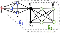
Example 3.5.

Consider Figure 2, showing a graph $G$ and query nodes $Q=\{q_{1},q_{2}\}$ . It also shows subgraphs $G_{1}$ and $G_{2}$ . All three graphs – $G,G_{1}$ , and $G_{2}$ – are 4-trusses containing $Q$ . The query distance of the star node $r$ is 3, while that for all other nodes is at most 2. Thus, the query distance of $G$ is 3. The subgraph $G_{1}$ has the minimum query distance 2 among all 4-trusses containing $Q$ . However, its diameter is 3, as the distance between square node $v$ and circle node $p$ is 3. On the other hand, the subgraph $G_{2}$ , while having the same query distance as $G_{1}$ , has a strictly smaller diameter 2. It has the minimum diameter among all 4-trusses containing $Q$ .

Both the star node and the square nodes are free riders. The star node is the furthest from query node $q_{2}$ and its removal from $G$ leaves the trussness unchanged. The square nodes have the same query distance 2 as the circle node $p$ . However, the square nodes are not close enough to other nodes of the community: e.g., their distance to circle node $p$ is 3. Unlike the circle nodes, removal of square nodes leaves the trussness unchanged. Thus, the square nodes are also free riders, while the circle nodes aren’t. Minimizing query distance among 4-trusses eliminates the free rider star node but not the square free rider nodes, while minimizing diameter eliminates both free riders. ∎

We next show that our definition of CTC avoids the problem of free rider effect.

In general, there may be multiple CTCs $H$ , i.e., connected $k$ -trusses with maximum trussness containing $Q$ with the minimum diameter. For example, consider the graph $G$ in Figure 1 and $Q=\{q_{3}\}$ . The subgraphs of $G$ induced respectively by $\{q_{3},p_{1},p_{2},p_{3}\}$ and $\{q_{3},v_{3},v_{4},v_{5}\}$ are both 4-trusses with diameter 1. Both happen to be maximal in that they are not contained in any other 4-truss with this property.

Proposition 3.6.

For any graph $G$ and query nodes $Q\subset V(G)$ , there is a solution $H$ to the CTC search problem such that for all query-independent optimal solutions $H^{*}$ , either $H^{*}=H$ , or $H\cup H^{*}$ is disconnected, or $H\cup H^{*}$ has a strictly larger diameter than $H$ .

Proof 3.7.

Let ${\cal C}(G,Q)$ denote the set of optimal solutions to the CTC search problem on graph $G$ and query nodes $Q$ . ${\cal C}(G,Q)$ is partially ordered w.r.t. the graph containment order $\subseteq$ . Let $H$ be any maximal element of ${\cal C}(G,Q)$ , let $H^{*}$ be any query-independent optimal solution, and consider $H\cup H^{*}$ . Assume w.l.o.g. that $(H^{*}\setminus H)\neq\emptyset$ . Suppose that $H\cup H^{*}$ is a connected $k$ -truss with maximum trussness containing $Q$ , and ${\mathsf{diam}}(H\cup H^{*})\leq{\mathsf{diam}}(H)$ . This contradicts the maximality of $H$ .

3.3 Hardness and Approximation

Hardness. In the following, we show the $\mathsf{CTC}$ - $\mathsf{Problem}$ is NP-hard. Thereto, we define the decision version of the $\mathsf{CTC}$ - $\mathsf{Problem}$ .

Problem 3.8 ( $\mathsf{CTCk}$ - $\mathsf{Problem}$ ).

Given a graph $G(V,E)$ , a set of query nodes $Q=\{v_{1},...,v_{r}\}\subseteq V$ and parameters $k$ and $d$ , test whether $G$ contains a connected $k$ -truss subgraph with diameter at most $d$ , that contains $Q$ .

Theorem 3.9.

The $\mathsf{CTCk}$ - $\mathsf{Problem}$ is NP-hard.

Proof 3.10.

We reduce the well-known NP-hard problem of Maximum Clique (decision version) to $\mathsf{CTCk}$ - $\mathsf{Problem}$ . Given a graph $G(V,E)$ and number $k$ , the Maximum Clique Decision problem is to check whether $G$ contains a clique of size $k$ . From this, construct an instance of $\mathsf{CTCk}$ - $\mathsf{Problem}$ , consisting of graph $G$ , parameters $k$ and $d=1$ , and the empty set of query nodes $Q=\emptyset$ . We show that the instance of the Maximum Clique Decision problem is a YES-instance iff the corresponding instance of $\mathsf{CTCk}$ - $\mathsf{Problem}$ is a YES-instance. Clearly, any clique with at least $k$ nodes is a connected $k$ -truss with diameter $1$ . On the other hand, given a solution $H$ for $\mathsf{CTCk}$ - $\mathsf{Problem}$ , $H$ must contain at least $k$ nodes since $H$ is a $k$ -truss, and $diam(H)=d=1$ , which implies $H$ is a clique.

The hardness of $\mathsf{CTC}$ - $\mathsf{Problem}$ follows from this. The next natural question is whether $\mathsf{CTC}$ - $\mathsf{Problem}$ can be approximated.

Approximation. For $\alpha\geq 1$ , we say that an algorithm achieves an $\alpha$ -approximation to the closest truss community (CTC) search problem if it outputs a connected $k$ -truss subgraph $H\subseteq G$ such that $Q\subseteq H$ , $\tau(H)=\tau(H^{*})$ and ${\mathsf{diam}}(H)\leq\alpha\cdot{\mathsf{diam}}(H^{*})$ , where $H^{*}$ is the optimal CTC. That is, $H^{*}$ is a connected $k$ -truss with the largest $k$ s.t. $Q\subseteq H^{*}$ , and $diam(H^{*})$ is the minimum among all such CTCs containing $Q$ . Notice that the trussness of the output subgraph $H$ matches that of the optimal solution $H^{*}$ and that the approximation is only w.r.t. the diameter: the diameter of $H$ is required to be no more than $\alpha\cdot diam(H^{*})$ .

Non-Approximability. We next prove that $\mathsf{CTC}$ - $\mathsf{Problem}$ cannot be approximated within a factor better than $2$ . We establish this result through a reduction, again from the Maximum Clique Decision problem to the problem of approximating $\mathsf{CTC}$ - $\mathsf{Problem}$ , given $k$ . In the next section, we develop a $2$ -approximation algorithm for $\mathsf{CTC}$ - $\mathsf{Problem}$ , thus essentially matching this lower bound. Notice that the $\mathsf{CTC}$ - $\mathsf{Problem}$ with given parameter $k$ is essentially the $\mathsf{CTCk}$ - $\mathsf{Problem}$ .

Theorem 3.11.

Unless $\mathsf{P}$ = $\mathsf{NP}$ , for any $\varepsilon>0$ , the $\mathsf{CTC}$ - $\mathsf{Problem}$ with given parameter $k$ cannot be approximated in polynomial time within a factor $(2-\varepsilon)$ of the optimal.

Proof 3.12.

Suppose there exists a polynomial time algorithm $\mathbb{A}$ for the $\mathsf{CTC}$ - $\mathsf{Problem}$ with a given $k$ that provides a solution $H$ with an approximation factor $(2-\varepsilon)$ of the optimal solution $H^{*}$ . Set the query nodes $Q=\emptyset$ . By our assumption, we have $Q\subseteq H$ , $\tau(H)=\tau(H^{*})=k$ and ${\mathsf{diam}}(H)\leq(2-\varepsilon)\cdot{\mathsf{diam}}(H^{*})$ . Next, we use this approximation solution to exactly solve the Maximum Clique Decision problem as follows. Since the latter cannot be done in polynomial time unless $\mathsf{P}$ = $\mathsf{NP}$ , the theorem follows.

Run algorithm $\mathbb{A}$ on a given instance $G$ of the Maximum Clique Decision problem, with parameter $k$ and query nodes $Q=\emptyset$ . We claim that $G$ contains a clique of size $k$ iff $\mathbb{A}$ outputs a solution $H$ with $\tau(H)=k$ and $diam(H)=1$ . To see this, suppose $diam(H)=1$ , then the optimal solution $H^{*}$ has ${\mathsf{diam}}(H^{*})\leq{\mathsf{diam}}(H)=1$ , and $H^{*}$ is a connected $k$ -truss, which shows $H^{*}$ is a clique of size $k$ in $G$ . On the other hand, suppose $diam(H)\geq 2$ . Then we have $2\cdot{\mathsf{diam}}(H^{*})>(2-\varepsilon)\cdot{\mathsf{diam}}(H^{*})\geq{\mathsf{diam}}(H)\geq 2$ . Since diameter is an integer, we deduce that $diam(H^{*})\geq 2$ . In this case, $G$ cannot possibly contain a clique of size $k$ , for if it did, that clique would be the optimal solution to the $\mathsf{CTC}$ - $\mathsf{Problem}$ on $G$ , with parameter $k$ , whose diameter is $1$ , which contradicts the optimality of $H^{*}$ . Thus, using algorithm $\mathbb{A}$ , we can distinguish between the YES and NO instances of the Maximum Clique Decision problem. This was to be shown.

4 Algorithms

In this section, we present a greedy algorithm called $\mathsf{Basic}$ for the CTC search problem. Then, we show that this algorithm achieves a 2-approximation to the optimal result. Finally, we discuss procedures for an efficient implementation of the algorithm and analyze its time and space complexity.

4.1 Basic Algorithmic Framework

Here is an overview of our algorithm $\mathsf{Basic}$ . First, given a graph $G$ and query nodes $Q$ , we find a maximal connected $k$ -truss, denoted as $G_{0}$ , containing $Q$ and having the largest trussness. As $G_{0}$ may have a large diameter, we iteratively remove nodes far away from the query nodes, while maintaining the trussness of the remainder graph at $k$ .

Algorithm. Algorithm 1 outlines a framework for finding a closest truss community based on a greedy strategy. For query nodes $Q$ , we first find a maximal connected $k$ -truss $G_{0}$ that contains $Q$ , s.t. $k=\tau(G_{0})$ is the largest (line 1). Then, we set $l=0$ . For all $u\in G_{l}$ and $q\in Q$ , we compute the shortest distance between $u$ and $q$ (line 4), and obtain the vertex query distance ${\mathsf{dist}}_{G_{l}}(u,Q)$ . Among all vertices, we pick up a vertex $u^{*}$ with the maximum ${\mathsf{dist}}_{G_{l}}(u^{*},Q)$ , which is also the graph query distance ${\mathsf{dist}}_{G_{l}}(G_{l},Q)$ (lines 5-6). Next, we remove the vertex $u^{*}$ and its incident edges from $G_{l}$ , and delete any nodes and edges needed to restore the $k$ -truss property of $G_{l}$ (lines 7-8). We assign the updated graph as a new $G_{l}$ . Then, we repeat the above steps until $G_{l}$ does not have a connected subgraph containing $Q$ (lines 3-9). Finally, we terminate by outputting graph $R$ as the closest truss community, where $R$ is any graph $G^{\prime}\in\{G_{0},...,G_{l-1}\}$ with the smallest graph query distance ${\mathsf{dist}}_{G^{\prime}}(G^{\prime},Q)$ (line 10). Note that each intermediate graph $G^{\prime}\in\{G_{0},...,G_{l-1}\}$ is a $k$ -truss with the maximum trussness as required.

Example 4.13.

We apply Algorithm 1 on $G$ in Figure 1 for $Q=\{q_{1},$ $q_{2},$ $q_{3}\}$ . First, we obtain the 4-truss subgraph $G_{0}$ shaded in grey, using a procedure we will shortly explain. Then, we compute all shortest distances, and get the maximum vertex query distance as ${\mathsf{dist}}_{G_{0}}(p_{1},Q)=4$ , and $u^{*}=p_{1}$ . We delete node $p_{1}$ and its incident edges from $G_{0}$ ; we also delete $p_{2}$ and $p_{3}$ , in order to restore the 4-truss property. The resulting subgraph is $G_{1}$ . Any further deletion of a node in the next iteration of the while loop will induce a series of deletions in line 8, eventually making the graph disconnected or containing just a part of query nodes. As a result, the output graph $R$ , shown in Figure 1(b), is just $G_{1}$ . Also ${\mathsf{dist}}_{R}(R,Q)=3$ , and $R$ happens to be the exact CTC with diameter $3$ , which is optimal.

Algorithm 1

\mathsf{Basic}

(

G

Q

)

Input: A graph $G=(V,E)$ , a set of query nodes $Q=\{q_{1},...,q_{r}\}$ .
Output: A connected $k$ -truss $R$ with a small diameter.

1: Find a maximal connected

k

-truss containing

Q

with the largest

k

G_{0}

//see Algorithm 2.

l\leftarrow 0

;

3: while

{\mathsf{connect}}_{G_{l}}(Q)=

true do

4: Compute

{\mathsf{dist}}_{G_{l}}(q,u)

\forall q\in Q

and

\forall u\in G_{l}

;

u^{*}\leftarrow\arg\max_{u\in G_{l}}{\mathsf{dist}}_{G_{l}}(u,Q)

;

{\mathsf{dist}}_{G_{l}}(G_{l},Q)\leftarrow{\mathsf{dist}}_{G_{l}}(u^{*},Q)

;

7: Delete

u^{*}

and its incident edges from

G_{l}

;

8: Maintain

k

-truss property of

G_{l}

//see Algorithm 3;

G_{l+1}\leftarrow G_{l}

;

l\leftarrow l+1

;

10:

R\leftarrow\arg\min_{G^{\prime}\in\{G_{0},...,G_{l-1}\}}{{\mathsf{dist}}_{G^{\prime}}(G^{\prime},Q)}

;

4.2 Approximation Analysis

Algorithm 1 can achieve 2-approxiamtion to the optimal solution, that is, the obtained connected $k$ -truss community $R$ satisfies $Q\subseteq R$ , $\tau(R)=\tau(H^{*})$ and ${\mathsf{diam}}(R)\leq 2{\mathsf{diam}}(H^{*})$ , for any optimal solution $H^{*}$ . Since any graph in $\{G_{0},...,G_{l-1}\}$ is a connceted $k$ -truss with the largest $k$ containing $Q$ by Algorithm 1, and $R\in\{G_{0},...,G_{l-1}\}$ , we have $Q\subseteq R$ , and $\tau(R)=\tau(H^{*})$ . In the following, we will prove that ${\mathsf{diam}}(R)\leq 2{\mathsf{diam}}(H^{*})$ . We start with a few key results. For graphs $G_{1},G_{2}$ , we write $G_{1}\subseteq G_{2}$ to mean $V(G_{1})\subseteq V(G_{2})$ and $E(G_{1})\subseteq E(G_{2})$ .

Fact 1.

Given two graphs $G_{1}$ and $G_{2}$ with $G_{1}\subseteq G_{2}$ , for $u,v\in V(G_{1})$ , ${\mathsf{dist}}_{G_{2}}(u,v)\leq{\mathsf{dist}}_{G_{1}}(u,v)$ holds. Moreover, if $Q\subseteq V(G_{1})$ , then ${\mathsf{dist}}_{G_{2}}(G_{1},Q)\leq{\mathsf{dist}}_{G_{1}}(G_{1},Q)$ also holds.

Proof 4.14.

Trivially follows from the fact that $G_{2}$ preserves paths between nodes in $G_{1}$ .

Recall that in Algorithm 1, in each iteration $i$ , a node $u^{*}$ with maximum ${\mathsf{dist}}(u^{*},Q)$ is deleted from $G_{i}$ , but ${\mathsf{dist}}_{G_{i}}(G_{i},Q)$ is not monotone nonincreasing during the process, hence ${\mathsf{dist}}_{G_{l-1}}(G_{l-1},Q)$ is not necessarily the minimum. Note that in Algorithm 1, $G_{l}$ is not the last feasible graph (i.e., connected $k$ -truss containing $Q$ ), but $G_{l-1}$ is. The observation is shown in the following lemma.

Lemma 4.15.

In Algorithm 1, it is possible that for some $0\leq i<j<l$ , we have $G_{j}\subset G_{i}$ , and ${\mathsf{dist}}_{G_{i}}(G_{i},Q)<{\mathsf{dist}}_{G_{j}}(G_{j},Q)$ hold.

Proof 4.16.

It is easy to be realized, because for a vertex $v\in G$ , ${\mathsf{dist}}_{G}(v,Q)$ is non-decreasing monotone w.r.t. subgraphs of $G$ . More precisely, for $v\in G_{i}\cap G_{j}$ , ${\mathsf{dist}}_{G_{i}}(v,Q)\leq{\mathsf{dist}}_{G_{j}}(v,Q)$ holds.

Example 4.17.

To illustrate the lemma, suppose the graph in Figure 3(a) is $G_{0}$ , a connected 4-truss containing the query nodes $Q=\{q_{1}\}$ in some initial graph $G$ (not shown) and suppose the maximum trussness of such a subgraph is 4. One of furthest nodes from $Q$ in $G_{0}$ is $t_{3}$ , which has query distance ${\mathsf{dist}}_{G_{0}}(t_{3},Q)=2$ . After deleting the node $t_{3}$ from $G_{0}$ , we remove the all incident edges of nodes $t_{1}$ , $t_{2}$ and $t_{3}$ , since the 4-truss subgraph induced by $\{q_{1},q_{3},t_{1},t_{2},t_{3}\}$ in the dashed region does not exist any more in $G_{1}$ in Figure 3. Thus, we have the largest query distance as ${\mathsf{dist}}_{G_{1}}(G_{1},Q)=$ ${\mathsf{dist}}_{G_{1}}(q_{3},Q)=3$ , which is larger than ${\mathsf{dist}}_{G_{0}}(G_{0},Q)=2$ . ∎

We have an important observation that if an intermediate graph $G_{i}$ obtained by Algorithm 1 contains an optimal solution $H^{*}$ , i.e., $H^{*}\subset G_{i}$ ，and ${\mathsf{dist}}_{G_{i}}(G_{i},Q)>{\mathsf{dist}}_{G_{i}}(H^{*},Q)$ , then algorithm will not terminate at $G_{i+1}$ .

Lemma 4.18.

In Algorithm 1, for any intermediate graph $G_{i}$ , we have $H^{*}\subseteq G_{i}$ , and ${\mathsf{dist}}_{G_{i}}(G_{i},Q)>{\mathsf{dist}}_{G_{i}}(H^{*},Q)$ , then $G_{i+1}$ is a connected $k$ -truss containing $Q$ and $H^{*}\subseteq G_{i+1}$ .

Proof 4.19.

Suppose $H^{*}\subseteq G_{i}$ and ${\mathsf{dist}}_{G_{i}}(G_{i},Q)$ $>{\mathsf{dist}}_{G_{i}}(H^{*},Q)$ . Then there exists a node $u\in G_{i}\setminus H^{*}$ s.t. ${\mathsf{dist}}_{G_{i}}(u,Q)$ $=$ ${\mathsf{dist}}_{G_{i}}(G_{i},Q)$ $>{\mathsf{dist}}_{G_{i}}(H^{*},Q)$ . Clearly, $u\notin Q$ . In the next iteration, Algorithm 1 will delete $u$ from $G_{i}$ (Step 7), and perform Step 8. The graph resulting from restoring the $k$ -truss property is $G_{i+1}$ . Since $H^{*}$ is a connected k-truss containing $Q$ , the restoration step (line 8) must find a subgraph $G_{i+1}$ s.t. $H^{*}\subseteq G_{i+1}$ , and $G_{i+1}$ is a connected $k$ -truss containing $Q$ . Thus, the algorithm will not terminate in iteration $(i+1)$ .

We are ready to establish the main result of this section. Our polynoimal algorithm can find a connected $k$ -truss community $R$ having the minimum query distance to $Q$ , which is optimal.

Lemma 4.20.

For any $H$ is a connected $k$ -truss with the highest $k$ containing $Q$ , ${\mathsf{dist}}_{R}(R,Q)\leq{\mathsf{dist}}_{H}(H,Q)$ .

Proof 4.21.

The following cases arise for $G_{l-1}$ , which is the last feasible graph obtained by Algorithm 1.

Case (a): $H\subseteq G_{l-1}$ . We have ${\mathsf{dist}}_{G_{l-1}}$ $(G_{l-1},Q)$ $\leq{\mathsf{dist}}_{G_{l-1}}$ $(H,Q)$ ; for otherwise, if ${\mathsf{dist}}_{G_{l-1}}$ $(G_{l-1},Q)$ $>{\mathsf{dist}}_{G_{l-1}}$ $(H,Q)$ , we can deduce from Lemma 4.18 that $G_{l-1}$ is not the last feasible graph obtained by Algorithm 1, a contradiction. Thus, according to Step 10 in Algorithm 1 and ${\mathsf{dist}}_{G_{l-1}}(G_{l-1},Q)$ $\leq{\mathsf{dist}}_{G_{l-1}}(H,Q)$ , we have ${\mathsf{dist}}_{R}(R,Q)\leq$ ${\mathsf{dist}}_{G_{l-1}}(G_{l-1},Q)\leq$ ${\mathsf{dist}}_{G_{l-1}}(H,Q)\leq$ ${\mathsf{dist}}_{H}(H,Q)$ .

Case (b): $H\nsubseteq G_{l-1}$ . There exists a vertex $v\in H$ deleted from one of the subgraphs $\{G_{0},...,G_{l-2}\}$ . Suppose the first deleted vertex $v^{*}\in H$ is in graph $G_{i}$ , where $0\leq$ $i\leq l-2$ , then $v^{*}$ must be deleted in Step 7, but not in Step 8. This is because each vertex/edge of $H$ satisfies the condition of $k$ -truss, and will not be removed before any vertex is removed from $G_{i}$ . Then, we have ${\mathsf{dist}}_{G_{i}}(G_{i},Q)$ $={\mathsf{dist}}_{G_{i}}(v^{*},Q)$ $={\mathsf{dist}}_{G_{i}}(H,Q)$ , and ${\mathsf{dist}}_{G_{i}}(G_{i},Q)\geq$ ${\mathsf{dist}}_{R}(R,Q)$ by Step 10. As a result, ${\mathsf{dist}}_{R}(R,Q)$ $\leq$ ${\mathsf{dist}}_{G_{i}}(H,Q)$ $\leq$ ${\mathsf{dist}}_{H}(H,Q)$ .

Based on the preceding lemmas, we have:

Theorem 4.22.

Algorithm 1 provides a 2-approximation to the $\mathsf{CTC}$ - $\mathsf{Problem}$ as $diam(R)\leq 2diam(H^{*})$ .

Proof 4.23.

Since ${\mathsf{dist}}_{R}(R,Q)\leq{\mathsf{dist}}_{H^{*}}(H^{*},Q)$ by Lemma 4.20, we get $diam(R)\leq$ $2{\mathsf{dist}}_{R}(R,Q)$ $\leq$ $2{\mathsf{dist}}_{H^{*}}(H^{*},Q)$ $\leq$ $2diam(H^{*})$ by Lemma 3.2. The theorem follows from this.

4.3 K-truss Identification and Maintenance

In this section, we introduce the detailed implementation of Algorithm 1. Finding $G_{0}$ , the maximal connected $k$ -truss containing $Q$ with the largest trussness $k$ , is a basic primitive in our problem. A straightforward method is to apply a truss decomposition algorithm [29], and delete edges in ascending order of edge support from $G$ , until $Q$ becomes disconnected. Then we can obtain the largest trussness $k$ and recover $G_{0}$ by keeping all $k$ -truss edges. However, this method is quite costly. To find $G_{0}$ efficiently, we design an index structure. The index is constructed by organizing edges according to their trussness.

Index Construction. We first apply a truss decomposition algorithm such as [29] and compute the trussness of each edge of graph $G$ . We omit the details of this algorithm due to space limitation.

Based on the obtained edge trussness, we construct our truss index as follows. For each vertex $v\in V$ , we sort its neighbors $N(v)$ in descending order of the edge trussness $\tau(e(v,u))$ , for $u\in N(v)$ . For each distinct trussness value $k\geq 2$ , we mark the position of the first vertex $u$ in the sorted adjacency list where $\tau(e(u,v))=k$ . This supports efficient retrieval of $v$ ’s incident edges with a certain trussness value. The vertex trussness of $v$ is also kept as $\tau(v)=\max\{\tau(v,u)|u\in N(v)\}$ , which is the trussness of the first edge in the sorted adjacency list. Moreover, we build a hashtable to keep all the edges and their trussness values. This is identical to the simple truss index of [17] and we refer to it as the truss index.

In the following, we will show that this truss index is sufficient to design an algorithm for finding the maximal connected $k$ -truss containing given query nodes $Q$ in time $O(m^{\prime})$ , where $m^{\prime}=|E(G_{0})|$ . This time complexity is essentially optimal. We remark the complexity of this $k$ -truss index construction below.

Remark 4.24.

The construction of this truss index takes $O(\rho\cdot m)$ time and $O(m)$ space, where $\rho$ is the arboricity of graph $G$ , i.e., the minimum number of spanning forests needed to cover all edges of $G$ . Notice that $\rho\leq\min\{d_{max},\sqrt{m}\}$ [6].

Algorithm 2 Find

G_{0}

(

G

Q

)

Input: A graph $G=(V,E)$ , a set of query nodes $Q=\{q_{1},...,q_{r}\}$ .
Output: A connected $k$ -truss $G_{0}$ containing $Q$ with the largest $k$ .

k\leftarrow\min

\{\tau(q_{1}),

...,\tau(q_{r})\}

//see Lemma 1;

V(G_{0})\leftarrow\emptyset

;

S_{k}=Q

;

3: while

{\mathsf{connect}}_{G_{0}}(Q)=

false do

4: for

v\in S_{k}

5: if

v\in V(G_{0})

then

k_{max}\leftarrow k+1

;

7: else

k_{max}\leftarrow+\infty

;

V(G_{0})\leftarrow V(G_{0})\cup\{v\}

;

9: for

(v,u)\in G

with

k\leq\tau(v,u)<k_{max}

10:

G_{0}\leftarrow G_{0}\cup\{(v,u)\}

;

11: if

u\notin S_{k}

then

S_{k}\leftarrow S_{k}\cup\{u\}

;

12:

l\leftarrow\max\{\tau(v,u)|(v,u)\notin G_{0}\}

;

13:

S_{l}\leftarrow S_{l}\cup\{v\}

;

14:

k\leftarrow k-1

;

15: Compute the edge support

sup(v,u)

G_{0}

, for all

(v,u)\in G_{0}

;

Finding $G_{0}$ . Based on the index, we present Algorithm 2 for finding $G_{0}$ , the maximal connected $k$ -truss containing $Q$ with the largest trussness $k$ . We initialize $G_{0}$ to be the query vertex set $Q$ , and iteratively add the edges of $G$ in the decreasing order of trussness, until $G_{0}$ gets connected.

The initial trussness level of the edges to be included in $G_{0}$ is computed as $k=\min\{\tau(q_{1}),$ $...,\tau(q_{r})\}$ (line 1). This is motivated by the fact that, by Lemma 1, for any $k^{\prime}>k$ , no connected $k^{\prime}$ -truss can contain $Q$ . We use $S_{k}$ to denote the set of nodes to be visited within level $k$ . We start with $S_{k}=Q$ (line 2). For a given $k$ , we process each node $v\in S_{k}$ , and visit its neighbors in a BFS manner. Then, we insert those of its incident edges $(v,u)$ , with $k\leq\tau(v,u)\ \leq k_{max}$ into $G_{0}$ , where $k_{max}$ is the maximum possible trussness of unvisited edges. This is because all these edge should be present in a connected $k$ -truss. Meanwhile, if the neighbor $u$ is not in $S_{k}$ , we add $u$ into $S_{k}$ (line 11), since unvisited edges incident to $u$ may have trussness no less than $k$ . After checking all edges incident to $v$ , we add $v$ to $S_{l}$ , where $l=\max\{\tau(v,u)\mid u\in N(v),\tau(v,u)<k\}$ (line 12-13). Notice that $l$ is the next highest level for which a connected $l$ -truss contains the node $v$ , which can avoid scanning the neighbor set of $v$ at each level. After traversing all vertices in $S_{k}$ , the algorithm checks whether $Q$ is connected in $G_{0}$ . If yes, the algorithm terminates, and $G_{0}$ is returned; otherwise, we decrease the present level $k$ by 1 (line 14), and repeat the above steps (lines 4-14). After obtaining $G_{0}$ , we compute all edge supports by counting triangles in $G_{0}$ , which is used for the $k$ -truss maintenance (line 15).

The following example illustrates the algorithm.

Example 4.25.

Consider the graph $G$ in Figure 4 with $Q=\{q_{1},$ $q_{2}\}$ . The trussness of each edge is displayed, e.g., $\tau(q_{1},v_{1})=4$ . Now, we apply Algorithm 2 on $G$ to find $G_{0}$ containing $Q$ . We can verify that $\tau(q_{1})=\tau(q_{2})=4$ so we start with level $k=4$ and set $S_{4}=\{q_{1},q_{2}\}$ . Then, we process the node $q_{1}\in S_{4}$ , and insert all its incident edges into $G_{0}$ , for the trussness of each edge is 4. Meanwhile, all its neighbors are inserted into $S_{4}$ . We repeat above process for each node in $S_{4}$ . Note that for nodes $t_{1}$ , $t_{2}$ , $\tau(t_{1},t_{2})=2$ , so we insert $t_{1},t_{2}$ into $S_{2}$ (lines 11-12 of Algorithm 2). Then, at level $k=4$ , we get the 4-truss as the whole graph in Figure 4 minus the edge $(t_{1},t_{2})$ , for $\tau(t_{1},t_{2})=2$ . Since the current $G_{0}$ is not connected, we decrease the truss level $k$ to 3, and find that $S_{3}=\emptyset$ . Then, we decrease $k$ to $2$ , and find that $S_{2}=\{t_{1},t_{2}\}$ . So we expand from the edge incident to $t_{1}$ , and insert the edge $(t_{1},t_{2})$ into $G_{0}$ , and find that the resulting graph contains $Q$ and is connected. In this example, $G_{0}$ happens to coincide with $G$ . ∎

Remark 4.26.

Based on the truss index, for each vertex $v$ , in line 9 of Algorithm 2, each edge $(v,u)$ can be accessed constant time using the sorted adjacent list of $v$ , and in line 12, we can compute $l$ in constant time. Algorithm 2 takes time $O(m^{\prime})$ where $m^{\prime}=|E(G_{0})|$ .

Computing Query Distance. For a vertex $v$ , to compute the query distance ${\mathsf{dist}}_{G_{i}}(v,Q)$ , we need to perform $|Q|$ BFS traversals on graph $G_{i}$ . Specifically, for each query node $q\in Q$ , with one BFS traversal starting from $q$ in $G_{i}$ , we can obtain the shortest distance ${\mathsf{dist}}_{G_{i}}(v,q)$ for each node $v\in G_{i}$ . Then, ${\mathsf{dist}}_{G_{i}}(v,Q)$ is the maximum of all shortest distances ${\mathsf{dist}}_{G_{i}}(v,q)$ , for $q\in Q$ .

Algorithm 3

\mathsf{K}

\mathsf{truss}

\mathsf{Maintenance}

(

G

V_{d}

)

Input: A graph $G=(V,E)$ , a set of nodes to be removed as $V_{d}$ .
Output: A $k$ -truss graph.

S\leftarrow\emptyset

; //

S

is the set of removed edges.

2: for

v\in V_{d}

and

(v,u)\in G

S\leftarrow S\cup(v,u)

;

4: for

(v,u)\in S

5: for

w\in N(v)\cap N(u)

do // Update the support of edges

(v,w)

and

(u,w)

sup(v,w)\leftarrow sup(v,w)-1

;

sup(u,w)\leftarrow sup(u,w)-1

;

7: if

sup(v,w)<k-2

and

(v,w)\notin S

then

S\leftarrow S\cup(v,w)

;

8: if

sup(u,w)<k-2

and

(u,w)\notin S

then

S\leftarrow S\cup(u,w)

;

9: Remove

(v,u)

from

G

;

10: Remove isolated vertices from

G

;

K-truss Maintenance. Algorithm 3 describes the procedure for maintaining $G$ as a $k$ -truss after the deletion of nodes $V_{d}$ from $G$ . In Algorithm 1, $V_{d}=\{u^{*}\}$ (see line 8).²² 2 In Section 5, we will discuss deleting a set of nodes $V_{d}$ in batch. Generally speaking, after removing nodes $V_{d}$ and their incident edges from $G$ , $G$ may not be a $k$ -truss any more, or $Q$ are disconnected. Thus, Algorithm 3 iteratively deletes edges having less than $(k-2)$ triangles and nodes disconnected with $Q$ from $G$ , until $G$ becomes a connected $k$ -truss containing $Q$ .

Algorithm 3 firstly pushes all edges incident to nodes $V_{d}$ into set $S$ (lines 1-3). Then, for each edge $(u,v)\in S$ , the algorithm checks every triangle $\triangle_{uvw}$ where $w\in N(u)\cap N(v)$ , and decreases the support of edges $(u,w)$ and $(v,w)$ by 1; For any edge $e\notin S$ , with resulting support $\sup(e)<k-2$ , $e$ is added to $S$ . After traversing all triangles containing $(u,v)$ , the edge $(u,v)$ is deleted from $G$ . This process continues until $S$ becomes empty (lines 4-9), and then the algorithm removes all isolated vertices form $G$ (line 10).

4.4 Complexity analysis

In the implementation of Algorithm 1, we do not need to keep all immediate graphs, but just record the removal of vertices/edges at each iteration. Let $G_{0}$ be the maximal connected $k$ -truss found in line 1 of Algorithm 1. Let $n^{\prime}=|V(G_{0})|$ and $m^{\prime}=|E(G_{0})|$ , and let $d^{\prime}_{max}$ be the maximum degree of a vertex in $G_{0}$ .

At each iteration $i$ of Algorithm 1, we delete at least one node and its incident edges from $G_{i}$ . Clearly, the number of removed edges is no less than $k-1$ , thus the total number of iterations is $t\leq\min\{n^{\prime}-k,m^{\prime}/(k-1)\}$ , i.e., $t$ is $O(\min\{n^{\prime},m^{\prime}/k\})$ . We have:

Theorem 4.27.

Algorithm 1 takes $O((|Q|t+\rho)m^{\prime})$ time and $O(m^{\prime})$ space, where $t\in O(\min\{n^{\prime},m^{\prime}/k\})$ , and $\rho$ is the arboricity of graph $G_{0}$ . Furthermore, we have $\rho\leq\min\{d^{\prime}_{max},\sqrt{m^{\prime}}\}$ .

Proof 4.28.

First, finding the $k$ -truss $G_{0}$ , listing all triangles of $G_{0}$ and creating a series of $k$ -truss graphs $\{G_{0},...,G_{l-1}\}$ takes $O(\rho\cdot m^{\prime})$ time in all, where $\rho$ is the arboricity of graph $G_{0}$ .

Second, in each iteration, the algorithm needs to compute the shortest distances by a BFS traversal strating from each query node $q\in Q$ , which takes $O(|Q|m^{\prime})$ time. Since the algorithm runs in $t$ iterations, the total time cost is $O(t|Q|m^{\prime})$ . Thus, the overall time complexity of Algorithm 1 is $O((|Q|t+\rho)m^{\prime})$ .

Next, we analyze the space complexity. For graphs $\{G_{0},...,G_{l}\}$ , we only record the sequence of removed edges from $G_{0}$ for attaching a corresponding label to a graph $G_{i}$ at each iteration $i$ , which takes $O(m^{\prime})$ space in all. For each vertex $v\in G_{i}$ , we only keep ${\mathsf{dist}}(v,Q)$ instead of all query distances ${\mathsf{dist}}(v,q)$ for $q\in Q$ , which takes $O(n^{\prime})$ space. Hence, the space complexity of Algorithm 1 is $O(m^{\prime}+n^{\prime})$ , which is $O(m^{\prime})$ , as $G_{0}$ is connected.

5 Fast search algorithms

In this section, we focus on improving the efficiency of CTC search in two ways. First, we develop a new greedy strategy to speed up the pruning process process in Section 5.1, by deleting at least $k$ nodes in batch, to achieve quick termination while sacrificing some approximation ratio. Second, we also propose a heuristic strategy to quickly find the $\mathsf{closest}$ $\mathsf{truss}$ $\mathsf{community}$ in the local neighborhood of query nodes.

5.1 Bulk Deletion Optimization

In this subsection, we propose a new algorithm called $\mathsf{Bulk}$ $\mathsf{Delete}$ following the framework of Algorithm 1, which is based on deletion of a set of nodes in batch when maintaining a $k$ -truss. The algorithm is described in detail in Algorithm 4, which can terminate quicker than Algorithm 1. It is based on the following two observations.

First, in Algorithm 1, if a graph $G_{i}$ has query distance ${\mathsf{dist}}_{G_{i}}(G_{i},Q)$ $=d$ , only one vertex $u^{*}$ with ${\mathsf{dist}}_{G_{i}}(u^{*},Q)=d$ is removed from $G_{i}$ . Instead, we can delete all nodes $u$ with ${\mathsf{dist}}_{G_{i}}(u,Q)=d$ , from $G_{i}$ , in one shot. The reason is that ${\mathsf{dist}}_{G_{i}}(u,Q)$ is monotone non-decreasing with decreasing graphs, i.e., $dist_{G_{j}}(u,Q)$ $\geq$ ${\mathsf{dist}}_{G_{i}}(u,Q)$ $=d$ , for $j>i$ . Thus, removing a set of vertices $L=\{u^{*}|{\mathsf{dist}}_{G_{i}}(u^{*},Q)\geq d,u^{*}\in G_{i}\}$ in each iteration $i$ will improve the efficiency. This improvement indeed works in real applications. However, in theory, it is possible that $|L|=1$ in every iteration.

Our second observation, shown in the next lemma, is that a vertex $u^{*}$ with ${\mathsf{dist}}_{G_{i}}(u^{*},Q)$ $=d$ has at least $k-1$ neighbors $v$ with ${\mathsf{dist}}_{G_{i}}(v,Q)=d-1$ . If we remove $L=\{u|$ ${\mathsf{dist}}_{G_{i}}(u,Q)$ $\geq d-1,$ $u\in G_{i}\}$ at each iteration, then the resulting number of iterations is $O(n^{\prime}/k)$ , where $n^{\prime}=|V(G_{0})|$ .

Lemma 5.29.

Algorithm 4 terminates in $O(n^{\prime}/k)$ iterations.

Proof 5.30.

In Algorithm 4, at each iteration $i$ , the graph $G_{i}$ has at least one node $u^{*}$ with ${\mathsf{dist}}_{G_{l}}(u^{*},Q)=d$ , which belongs to $L$ , and will be deleted in this iteration (lines 4-10). Since $G_{i}$ is a connected k-truss and $u^{*}\in G_{i}$ , $u^{*}$ has at least $k-1$ neighbors, i.e., $|N_{G_{i}}(u^{*})|\geq k-1$ . Moreover, $\forall v\in N_{G_{i}}(u^{*})$ , we have ${\mathsf{dist}}_{G_{i}}(v,Q)\geq d-1$ : otherwise, if $\exists v\in N_{G_{i}}(u^{*})$ with ${\mathsf{dist}}_{G_{i}}(v,Q)<d-1$ , we can obtain ${\mathsf{dist}}_{G_{i}}(u^{*},Q)<d$ , a contradiction. As a result, we have $u^{*}\in L$ and $N(u)\subset L$ , and $|L|\geq k$ . Thus, at least $k$ nodes are deleted at each iteration, and the algorithm terminates in $O(n^{\prime}/k^{\prime})$ iterations.

Thus, the number of iterations is improved from $O(\min\{n^{\prime},m^{\prime}/k\})$ to $O(n^{\prime}/k)$ (see Theorem 4.27). We just proved:

Theorem 5.31.

Algorithm 4 takes $O((|Q|t^{\prime}+\rho^{\prime})m^{\prime})$ time using $O(m^{\prime})$ space, where $t^{\prime}\in O(n^{\prime}/k)$ , and $\rho^{\prime}\leq\min\{d^{\prime}_{max},$ $\sqrt{m^{\prime}}\}$ .

The approximation quality of Algorithm 4 is characterized below.

Theorem 5.32.

Algorithm 4 is a $(2+\varepsilon)$ -approximation solution of $\mathsf{CTC}$ - $\mathsf{Problem}$ , where $\varepsilon=2/diam(H^{*})$ .

Proof 5.33.

To prove this theorem, we only need to ensure ${\mathsf{dist}}_{R}(R,Q)$ $\leq$ ${\mathsf{dist}}_{H^{*}}(H^{*},Q)+1$ . Because $diam(R)$ $\leq$ $2{\mathsf{dist}}_{R}(R,Q)$ $\leq$ $2{\mathsf{dist}}_{H^{*}}(H^{*},Q)+2$ $\leq$ $2(diam(H^{*})+1)$ by Lemma 3.2, then approximation ratio is $2+\varepsilon$ , where $\varepsilon=2/diam(H^{*})$ . The detailed proof is similar with Lemma 4.20, which is omitted here, due to space limitation.

Algorithm 4

\mathsf{Bulk}

\mathsf{Delete}

(

G

Q

)

Input: A graph $G=(V,E)$ , a set of query nodes $Q=\{q_{1},...,q_{r}\}$ .
Output: A connected $k$ -truss $R$ with a small diameter.

1: Find

G0

(G, Q) //see Algorithm 2;

d\leftarrow+\infty

;

l\leftarrow 0

;

3: while

{\mathsf{connect}}_{G_{l}}(Q)=

true do

4: Compute

{\mathsf{dist}}_{G_{l}}(q,u)

\forall q\in Q

and

\forall u\in G_{l}

;

{\mathsf{dist}}_{G_{l}}(G_{l},Q)\leftarrow\max_{u^{*}\in G_{l}}{\mathsf{dist}}_{G_{l}}(u^{*},Q)

;

6: if

{\mathsf{dist}}_{G_{l}}(G_{l},Q)<d

then

d\leftarrow{\mathsf{dist}}_{G_{l}}(G_{l},Q)

;

L=\{u^{*}|{\mathsf{dist}}_{G_{l}}(u^{*},Q)\geq d-1,u^{*}\in G_{l}\}

;

9: Maintain

k

-truss property of

G_{l}

//see Algorithm 3;

10:

G_{l+1}\leftarrow G_{l}

;

l\leftarrow l+1

;

11:

R\leftarrow\arg\min_{G^{\prime}\in\{G_{0},...,G_{l-1}\}}{{\mathsf{dist}}_{G^{\prime}}(G^{\prime},Q)}

;

Example 5.34.

Continuing with the previous example, we apply Algorithm 4 on Figure 1(a) to find the closest truss community for $Q=\{q_{1},q_{2},q_{3}\}$ . In $G_{0}$ , we compute $d=$ $\max_{u\in G_{0}}{\mathsf{dist}}_{G_{0}}(u,Q)$ $=4$ , and $L=\{q_{1},q_{3},p_{1},p_{2},p_{3}\}$ , as each node $u\in L$ has query distance ${\mathsf{dist}}_{G_{0}}(u,Q)=3$ $\geq d-1$ . After removing $L$ from $G_{0}$ , the remaining graph does not contain $Q$ , and the algorithm terminates. Thus, Algorithm 4 reports the entire 4-truss $G_{0}$ as the answer, which has diameter 4, compared to the answer of Figure 1(b) reported by Algorithm 1, which has diameter 3. ∎

5.2 Local Exploration

In this subsection, we develop a heuristic strategy to quickly find the $\mathsf{closest}$ $\mathsf{truss}$ $\mathsf{community}$ by local exploration. The key idea is as follows. We first form a Steiner tree to connect all query nodes, and then expand it to a graph $G_{0}^{\prime}$ by involving the local neighborhood of the query nodes. From this new graph $G_{0}^{\prime}$ , we find a connnected $k$ -truss with the highest $k$ containing $Q$ , and then iteratively remove the furthest nodes from this $k$ -truss using the $\mathsf{Bulk}$ $\mathsf{Delete}$ algorithm discussed earlier.

Algorithm 5

\mathsf{Local}

\mathsf{CTC}

(

G

Q

)

Input: A graph $G=(V,E)$ , a set of query nodes $Q=\{q_{1},...,q_{r}\}$ , a node size threshold $\eta$ .
Output: A connected $k$ -truss $R$ with a small diameter.

1: Compute a Steiner Tree

T

containing

Q

using truss distance fuctions;

k_{t}\leftarrow\min_{e\in T}\tau(e)

;

3: Expand

T

to a graph

G_{t}=\{e\in G|

\tau(e)\geq k_{t}\}

, s.t.

T\subseteq G_{t}

and

|G_{t}|\leq\eta

;

4: Extract the maximal connected

k

-truss

H_{t}

containing

Q

from

G_{t}

, where

k\leq k_{t}

is the maximum possible trussness;

5: Apply

\mathsf{Bulk}

\mathsf{Delete}

algorithm on

H_{t}

to identify closest community.

Connect query nodes with a Steiner tree. As explained above, the Steiner tree found is used as a seed for expanding into a $k$ -truss. It is well-known that finding a minimal weight Steiner tree is NP-hard but it admits a 2-approximation [18, 22]. However, a naive application of these algorithms may produce a result with a small trussness. To see this, consider the graph $G$ and the query $Q=\{q_{1},q_{2},q_{3}\}$ in Figure 1(a). Suppose all edges are uniformly weighted. Then it is obvious that the tree $T_{1}=\{(q_{2},q_{1}),$ $(q_{1},t),$ $(t,q_{3})\}$ with total weight 3 is an optimal (i.e., minimum weight) Steiner tree for $Q$ . However, the smallest trussness of the edges in $T_{1}$ is 2, which suggests growing $T_{1}$ into a larger graph will yield a low trussness. By contrast, the Steiner tree $T_{2}＝\{(q_{1},q_{2}),$ $(q_{2},v_{4}),$ $(v_{4},q_{3})\}$ has the total weight 3 and all its edges have the trussness at least 4, indicating it could be expanded into a more dense graph. To help discriminate between such Steiner trees, we define path weights as follows. Recall the definition of $\bar{\tau}(S)$ from Section 2.

Definition 5.35 (Truss Distance).

Given a path $P$ between nodes $u,v$ in $G$ , we define the truss distance of $u$ and $v$ as $\hat{{\mathsf{dist}}}_{P}(u,v)$ $=$ ${\mathsf{dist}}_{P}(u,v)+$ $\gamma(\bar{\tau}(\emptyset)-\min_{e\in P}\tau(e))$ , where ${\mathsf{dist}}_{P}(u,v)$ is the path length of $P$ , and $\gamma>0$ . For a tree $T$ , by $\hat{{\mathsf{dist}}}_{T}(u,v)$ we mean $\hat{{\mathsf{dist}}}_{P}(u,v)$ where $P$ is the path connecting $u$ and $v$ in $T$ .

The difference $\bar{\tau}(\emptyset)-\min_{e\in P}\tau(e)$ measures how much the minimum edge trussness of path $P$ falls short of the maximum edge trussness of the graph $G$ and $\gamma$ controls the extent to which small edge trussness is penalized. The larger $\gamma$ is, the more important edge trussness is in distance calculations. Note that, for a special path $P$ of a single edge $(u,v)$ , the minimum edge truss in $P$ is $\tau(u,v)$ . On the other hand, for a path $P$ of length more than 1, the penalty only depends on the minimum edge trussness of path $P$ , but not accounts for every edge in $P$ . In order to leverage the well-known approximation algorithm of Steiner tree algorithm [22], we define the truss distance for a path. Recall the procedure of Steiner tree algorithm [22], given a graph $G$ and query nodes $Q$ , it firstly constructs a complete distance graph $G^{\prime}$ of query nodes where the distance equals to its shortest path length in $G$ , and finds a minimum spanning tree $T$ of $G^{\prime}$ , then constructs another graph $H$ by replacing each $T^{\prime}s$ tree edge by its corresponding shortest path in $G$ , and finally finds a minimum spanning tree of $H$ and deleting leaf edges. We apply the truss distance function on the path weight for shortest path and minimum spanning tree construction here. For instance, in the above example, $\bar{\tau}(\emptyset)=4$ and for $\gamma=3$ , the truss distance of $(q_{2},q_{3})$ in $T_{1}$ is $\hat{{\mathsf{dist}}}_{T_{1}}(q_{2},q_{3})={\mathsf{dist}}_{T_{1}}(q_{2},q_{3})+3\cdot(4-2)=3+6=8$ , since the minimum edge trussness of $T_{1}$ is $\tau(q_{1},t)=2$ . On the other hand, $\hat{{\mathsf{dist}}}_{T_{2}}(q_{1},q_{3})={\mathsf{dist}}_{T_{2}}(q_{1},q_{3})+3\cdot(4-4)=3+0=3$ . Obviously, the Steiner tree $T_{2}$ has a smaller truss distances than $T_{1}$ . It can be verified that its overall weight is smaller than that of $T_{1}$ .

Find $G_{0}$ by expanding Steiner tree to graph. After obtaining the Steiner tree $T$ for the query nodes, we locally expand the tree to a small graph $G_{t}$ as follows. We firstly obtain the minimum trussness of edges in $T$ as $k_{t}=\min_{e\in T}\tau(e)$ . Then, we start from the nodes in $T$ , and expand the tree to a graph in a BFS manner via edges of trussness no less than $k_{t}$ , and iteratively insert these edges into $G_{t}$ until the node size exceeds a threshold $\eta$ , i.e., $|V(G_{t})|\leq\eta$ , were $\eta$ is empirically tuned. Since $G_{t}$ is a local expansion of $T$ , the trussness of $G_{t}$ will be at most $k_{t}$ , i.e., $\tau(G_{t})\leq k_{t}$ . For ensuring the dense cohesive structure of identified communities, we apply a truss decompostion algorithm on $G_{t}$ . Then, we extract the maximal connected $k$ -truss subgraph $H_{t}$ containing $Q$ by removing all edges of trussness less than $k$ from $G_{t}$ , where $k\leq k_{t}$ is the maximum possible trussness.

Reduce the diameter of $G_{0}$ . We take the graph $H_{t}$ with the maximum trussness $k$ as input, and apply a variant of $\mathsf{Bulk}$ $\mathsf{Delete}$ algorithm on $H_{t}$ for returning the identified community. We implement a variant of $\mathsf{Bulk}$ $\mathsf{Delete}$ algorithm, which is different from original $\mathsf{Bulk}$ $\mathsf{Delete}$ w.r.t. the removed vertex set $L=\{u^{*}|{\mathsf{dist}}_{G_{l}}(u^{*},Q)\geq d-1,u^{*}\in G_{l}\}$ . We readjust the furthest nodes to be removed, as $L^{\prime}=\{u^{*}|{\mathsf{dist}}_{G_{l}}(u^{*},Q)\geq d,u^{*}\in G_{l}\}$ . This adjustment makes the algorithm not as efficent as $\mathsf{Bulk}$ $\mathsf{Delete}$ in asymptotic running time complexity, but we still find it efficient in practice. On the other hand, in practice, this strategy can achieve a smaller graph diameter than $\mathsf{Bulk}$ $\mathsf{Delete}$ . This new strategy provides a 2-approximation of the optimal. Moreover, in our implementation, in each iteration, we carefully remove only a subset of nodes in $L^{\prime}$ , which have the largest total of distances from all query nodes. As a result, more nodes with the largest query distance are removed from the community in the end. The reason is as follows. Suppose the largest query distance we found as $d$ , in the real world, the number of nodes having query distance $d$ may be large, due to the small-world property.

6 Experiments

We conduct experimental studies using 6 real-world networks available from the Stanford Network Analysis Project³³ 3 snap.stanford.edu, where all networks are treated as undirected. The network statistics are shown in Table 2. All networks except for Facebook contain 5,000 top-quality ground-truth communities.

Table 2: Network statistics (K

=10^{3}

and M

=10^{6}

)

Network	$\|V_{G}\|$	$\|E_{G}\|$	$d_{max}$	$\bar{\tau}(\emptyset)$
Facebook	4K	88K	1,045	97
Amazon	335K	926K	549	7
DBLP	317K	1M	342	114
Youtube	1.1M	3 M	28,754	19
LiveJournal	4M	35M	14,815	352
Orkut	3.1M	117M	33,313	78

To evaluate the efficiency and effectiveness of improved strategies, we test and compare three algorithms proposed in this paper, namely, $\mathsf{Basic}$ , $\mathsf{BD}$ , and $\mathsf{LCTC}$ . Here, $\mathsf{Basic}$ is the basic greedy approach $\mathsf{Basic}$ in Algorithm 1, which removes single furthermost node at each iteration. $\mathsf{BD}$ is the $\mathsf{Bulk}$ $\mathsf{Delete}$ approach in Algorithm 4, which removes multiple furthermost nodes at each iteration. $\mathsf{LCTC}$ is the local exploration approach in Algorithm 5. For $\mathsf{LCTC}$ , we set the parameters $\eta=1,000$ and $\gamma=3$ , where $\eta=1,000$ is selected to achieve stable quality and efficiency by testing $\eta$ in $[500,2,000]$ , and $\gamma=3$ is selected to balance the requirements of trussness and diameter for communities searched.

We randomly generate sets of query nodes to test. Three parameters, query size $|Q|$ , degree rank $Q_{d}$ , and inter-distance $l$ , are used for generating query nodes with varied values. Here, $|Q|$ is the number of query nodes, which is set to 3 by default. $Q_{d}$ is the degree rank of query nodes. We sort all vertices in descending order of their degrees in a network. A node is said to be with degree rank of X%, if it has top highest X% degree in the network. The default value of $Q_{d}$ is 80%, which means that a query node has degree higher than the degree of 20% nodes in the whole network. The inter-distance $l$ is the inter-distance between all query nodes. The default $l=2$ indicates that all query nodes are within distance of 2 to each other in the network.

For the efficiency, we report runtime in seconds. We treat the runtime of a query as infinite if its runtime exceeds 1 hour.

For the effectiveness of eliminating “free riders”, we compare our methods with $\mathsf{Truss}$ (Algorithm 2), which finds the connected $k$ -truss graph containing query nodes with the largest $k$ only.

Let $G_{R}$ be the $\mathsf{closest}$ $\mathsf{truss}$ $\mathsf{community}$ found by $\mathsf{LCTC}$ and $G_{0}$ be computed by $\mathsf{Truss}$ . We report two things. One is the percentage of nodes that are kept in the resulting community by $\frac{|V(G_{R})|}{|V(G_{0})|}$ . The less percentage the more “free riders” being removed. The other is the edge density $2|E(g)|/|V(g)|(|V(g)|-1)$ , where $g$ is either $G_{R}$ or $G_{0}$ .

In addition, to evaluate the quality of $\mathsf{closest}$ $\mathsf{truss}$ $\mathsf{community}$ found, we implemented two state-of-the-art community search methods: the minimum degree-based community search ( $\mathsf{MDC}$ ) [27], which globally finds the dense subgraph containing all query nodes with the highest minimum degree under the distance and size constraints, and the query biased densest community search ( $\mathsf{QDC}$ ) [32], which shifts the detected community to the neighborhood of the query by integrating the edge density and nodes proximity to the query nodes. Here, $\mathsf{MDC}$ and $\mathsf{QDC}$ are implemented using the same data structures, such as graph, steiner tree and hashtable as we do for $\mathsf{LCTC}$ . To compare $\mathsf{LCTC}$ with $\mathsf{MDC}$ and $\mathsf{QDC}$ , we test the datasets with ground-truth, and show F1-score to measure the alignment between a discovered community $C$ and a ground-truth community $\hat{C}$ . Here, $F1$ is defined as $F1(C,\hat{C})$ $=\frac{2\cdot prec(C,\hat{C})\cdot recall(C,\hat{C})}{prec(C,\hat{C})+recall(C,\hat{C})}$ where $prec(C,\hat{C})=\frac{|C\cap\hat{C}|}{|C|}$ is the precision and $recall(C,\hat{C})=\frac{|C\cap\hat{C}|}{|\hat{C}|}$ is the recall.

All algorithms are implemented in C++, and all the experiments are conducted on a Linux Server with Intel Xeon CUP X5570 (2.93 GHz) and 50GB main memory.

Exp-1 Different Queries: We test our approaches using different queries on DBLP and Facebook (Table 2).

First, we vary the query size $|Q|$ . We test 5 different $|Q|$ in {1, 2, 4, 8, 16}. For each $|Q|$ , we randomly select 100 sets of $|Q|$ query nodes, and we report the average runtime, the average percentage of avoiding $\mathsf{FRE}$ and the average edge density.⁴⁴ 4 Notice that $\mathsf{Basic}$ , $\mathsf{BD}$ , $\mathsf{LCTC}$ are not optimal algorithms. The results for DBLP and Facebook are shown in Figure 5 and Figure 6, respectively. $\mathsf{LCTC}$ outperforms the best in terms of efficiency, the percentage of avoiding $\mathsf{FRE}$ , and edge density in all cases. $\mathsf{Basic}$ cannot find communities in DBLP in 1 hour limit. $\mathsf{BD}$ achieves better efficiency in Facebook than DBLP. This is because Facebook contains only 4K vertices and the global method $\mathsf{BD}$ is effective on such a small network. However, $\mathsf{BD}$ performs worse than $\mathsf{Basic}$ for the percentage of avoiding $\mathsf{FRE}$ and density for Facebook.

Second, we vary the degree of query nodes. For a graph to be tested, we sort the vertices in descending order of their degrees, and partition them into 5 equal-sized buckets. For each bucket, we randomly select 100 different query sets of size 3, and we report the average runtime, the average percentage of avoiding $\mathsf{FRE}$ and the average density. The results for DBLP and Facebook are shown in Figure 7 and Figure 8, respectively. In terms of runtime, the percentage of avoiding $\mathsf{FRE}$ and density, the performance are similar to the results by varying the query sizes. $\mathsf{LCTC}$ outperforms the others.

Third, we vary the inter-distance $l$ within query nodes from 1 to 5. For each $l$ value, we randomly select 100 sets of 3 query nodes, in which the inter-distance of query nodes is to be $l$ . We report the average runtime, the average percentage of avoiding $\mathsf{FRE}$ and density. The results for DBLP and Facebook are shown in Figure 9 and Figure 10, respectively. The performance in terms of runtime, the percentage of avoiding $\mathsf{FRE}$ and density are similar to the results observed. All methods increase the percentage while the inter-distance $l$ increases. This is because the diameter of community increases, and therefore the less number of nodes can be removed from graph. $\mathsf{LCTC}$ outperforms the others.

Table 3: Index size and index construction time

Network	Graph Size (M)	Index Size (M)	Index Time (s)
Facebook	0.9	1.3	7.4
Amazon	12	19	6.7
DBLP	13	20	14
Youtube	37	59	76
LiveJounarl	478	666	2,142
Orkut	1,640	2,190	21,012

We report the simple $k$ -truss index in terms of index size (Megabytes) and index construction time (seconds) in Table 3. The size of the $k$ -truss index is 1.6 times of the original graph size, which confirms that the simple $k$ -truss indexing scheme has $O(m)$ space complexity and is very compact. The index construction is very efficient.

Exp-2 A Case Study on DBLP: We construct a collaboration network from the raw DBLP data set⁵⁵ 5 http://dblp.uni-trier.de/xml/ for a case study. A vertex represents an author, and an edge between two authors indicates they have co-authored no less than 3 times. This DBLP graph contains 234,879 vertices and 541,814 edges.

We use the query $Q=$ {“Alon Y. Halevy”, “Michael J. Franklin”, “Jeffrey D. Ullman”, “Jennifer Widom”} to test our $\mathsf{closest}$ $\mathsf{truss}$ $\mathsf{community}$ model for detecting the community. Figure 11(a) shows $G_{0}$ that is the maximal connected $9$ -truss containing $Q$ . This entire graph has 73 nodes, 486 edges, edge density of 0.18 and diameter of 4. As we can see that most black nodes span long distance to reach at each other. They are loosely connected with query nodes by some midsts. Our method $\mathsf{LCTC}$ removes these balck nodes and finds a $\mathsf{closest}$ $\mathsf{truss}$ $\mathsf{community}$ for $Q$ shown in Figure 11(b), which is a 9-truss of diameter 2. It has 14 authors, 81 edges and the edge density of 0.89. The community does not inclue any authors in 9-truss, and thoes other are far away from queried authors.

Exp-3 The Quality by Ground-Truth: To evaluate the effectiveness of different community models, we compare $\mathsf{LCTC}$ with three other methods $\mathsf{MDC}$ , $\mathsf{QDC}$ and $\mathsf{Truss}$ using the 5 networks, DBLP, Amazon, Youtube, LiveJournal, and Orkut, with ground-truth communities [36]. We randomly select query nodes that appear in a unique ground-truth community, and select 1,000 sets of such query nodes with the size randomly ranging from 1 to 16. We evaluate the accuracy by the F1-score of the detected community, and report the averaged F1-score over all query cases.

Figure 12(a) shows the F1-score. Our method achieves the highest F1-score on most networks. $\mathsf{QDC}$ has the second best performance, which outperforms $\mathsf{LCTC}$ on Youtube network. $\mathsf{MDC}$ does not perform well due to the fixed distance and size constraints. We observe that the accuracy drops on Orkut for most methods. One possible reason is that many ground-truth communities in Orkut are not densely connected, which violates the assumption of all dense community models. Another reason is that the community membership per node on Orkut is much larger than that on other networks [36]. The large overlap of ground-truth communities makes them difficult to be detected accurately. Figure 12(b) shows that $\mathsf{LCTC}$ runs much faster than $\mathsf{MDC}$ and $\mathsf{QDC}$ , and is close to $\mathsf{Truss}$ . Figure 12(c) shows the size of communities detected by $\mathsf{LCTC}$ and $\mathsf{Truss}$ , in terms of the number of vertices and edges. As we can see, the number of nodes ( $|V|$ -) and the number of edges ( $|E|$ -) in communities detected by $\mathsf{LCTC}$ are much less than those by $\mathsf{Truss}$ on all networks. It confirms the power of eliminating irrelevant nodes from discovered communities by our $\mathsf{LCTC}$ .

Exp-4 Diameter and Trussness Approximation: We evaluate the diameter approximation of detected communities by our methods on Facebook network. Here, we take the lower bound of the optimal diameter (LB-OPT) as the smallest query distance ${\mathsf{dist}}_{R}(R,Q)$ , where $R$ is the community detected by method $\mathsf{Basic}$ . We show the curve of $2{\mathsf{dist}}_{R}(R,Q)$ , which serves as the upper bound of smallest diameter (UB-OPT) by Lemma 3.2. The averaged diameters of communities detected by different methods are reported in Figure 13(a), where we vary the inter-distance $l$ . The diameters of detected communities obtained by all our methods are very close to the lower bound of optimal one. Figure 13(b) shows the maximum trussness of detected communities by our methods. $\mathsf{Basic}$ and $\mathsf{BD}$ globally search the $k$ -truss containing query nodes on the entire graph, and the detected communities have the maximum trussness $k$ . $\mathsf{LCTC}$ can detect the trussness of communities which are very close to $\mathsf{Basic}$ and $\mathsf{BD}$ , by searching over a small graph locally. $\mathsf{LCTC}$ balances the efficiency and effectiveness well.

Exp-5 Varying Maximum Trussness $k$ : In this experiment, we evalute our method $\mathsf{LCTC}$ that do not find the truss community with the real maximum trussness, but with a given maximum value $k$ . We test different $k$ ranged from 2 to to “max ”, which is the real largest trussness could be. The diameter of found community by $\mathsf{LCTC}$ is reported in Figure 14. With $k$ decreases, the lower bound of optimal diameter also decreases from 3.6 to 3.0, but the margin is small. Meanwhile, the communities detected by $\mathsf{LCTC}$ are very close to the optimal one for any $k$ . The approximation ratio is not greater than 1.2. This indicates that our model with the maximum trussness constraint have the adavantage of parameter-free.

Exp-6 Varying $\mathsf{LCTC}$ parameters: In this experiment, we test the performance of $\mathsf{LCTC}$ by varying parameters $\eta$ and $\gamma$ . We used the same query nodes that are selected in Exp-3 on DBLP network. The similar results can be also observed on other 4 networks in this paper. $\eta=1000$ and $\gamma=3$ is the default setting for $\mathsf{LCTC}$ . For the parameter $\eta$ , we firstly vary it from 100 to 2000. The results of F1-score, the number of community vertices $|V|$ and the running time. are reported in Figure 15. As we can see, the number of community vertices increases when $\eta$ increases from 100 to 500, and then keeps stable for larger $\eta$ . It shows that the default setting $\eta=1000$ is large enough. Moreover, $\mathsf{LCTC}$ achieves the stable performance of F1-score and running time by varying $\eta$ . We also test the parameter $\gamma$ , and report the results on Figure 16. The number of community vertices increases with the increased $\gamma$ . Because $\mathsf{LCTC}$ with a larger $\gamma$ can detected the community of a larger trussness, and the number of vertices to be removed is reduced. On the other hand, the F1-score increases with increasing $\gamma$ at first, but it drop slightly when $\gamma$ further increases. The running time of $\mathsf{LCTC}$ keeps table.

7 Related Work and Discussion

In this section, we firstly discuss the rationale of our designed model, and then review the most related work to our study, which contains community search, community detection, and dense subgraph mining.

7.1 Design Decisions

Here, we discuss several natural candidates for community models and provide a rationale for our definition of $\mathsf{closest}$ $\mathsf{truss}$ $\mathsf{community}$ .

Diameter vs query distance. Being closely related to the query nodes is a natural desirable property for nodes to be included in a community. In the literature, small diameter has been regularly considered as an important hallmark of a good community – see e.g., [12, 11, 15, 13]. Thus, minimizing diameter in identifying communities has a natural motivation.

Secondly, by definition, a community with a small diameter will also have small query distance from its nodes. On the other hand, minimizing query distance ignores the distance between non-query nodes in the community. In this sense, small diameter is a strictly stronger property than small query distance. Example 3.5 illustrates this point and the value of minimizing diameter as opposed to just query distance.

Trading trussness for diameter. Every $k$ -truss is also a $(k-1)$ -truss by definition. Thus, relaxing the maximum trussness requirement may allow us to find a community with a smaller diameter by sacrificing trussness. One problem is that the variation of diameter as trussness decreases, may not be smooth but may face a sudden drop as trussness decreases to a low value. E.g., continuing with the example of Figure 1(a) with query $Q=\{q_{1},q_{2},q_{3}\}$ , our CTC model yields a community with the highest trussness $k=4$ and diameter 3, as in Figure 1(b). When $k=3$ , the 3-truss containing $Q$ with the smallest diameter is still Figure 1(b). However, when $k=2$ , the cycle of $\{(q_{1},t),$ $(t,q_{3}),$ $(q_{3},v_{4}),$ $(v_{4},q_{2}),$ $(q_{2},q_{1})\}$ turns out to be the 2-truss containing $Q$ and its diameter is 2. However, this is loosely connected and has a low edge density. In general, for a small $k$ , the $k$ -truss community found by removing free riders may have loosely connected structure and thus may be noisy. One advantage of our approach is that it is parameter-free. However, if a user would like to explore trading trussness for diameter, it is straightforward to extend our algorithms (Algorithms 1 and 2) to treat the desired trussness $k$ as a constraint instead of maximizing trussness. Finally, another way of combining trussness and diameter is using a weighted combination, but this comes with the challenge of tuning the weights. Our parameter-free approach of minimizing diameter while keeping trussness at the maximum value is a reasonable choice.

Constraining community size. At first, it appears that we can minimize or avoid free riders by bounding the size of a community. However, sizes of commuities may vary widely and it is difficult, if possible at all, to impose proper bounds on acceptable community sizes. Moreover, bounding the size of the community may render the problem of finding a query driven community inapproximable w.r.t. any factor. Specifically, consider the special case of finding a $k$ -truss of size at most a given parameter $\ell$ that contains $Q=\emptyset$ . This subsumes the $k$ -clique problem, which is not approximable within any reasonable factor [16]. By contrast, minimizing diameter instead of size admits efficient approximation. Indeed, our formulation does address community size indirectly. The larger the $k$ , the smaller the size of the $k$ -truss. Our CTC model maximizes trussness. Furthermore, by minimizing the diameter, it helps remove free riders, thus reducing the size in a disciplined manner. On the algorithmic side, our LCTC method (Section 5.2) actually uses a size threshold to prune the search space and improve efficiency. Thus, LCTC controls the size of a community in a heuristic manner.

7.2 Community Search

Recently, several community search models have been studied, including $k$ -truss [17], quasi-clique [9], $k$ -core [27, 10], influential community [20] and query biased densest subgraph [32]. Here, we compare these models with our proposed $\mathsf{closest}$ $\mathsf{truss}$ $\mathsf{community}$ model w.r.t. three aspects: (i) consideration of query nodes, (ii) cohesive structure, and (iii) quality approximation.

Query nodes. Cui et al. [9] have recently studied the problem of online search of overlapping communities for a query node by designing a new $\alpha$ -adjacency $\gamma$ -quasi- $k$ -clique model. Huang et al. [17] propose a $k$ -truss community model based on triangle adjacency, to find all overlapping communities of a query node. They ignore the diameter of the resulting community. Cui et al. [10] find a $k$ -core community for a query node using local search. In addition, influential community model [20] finds top- $r$ communities with the highest influence scores over the entire graph; no query nodes are considered. Extending any of above models from one (or zero) query node to multiple query nodes raises new challenges. First, for the models with one query node and a parameter $k$ , the search algorithm can easily start from this node to find qualified subgraphs. For multiple nodes, it is non-trivial for the search algorithm to determine the start point and search directions, which can quickly connect all query nodes. Second, for a given parameter $k$ , the connected dense subgraph containing all query nodes may not exist. Thus, it requires the search algorithm to automatically determine the proper $k$ for different query nodes.

Cohesive structure. [27] and [32] support community search of multiple query nodes similarly to us, thus they are most related to our work. Sozio et al. [27] proposed a $k$ -core based community model, called Cocktail Party model, with distance and size constraints. Our proposed $\mathsf{closest}$ $\mathsf{truss}$ $\mathsf{community}$ model is based on connected $k$ -truss. Conceptually, $k$ -truss is a more cohesive definition than $k$ -core, as $k$ -truss is based on triangles whereas $k$ -core simply considers node degree [29]. Most recently, Wu et al. [32] studied the query biased densest connected subgraph (QDC) problem for avoiding subgraphs irrelevant to query nodes in the community found. While QDC [32] is also defined based on a connected graph containing $Q$ similarly to CTC, it optimizes a fundamentally different function called query biased edge density, which is calculated as the overall edge weight averaged over the weight of nodes in a community.

Note 7.36 (Laks).

OK, this discussion shows that our model is somewhat different from previous ones. But we also need to argue in what way our model is more appropriate as a model for community, compared to previous models.

Note 7.37 (xin).

Our model not only consider the community nodes should be relevant(close), but also require cohesive structure of each edges(node) in the community. The found community has the quality guarantee.

Note 7.38 (Laks).

You make interesting points above. Can you give an example to illustrate the last point?

Note 7.39 (Xin).

I will try to show a experiment comparison later.

Quality approximation. Both problems proposed in [27] and [32] are NP-hard to compute, and do not admit approximations without further assumptions. [32] gives an approximation solution of QDC by relaxing the problem. Unfortunately, as the authors show themselves [32], this could fail in real applications, for two reasons. First, the algorithm may find a solution consisting of several connected components with query nodes split between them. Second, the approximation factor can be large, which can deteriorate further with a larger number of query nodes. In contrast, we provide an efficient 2-approximation algorithm for finding the closest truss community containing any set of query nodes. We provide a heuristic algorithm based on local exploration which significantly improves the efficiency and show that on several real networks, it delivers a high-quality solution.

7.3 Community Detection

The goal of community detection is to identify all communities in the entire network. A typical method for finding communities is to optimize the modularity measure [23]. Generally, community detection falls into two major categories: non-overlapping [24, 26, 38] and overlapping community detection [25, 1, 35, 37]. All these methods consider static communities, where the networks are partitioned a priori. Query nodes are not considered since their focus is not community search. [19] surveys several community detection methods and evaluates their performance using rigorous tests. [34] proposes an online distributed algorithm for community detection in dynamic networks using label propagation. As such, these works on community detection are significantly different from our goal of query driven community search.

7.4 Dense Subgraph Mining

There is a very large body of work on mining dense subgraph patterns, including clique [3, 5, 30, 33], quasi-clique [28], $k$ -core [2, 4], $k$ -truss [7, 29, 39], dense neighborhood graph [31], to name a few.

Clique and quasi-clique enumeration methods include the classical algorithm [3], the external-memory $H^{*}$ -graph algorithm [5], redundancy-aware clique enumeration [30], maximum clique computation using MapReduce [33], and optimal quasi-clique mining [28]. Various studies have been done on core decomposition and truss decomposition in different settings, including in-memory algorithms [2, 7, 39], external-memory algorithms [4, 29], and MapReduce [8]. [17, 39] designed an incremental algorithm for updating a $k$ -truss with edge insertions/deletions. Wang et al. [31] studied a dense neighborhood graph based on common neighbors. None of these works considers query nodes, which as we have discussed earlier, raise major computational challenges.

8 Conclusion

In this paper, we study the $\mathsf{closest}$ $\mathsf{truss}$ $\mathsf{community}$ search problem over a graph, given a set of query nodes, that is, find a densely connected community, in which nodes are close to each other. Based on the dense subgraph definition of a $k$ -truss, we formualte the CTC as a connected $k$ -truss subgraph containing the query nodes with the largest $k$ , and has the minimum diameter among such subgraphs. We showed the problem is NP-hard and is NP-hard to approximate within a factor better than 2. We also matched this lower bound by developing a greedy algorithmic framework that provides a 2-approximation to the optimal solution. To support the efficient search of a CTC, we make use of a truss index and develop efficient methods of truss idenfication and maintenance. Futhermore, we improve the efficiency of greedy framework further using the bulk deletion optimization and local exploration strategies. Extensive experimental results on large real-world networks with ground-truth communities demonstrate the effectivenss and efficiency of our proposed community search model and solutions.

It would be interesting to extend our search model and algorithms to directed graphs. Given the recent surge of interest in probabilisic graphs, an exciting question is how $k$ -truss generalizes to probabilistic graphs. The challenge is to develop extensions that are widely useful and tractable. Last but not the least, it would be interesting to extend the notions and techniques to networks with interactions between nodes.

References

[1] Y.-Y. Ahn, J. P. Bagrow, and S. Lehmann. Link communities reveal multiscale complexity in networks. Nature, 466(7307):761–764, 2010.
[2] V. Batagelj and M. Zaversnik. An o (m) algorithm for cores decomposition of networks. arXiv preprint cs/0310049, 2003.
[3] C. Bron and J. Kerbosch. Finding all cliques of an undirected graph (algorithm 457). Commun. ACM, 16(9):575–576, 1973.
[4] J. Cheng, Y. Ke, S. Chu, and M. T. Özsu. Efficient core decomposition in massive networks. In ICDE, pages 51–62, 2011.
[5] J. Cheng, Y. Ke, A. W.-C. Fu, J. X. Yu, and L. Zhu. Finding maximal cliques in massive networks by h*-graph. In SIGMOD, pages 447–458, 2010.
[6] N. Chiba and T. Nishizeki. Arboricity and subgraph listing algorithms. SIAM J. Comput., 14(1):210–223, 1985.
[7] J. Cohen. Trusses: Cohesive subgraphs for social network analysis. Technical report, National Security Agency, 2008.
[8] J. Cohen. Graph twiddling in a mapreduce world. Computing in Science and Engineering, 11(4):29–41, 2009.
[9] W. Cui, Y. Xiao, H. Wang, Y. Lu, and W. Wang. Online search of overlapping communities. In SIGMOD, pages 277–288, 2013.
[10] W. Cui, Y. Xiao, H. Wang, and W. Wang. Local search of communities in large graphs. In SIGMOD, pages 991–1002, 2014.
[11] S. R. Doddi, M. V. Marathe, S. Ravi, D. S. Taylor, and P. Widmayer. Approximation algorithms for clustering to minimize the sum of diameters. In Algorithm Theory-SWAT 2000, pages 237–250. Springer, 2000.
[12] J. Edachery, A. Sen, and F. J. Brandenburg. Graph clustering using distance-k cliques. In Proceedings of the 7th International Symposium on Graph Drawing, pages 98–106, 1999.
[13] J. Edachery, A. Sen, and F. J. Brandenburg. Graph clustering using distance-k cliques. In Graph drawing, pages 98–106. Springer, 1999.
[14] M. R. Garey and D. S. Johnson. Computers and Intractability: A Guide to the Theory of NP-Completeness. W. H. Freeman, 1979.
[15] T. F. Gonzalez. Clustering to minimize the maximum intercluster distance. Theoretical Computer Science, 38:293–306, 1985.
[16] J. Håstad. Clique is hard to approximate within n 1-&epsiv. In Foundations of Computer Science, 1996. Proceedings., 37th Annual Symposium on, pages 627–636. IEEE, 1996.
[17] X. Huang, H. Cheng, L. Qin, W. Tian, and J. X. Yu. Querying k-truss community in large and dynamic graphs. In SIGMOD, pages 1311–1322, 2014.
[18] L. Kou, G. Markowsky, and L. Berman. A fast algorithm for steiner trees. Acta informatica, 15(2):141–145, 1981.
[19] A. Lancichinetti and S. Fortunato. Community detection algorithms: a comparative analysis. Physical review E, 80(5):056117, 2009.
[20] R.-H. Li, L. Qin, J. X. Yu, and R. Mao. Influential community search in large networks. PVLDB, 8(5), 2015.
[21] J. J. McAuley and J. Leskovec. Learning to discover social circles in ego networks. In NIPS, volume 272, pages 548–556, 2012.
[22] K. Mehlhorn. A faster approximation algorithm for the steiner problem in graphs. Information Processing Letters, 27(3):125–128, 1988.
[23] M. E. Newman. Fast algorithm for detecting community structure in networks. Physical review E, 69(6):066133, 2004.
[24] M. E. Newman and M. Girvan. Finding and evaluating community structure in networks. Physical review E, 69(2):026113, 2004.
[25] G. Palla, I. Derényi, I. Farkas, and T. Vicsek. Uncovering the overlapping community structure of complex networks in nature and society. Nature, 435(7043):814–818, 2005.
[26] M. Rosvall and C. T. Bergstrom. Maps of random walks on complex networks reveal community structure. Proceedings of the National Academy of Sciences, 105(4):1118–1123, 2008.
[27] M. Sozio and A. Gionis. The community-search problem and how to plan a successful cocktail party. In KDD, pages 939–948, 2010.
[28] C. E. Tsourakakis, F. Bonchi, A. Gionis, F. Gullo, and M. A. Tsiarli. Denser than the densest subgraph: Extracting optimal quasi-cliques with quality guarantees. In KDD, pages 104–112, 2013.
[29] J. Wang and J. Cheng. Truss decomposition in massive networks. PVLDB, 5(9):812–823, 2012.
[30] J. Wang, J. Cheng, and A. W.-C. Fu. Redundancy-aware maximal cliques. In KDD, pages 122–130, 2013.
[31] N. Wang, J. Zhang, K.-L. Tan, and A. K. H. Tung. On triangulation-based dense neighborhood graphs discovery. PVLDB, 4(2):58–68, 2010.
[32] Y. Wu, R. Jin, J. Li, and X. Zhang. Robust local community detection: On free rider effect and its elimination. PVLDB, 8(7), 2015.
[33] J. Xiang, C. Guo, and A. Aboulnaga. Scalable maximum clique computation using mapreduce. In ICDE, pages 74–85, 2013.
[34] J. Xie, M. Chen, and B. K. Szymanski. Labelrankt: Incremental community detection in dynamic networks via label propagation. In Proceedings of the Workshop on Dynamic Networks Management and Mining, pages 25–32, 2013.
[35] J. Xie, S. Kelley, and B. K. Szymanski. Overlapping community detection in networks: The state-of-the-art and comparative study. ACM Comput. Surv., 45(4):43, 2013.
[36] J. Yang and J. Leskovec. Defining and evaluating network communities based on ground-truth. In ICDM, pages 745–754, 2012.
[37] J. Yang and J. Leskovec. Overlapping community detection at scale: a nonnegative matrix factorization approach. In WSDM, pages 587–596, 2013.
[38] Z. Yang, T. Hao, O. Dikmen, X. Chen, and E. Oja. Clustering by nonnegative matrix factorization using graph random walk. In NIPS, pages 1079–1087, 2012.
[39] Y. Zhang and S. Parthasarathy. Extracting analyzing and visualizing triangle k-core motifs within networks. In ICDE, pages 1049–1060, 2012.

Approximate Closest Community Search in Networks

Abstract

1 Introduction

2 Problem Definition

Definition 1 (Connected K-Truss)

Definition 2 (Trussness)

Definition 3 (Query Distance)

Definition 4 (Graph Diameter)

Definition 5 (Closest Truss Community)

Example 1

Example 2

Problem 1 (𝖢𝖳𝖢\mathsf{CTC}-𝖯𝗋𝗈𝖻𝗅𝖾𝗆\mathsf{Problem})

3 Problem Analysis

3.1 Structural Properties

Lemma 1

Proof 3.1.

Lemma 3.2.

Proof 3.3.

3.2 Free Rider Effect

Definition 3.4 (𝖥𝖱𝖤\mathsf{FRE}).

Example 3.5.

Proposition 3.6.

Proof 3.7.

3.3 Hardness and Approximation

Problem 3.8 (𝖢𝖳𝖢𝗄\mathsf{CTCk}-𝖯𝗋𝗈𝖻𝗅𝖾𝗆\mathsf{Problem}).

Theorem 3.9.

Proof 3.10.

Theorem 3.11.

Proof 3.12.

4 Algorithms

4.1 Basic Algorithmic Framework

Example 4.13.

4.2 Approximation Analysis

Fact 1.

Proof 4.14.

Lemma 4.15.

Proof 4.16.

Example 4.17.

Lemma 4.18.

Proof 4.19.

Lemma 4.20.

Proof 4.21.

Theorem 4.22.

Proof 4.23.

4.3 K-truss Identification and Maintenance

Remark 4.24.

Example 4.25.

Remark 4.26.

4.4 Complexity analysis

Theorem 4.27.

Proof 4.28.

5 Fast search algorithms

5.1 Bulk Deletion Optimization

Lemma 5.29.

Proof 5.30.

Theorem 5.31.

Theorem 5.32.

Proof 5.33.

Example 5.34.

5.2 Local Exploration

Definition 5.35 (Truss Distance).

6 Experiments

7 Related Work and Discussion

7.1 Design Decisions

7.2 Community Search

Note 7.36 (Laks).

Note 7.37 (xin).

Note 7.38 (Laks).

Note 7.39 (Xin).

7.3 Community Detection

7.4 Dense Subgraph Mining

8 Conclusion

References

Problem 1 ( $\mathsf{CTC}$ - $\mathsf{Problem}$ )

Definition 3.4 ( $\mathsf{FRE}$ ).

Problem 3.8 ( $\mathsf{CTCk}$ - $\mathsf{Problem}$ ).