Decentralized Sequential Composite Hypothesis Test Based on One-Bit Communication

It is well known that the sequential hypothesis test generally requires a smaller expected sample size to achieve the same level of error probabilities compared to its fixed-sample-size counterpart. For instance, for testing on different mean values of Gaussian samples, [1] showed that the optimal sequential procedure needs four times less samples on average than the Neyman-Pearson test. Following the seminal work [2] that proved the optimality of the sequential probability ratio test (SPRT) in the context of sequential test, a rich body of works has investigated its variants in various scenarios and applications. Among them, the composite hypothesis test is of significant interest. In particular, [3] generalized SPRT to 2-SPRT; the sequential composite hypothesis test was discussed by [4, 5, 6, 7] for the exponential families; furthermore, [8, 9] studied sequential test among multiple composite hypotheses.

Using multiple sensors for hypothesis test constitutes another mainstream of the sequential inference paradigm, motivated by the potential wide application of wireless sensor technology. In general, multi-sensor signal processing can be divided into two categories. One features parallel structure (also known as the fully distributed scenario), that allows all sensors to communicate based upon a certain network topology and reach consensus by message-passing; the other features a hierarchical structure and requires a fusion center that makes the global decision by receiving information from distributed sensors. In this work, we consider the hierarchical type of systems where sensors play the role of information relay. In the ideal case, if the system is capable of precisely relaying the local samples from sensors to the fusion center whenever they become available, we are faced with a centralized multi-sensor hypothesis testing problem. However, the centralized setup amounts to instantaneous high-precision communication between sensors and the fusion center (i.e., samples quantized with large number of bits are transmitted at every sampling instant). In practice, many systems, especially wireless sensor networks, cannot afford such a demanding requirement, due to limited sensor batteries and channel bandwidth resources. Aiming at deceasing the communication overhead, many works proposed the decentralized schemes that allow sensors to transmit small number of bits at lower frequency. In particular, [10] described five (“case A” through “case E”) scenarios of decentralized sequential test depending on the availability of local sensor memory and feedback from the fusion center to sensors. There, the optimal algorithm was established via dynamic programming for “case E” which assumed full local memory and feedback mechanism. However, in resource-constrained sensor networks, it is not desirable for sensors to store large amount of data samples and for the fusion center to send feedback. Therefore, in this paper, we assume that sensors have limited local memory and no feedback information is available.

As mentioned above, decreasing the communication overhead can be achieved from two perspectives: First, sensors use less bits to represent the local statistics; second, the fusion center samples local statistics at a lower frequency compared to the sampling rate at sensors. On one hand, in many cases, the original sample/statistic is quantized into one-bit message, which is then transmitted to the fusion center. As such, [11, 12] showed that the optimal quantizer for fixed-sample-size test corresponds to the likelihood ratio test (LRT) on local samples. Then [13] demonstrated that the LRT is not necessarily optimal for sequential detection under the Bayesian setting, due to the asymmetry of the Kullback-Leibler divergence between the null and alternative hypotheses. [14, 15, 16] further investigated the stationary quantization schemes under the Bayesian setting. One the other hand, in order to lower the communication frequency, all the above work can be generalized to the case where quantization and transmission are performed every fixed period of time. These schemes generally involve fixed-sample-size test at sensors and sequential test at the fusion center, which we refer to as the uniform sampling and quantization strategy. Alternatively, [17] proposed that each sensor runs a local sequential test and local decisions are combined at the fusion center in a fixed-sample-size fashion. Furthermore, [18] proposed to run sequential tests at both sensors and the fusion center, amounting to an adaptive transmission triggered by local SPRTs, though no optimality analysis was provided there. To fill that void, [19] defined such a scheme as level-triggered sampling and proved its asymptotic optimality in both discrete and continuous time. However, [19, 20, 21, 18] only considered the simple hypothesis test, where the likelihood functions can be specified under both hypotheses.

In spite of its broad spectrum of applications, the multi-sensor sequential composite hypothesis test remains to be investigated from both algorithmic and theoretical perspectives. Owing to the unknown parameters, the LR-based decentralized algorithms using either uniform sampling or level-triggered sampling as mentioned above are no longer applicable. Hitherto, some existing works have addressed this problem in the fixed-sample-size setup. For example, [22] developed a binary quantizer by minimizing the worst-case Cramer-Rao bound for multi-sensor estimation of an unknown parameter. Recently, [23] proposed to quantize local samples (sufficient statistics) by comparing them with a prescribed threshold; then, the fusion center performs the generalized likelihood ratio test by treating the binary messages from sensors as random samples. A similar scheme was established in [24] for a Rao test at the fusion center. Both [23, 24] assumed that the unknown parameter is close to the parameter under the null hypothesis. In [25], a composite sequential change detection (a variant of sequential testing) based on discretization of parameter space was proposed.

In this work, we propose two decentralized schemes for sequential composite hypothesis test. The first is a natural extension of the decentralized approach in [23], that employs the conventional uniform sampling and quantization mechanism, to its sequential counterpart. The second builds on level-triggered sampling and features asynchronous communication between sensors and the fusion center. Moreover, our analysis shows that the level-triggered sampling based scheme exhibits asymptotic optimality when the local and global thresholds grow large at different rates, whereas the uniform sampling scheme is strictly suboptimal. Using the asymptotically optimal centralized algorithm as a benchmark¹¹ 1 The performance of the decentralized scheme is supposed to be inferior to that of the centralized one because the fusion center has less information from the local sensors (i.e., a summary of local samples within a period of time, instead of the exact samples at every time instant). , it is found that the proposed level-triggered sampling based scheme yields only slightly larger expected sample size, but with substantially lower communication overhead.

The key contribution here is that we have applied the level-triggered sampling to the decentralized sequential composite hypothesis test and provided a rigorous analysis on its asymptotic optimality. Though [26, 27] have applied the level-triggered sampling to deal with multi-sensor/multi-agent sequential change detection problem with unknown parameters, no theoretical optimality analysis was provided there. The main challenge for analysis lies in characterizing the performance of the generalized sequential probability ratio test for generic families of distributions, which has not been fully understood. To that end, the recent work [28] provides the analytic tool that is instrumental to the analysis of the decentralized sequential composite test based on level-triggered sampling in this paper. Note that, in essence, [28] studied the single-sensor sequential composite test, whereas we consider the sequential composite test under the decentralized multi-sensor setup in this paper.

The remainder of the paper is organized as follows. In Section II, we briefly formulate the sequential composite hypothesis test under the multi-sensor setup. Then we discuss the centralized generalized likelihood ratio test in Section III. In Section IV, we propose two decentralized testing schemes based on uniform sampling and level-triggered sampling respectively, together with their performance analysis. Then in Section V, specific models are studied and numerical results are given to further compare the decentralized schemes. Finally, Section VI concludes this paper.

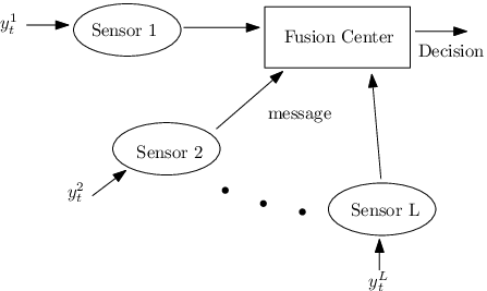
Suppose that $L$ sensors observe samples $y_{t}^{\ell},\;\ell=1,\ldots,L,$ at each discrete time $t$, and communicate to a fusion center which makes the global decision based upon its received messages from sensors, as shown in Fig. 1.

Assuming the existence of density functions, the observed samples are distributed according to $h_{\gamma}(x)$ under the null hypothesis $\mathcal{H}_{0}$ and $f_{\theta}(x)$ under the alternative hypothesis $\mathcal{H}_{1}$. We assume that $\gamma$ and $\theta$ fall within the parameter sets $\Gamma$ and $\Theta$ respectively. Given $\gamma$ and $\theta$, the random samples under both hypotheses are independent over time and across the sensors. Under such a setup, we arrive at a composite null versus composite alternative hypothesis testing problem:

where ${\cal L}\triangleq\{1,\ldots,L\}$. In general, $h_{\gamma}$ and $f_{\theta}$ may belong to different families of distributions. The goal is to find the stopping time $\mathsf{T}$ that indicates the time to stop taking new samples and the decision function $\delta$ that decides between $\mathcal{H}_{0}$ and $\mathcal{H}_{1}$, such that the expected sample size is minimized given the error probabilities are satisfied, i.e.,

where $\mathbb{E}_{\theta}$ denotes expectation taken with respect to (w.r.t.) $f_{\theta}$ and $\mathbb{E}_{\gamma}$ w.r.t. $h_{\gamma}$. Note that (3)-(4) are in fact (possibly uncountably) many optimization problems (depending on the parameter spaces $\Theta$ and $\Gamma$) with the same constraints. Unfortunately, unlike the simple null versus simple alternative hypothesis case, finding a unique optimal sequential test for these problems is infeasible, even when a single-sensor or a centralized setup is considered. Therefore, the approaches that possess asymptotic optimality become the focus of interest. In the following sections, we start by briefly introducing the generalized sequential probability ratio test (GSPRT) as an asymptotically optimal solution for the centralized system; then, two decentralized schemes will be developed based on uniform sampling and level-triggered sampling respectively. In particular, we will show that the latter scheme is asymptotically optimal when certain conditions are met. Here we first give the widely-adopted definition of asymptotic optimality [28, 19].

In this section, we consider the centralized scenario, where local samples $\left\{y_{t}^{\ell}\right\}$ are made available at the fusion center in full precision. Note that the centralized multi-sensor test is not much different from the single-sensor version except that, at each time instant, multiple samples are observed instead of one. Since finding the optimal sequential composite hypothesis testing is impossible, the solutions with asymptotic optimality become the natural alternatives. In particular, the GSPRT is obtained by substituting the unknown parameter with its maximum likelihood estimate in the SPRT; alternatively, one can perform an SPRT using the marginal likelihood ratio by integrating out the unknown parameters when the priors on unknown parameters are available. In this paper, we avoid presuming priors on parameters and adopt the GSPRT.

Due to the conditional independence for samples over time and across sensors, the global likelihood ratio function is evaluated as

Then the centralized GSPRT can be represented with the following stopping time

and the decision function at the stopping instant

Here $\widetilde{S}_{t}$ is referred to as the generalized log-likelihood ratio (GLLR) of the samples up to time $t$, and $A,B$ are prescribed constants such that the error probability constraints in (4) are satisfied. Practitioners can choose their values according to Proposition 1 given below which relates $A,B$ to type-I and type-II error probabilities asymptotically. Before delving into the performance characterization of the centralized GSPRT (7)-(III), we recall the Kullback-Leibler (KL) divergence between two distributions $h_{\gamma}$ and $f_{\theta}$:

Assume that the following conditions/assumptions hold,

• $A1)$

  The distributions under the null and the alternative hypotheses are strictly separated, i.e., $\inf_{\gamma}D\left(f_{\theta}||h_{\gamma}\right)>\varepsilon$ and $\inf_{\theta}D\left(h_{\gamma}||f_{\theta}\right)>\varepsilon$ for some $\varepsilon>0$. This condition implies that the GLLR $\widetilde{S_{t}}$ takes different drifting directions in expectation under the null and the alternative hypotheses ;

• $A2)$

  $D\left(f_{\theta}||h_{\gamma}\right)$ and $D\left(h_{\gamma}||f_{\theta}\right)$ are twice continuously differentiable w.r.t. $\gamma$ and $\theta$;

• $A3)$

  The parameter spaces $\Gamma$ and $\Theta$ are compact sets;

• $A4)$

  Let $S(\gamma,\theta)=\log f_{\theta}(Y)-\log h_{\gamma}(Y)$. There exists $\eta>1,x_{0}$ such that for all $\gamma\in\Gamma,\theta\in\Theta,x>x_{0}$, we have

  		$\displaystyle\mathbb{P}_{\gamma}\left(\sup_{\theta\in\Theta}\left|\nabla_{\theta}S(\gamma,\theta)\right|>x\right)\leq e^{-|\log x|^{\eta}},$		(11)
  	and	$\displaystyle\mathbb{P}_{\theta}\left(\sup_{\gamma\in\Gamma}\left|\nabla_{\gamma}S(\gamma,\theta)\right|>x\right)\leq e^{-|\log x|^{\eta}}.$		(12)

  This condition imposes that the tail of the first-order derivative of the likelihood ratio w.r.t. $\gamma$ or $\theta$ decays faster than any polynomial.

According to [28], the performance of the GSPRT can be characterized asymptotically in closed form, which we quote here as a proposition.

Proposition 1 indicates that the GSPRT, i.e., (7) and (III), is asymptotically optimal among the class of $L$-sensor centralized tests $\mathcal{T}_{c}^{L}(\alpha,\beta)$ in the sense that

as $\alpha\triangleq\sup_{\gamma}\mathbb{P}_{\gamma}\left(\delta_{\mathsf{T}_{c}}=1\right)\to 0$ and $\beta\triangleq\sup_{\theta}\mathbb{P}_{\theta}\left(\delta_{\mathsf{T}_{c}}=0\right)\to 0$ [28, Corollary 2.1]. However, as mentioned in Section I, in spite of its asymptotic optimality, the centralized GSPRT yields substantial data transmission overhead between the sensors and the fusion center; therefore, it may become impractical when the communication resources are constrained. Moreover, the centralized scheme puts all computation burden at the fusion center. Hence, it is of great interest to consider the decentralized scheme where the computation is distributed among the sensors and the fusion center, with much lower communication overhead between the sensors and the fusion center.

In this section, we investigate the decentralized sequential composite hypothesis test, where the fusion center is only able to access a summary of local samples. In particular, each sensor transmits a one-bit message to the fusion center every $T_{0}$ (deterministically or on average) samples. We first consider the conventional decentralized scheme based on the uniform sampling and one-bit quantization. That is, every sensor sends its one-bit quantized local statistic to the fusion center every fixed $T_{0}$ samples. Then we propose a decentralized scheme based on level-triggered sampling (LTS), where the one-bit transmission is stochastically activated by the local statistic process at each sensor, and occurs every $T_{0}$ samples on average. Interestingly, we show that such LTS-based decentralized scheme provably achieves the asymptotic optimality with much lower communication overhead compared with the centralized scheme.

There are a wide range of applications where the decentralized sequential composite hypothesis test plays an important role. In this section, we apply the proposed centralized and decentralized sequential tests to two examples: one is to detect the mean shift of Gaussian random samples; and the other involves spectrum sensing in cognitive radio systems.

References

• [1] H. V. Poor, An Introduction to Signal Detection and Estimation, 2nd ed. New York: Springer, 1994.
• [2] A. Wald and J. Wolfowitz, “Optimum character of the sequential probability ratio test,” The Annals of Mathematical Statistics, vol. 19, no. 3, 1948.
• [3] G. Lorden, “2-SPRT’s and the modified Kiefer-Weiss problem of minimizing an expected sample size,” The Annals of Statistics, vol. 4, no. 2, pp. 281–291, 1976.
• [4] M. Pollak and D. Siegmund, “Approximations to the expected sample size of certain sequential tests,” The Annals of Statistics, vol. 3, no. 6, pp. 1267–1282, 1975.
• [5] T. L. Lai, “Boundary crossing problems for sample means,” Annals of Probability, vol. 28, no. 1, pp. 57–74, 1988.
• [6] T. L. Lai and L. Zhang, “A modification of schwarz’s sequential likelihood ratio tests in multivariate sequential analysis,” Sequential Analysis, vol. 13, no. 2, pp. 79–96, 1994.
• [7] T. L. Lai, “Sequential analysis: Some classical problems and new challenges,” Statistica Sinica, vol. 11, no. 2, pp. 303–408, Apr. 2001.
• [8] I. V. Pavlov, “A sequential procedure for testing many composite hypotheses,” Theory of Probability and its Applications, vol. 21, no. 1, pp. 138–142, 1987.
• [9] ——, “Sequential procedure of testing composite hypotheses with applications to the kiefer-weiss problem,” vol. 35, no. 2, pp. 280–292, 1990.
• [10] V. V. Veeravalli, T. Başar, and H. V. Poor, “Decentralized sequential detection with a fusion center performing the sequential test,” IEEE Trans. Inf. Theory, vol. 39, no. 2, pp. 433–442, Mar. 1993.
• [11] J. N. Tsitsiklis, “Decentralized detection,” Advances in Statistical Signal Processing, vol. 2, pp. 297–344, 1993.
• [12] ——, “On threshold rules in decentralized detection,” in Proc. 25th Conference on Decision and Control, Athens, Greece, Dec. 1986, pp. 232–236.
• [13] X. Nguyen, M. J. Wainwright, and M. I. Jordan, “On optimal quantization rules for sequential decision problems,” in Proc. IEEE Int. Symp. Inf. Theory, Seattle, WA, Jul. 9-14 2006.
• [14] Y. Mei, “Asymptotic optimality theory for decentralized sequential hypothesis testing in sensor networks,” IEEE Trans. Inf. Theory, vol. 54, no. 5, pp. 2072–2089, May 2008.
• [15] Y. Wang and Y. Mei, “Asymptotic optimality theory for decentralized sequential multihypothesis testing problems,” IEEE Trans. Inf. Theory, vol. 57, no. 10, pp. 7068–7083, Oct. 2011.
• [16] ——, “Quantization effect on the log-likelihood ratio and its application to decentralized sequential detection,” IEEE Trans. Signal Process., vol. 61, no. 6, pp. 1536–1543, Mar. 2013.
• [17] V. V. Veeravalli, T. Başar, and H. V. Poor, “Decentralized sequential detection with sensors performing sequential tests,” Mathematics of Control, Signals and Systems, vol. 7, no. 4, pp. 292–305, 1994.
• [18] A. M. Hussain, “Multisensor distributed sequential detection,” IEEE Trans. Aerosp. Electron. Syst., vol. 30, no. 3, pp. 698–708, Jul. 1994.
• [19] G. Fellouris and G. V. Moustakides, “Decentralized sequential hypothesis testing using asynchronous communication,” IEEE Trans. Inf. Theory, vol. 57, no. 1, pp. 534–548, Jan. 2011.
• [20] Y. Yilmaz, G. Moustakides, and X. Wang, “Cooperative sequential spectrum sensing based on level-triggered sampling,” IEEE Trans. Signal Process., vol. 60, no. 9, pp. 4509–4524, Sep. 2012.
• [21] ——, “Channel-aware decentralized detection via level-triggered sampling,” IEEE Trans. Signal Process., vol. 61, no. 2, pp. 300–315, Jan. 2013.
• [22] S. Kar, H. Chen, and P. K. Varshney, “Optimal identical binary quantizer design for distributed estimation,” IEEE Trans. Signal Process., vol. 60, no. 7, pp. 3896–3901, Jul. 2012.
• [23] J. Fang, Y. Liu, H. Li, and S. Li, “One-bit quantizer design for multisensor GLRT fusion,” IEEE Signal Process. Lett., vol. 20, no. 8, Mar. 2013.
• [24] D. Ciuonzo, G. Papa, G. Romano, P. S. Rossi, and P. Willett, “One-bit decentralized detection with a Rao test for multisensor fusion,” IEEE Signal Process. Lett., vol. 20, no. 9, pp. 861–864, Sep. 2013.
• [25] A. G. Tartakovsky and A. S. Polunchenko, “Quickest changepoint detection in distributed multisensor systems under unknown parameters,” in Proc. 11th International Conference on Information Fusion, Cologne, Germany, 30 June-3 July 2008.
• [26] S. Li and X. Wang, “Quickest attack detection in multi-agent reputation systems,” IEEE J. Sel. Topics Signal Process., vol. 8, no. 4, pp. 653–666, Aug. 2014.
• [27] S. Li, Y. Yılmaz, and X. Wang, “Quickest detection of false data injection attack in wide-area smart grid,” IEEE Trans. Smart Grid, to appear. [Online]. Available: 10.1109/TSG.2014.2374577.
• [28] X. Li, J. Liu, and Z. Ying, “Generalized sequential probability ratio test for separate families of hypotheses,” Sequential Analysis, vol. 33, no. 4, pp. 539–563, Oct. 2014.
• [29] R. S. Blum, S. A. Kassam, and H. V. Poor, “Distributed detection with multiple sensors: Part II–advanced topics,” Proceedings of IEEE, vol. 85, no. 1, pp. 64–79, Jan. 1997.
• [30] J. N. Tsitsiklis, “Extremal properties of likelihood ratio quantizers,” IEEE Trans. Commun., vol. 41, no. 4, pp. 550–558, 1993.
• [31] J. Font-Segura and X. Wang, “GLRT-Based Spectrum Sensing for Cognitive Radio with Prior Information,” IEEE Trans. Commun., vol. 58, no. 7, pp. 2137–2146, Jul. 2010.
• [32] H. Chernoff, “A measure of asymptotic efficiency for tests of a hypothesis based on the sum of observations,” The Annals of Mathematical Statistics, pp. 493–507, 1952.