Wave-Packet Analysis of Single-Slit Ghost Diffraction
Abstract
We show that single-slit two-photon ghost diffraction can be explained very simply by using a wave-packet evolution of a generalised EPR state. Diffraction of a wave travelling in the x-direction can be described in terms of the spreading in time of the transverse (z-direction) wave-packet, within the Fresnel approximation. The slit is assumed to truncate the transverse part of the wavefunction of the photon to within the width of the slit. The analysis reproduces all features of the two-photon single-slit ghost diffraction.
pacs
03.65.Ud and 03.65.Ta1 Introduction
The issue of quantum nonlocality which results from entangled states, has been a subject of debate since the time it was brought to prominence by the seminal paper of Einstein, Podolsky and Rosen (EPR)[1]. Quantum systems which are said to be entangled, show certain correlation in their measurement results even though they may be far separated in space,[2]. This is a feature of quantum mechanics which many find discomforting.
A dramatic demonstration of quantum nonlocality is in the so-called ghost interference experiment by Strekalov et.al.[3]. We describe below, the single-slit ghost diffraction experiment.
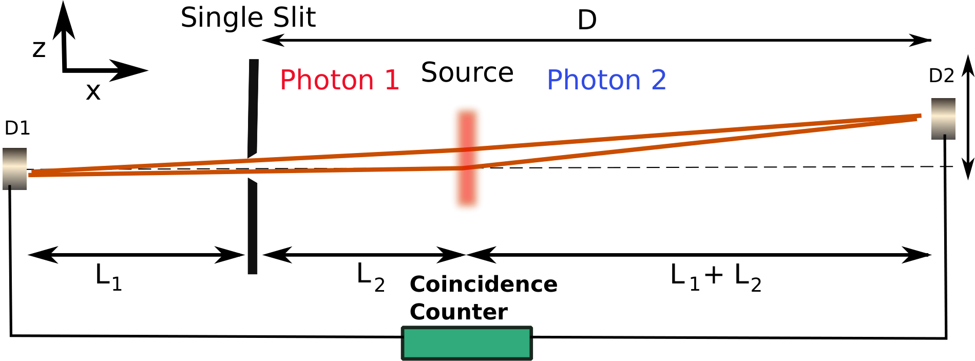
An entangled pair of photons emerges from a spontaneous parametric down-conversion (SPDC) source S. Photons, which we shall refer to as 1 and 2, are separated by a beam-splitter and travel in different directions, A single-slit is kept in the path of photon 1, and there is a movable detector D1 behind it (see Fig. 1). Normally one would expect a single-slit diffraction pattern. No first order diffraction is observed for photon 1. This result is unexpected because one would expect photons from a laser, passing through a single-slit, to undergo diffraction. The second, and the more surprising result of the experiment is that when photon 2 is detected by detector D2, in coincidence with a fixed detector D1 detecting photon 1, photon 2 shows a single-slit diffraction pattern. Photon 2 does not pass through any slit, and one would not expect it to show any diffraction. Another curious feature of this ghost-diffraction is that the fringe width of the diffraction pattern follows a diffraction formula , where is the wavelength of the photons, the width of the slit, and is a very curious distance from slit, right through the SPDC source to the detector D2. Note that photon 2 does not even travel that much of distance. The experiment attracted a lot of debate and research attention [4, 5, 6, 7, 8, 9, 10, 11, 12].
The double-slit version of this experiment has been understood as a combined effect of a virtual double-slit creation for photon 2, and quantum erasure of which-path information[10, 11, 12]. In that analysis the amplitudes of photon 1, to pass through the two slits, are correlated with certain amplitudes of photon 2. However, the correlation between the two photons within the narrow region of one slit had been ignored. In order to explain single-slit ghost diffraction, one would need to take into account the entanglement between the photons within the region of a single slit. A rigorous theoretical analysis of the single-slit ghost experiment would involve introducing a two-photon entangled state, and evolving it in time in the presence of single-slit potential. This is a challenging task.
It has been shown earlier that diffraction of light can be described in terms of evolution of de Broglie wave-packets[13, 14]. Single-slit diffraction of light in particular, has been described in terms of Gaussian wave-packet evolving via Schrödinger evolution[15]. In the following we generalise these methods to the case of an entangled state. We show that the single-slit ghost diffraction can be explained rather simply using this approach.
2 Wave-packet analysis
2.1 The entangled state
We start with a generalised EPR state[16]
| (1) |
where is a normalization constant, and are certain parameters to be explained later. The state (1), unlike the original EPR state[1], is well behaved and fully normalised. In the limit the state (1) reduces to the original EPR state.
The photons of the pair are assumed to be travelling in opposite directions along the x-axis, but the entanglement is in the z-direction. In our analysis we will ignore the dynamics along the x-axis as it does not affect the entanglement. We just assume that during evolution for a time , the photon travels a distance equal to in the x-direction. Integration over can be performed in (1) to obtain:
| (2) |
The uncertainty in position and the wave-vector of the two photons, along the z-axis, is given by
| (3) |
From the above it is clear that and quantify the position and momentum (wave-vector) spread of the photons in the z-direction. Notice however, that for the special case , the state (2) is factored into a product of two Gaussians for and alone. Thus the state is not entangled for this particular choice of parameters.
2.2 Time evolution
We first lay out our strategy for the time evolution of a photon wave-packet. Consider the state of a single photon at time as . The state at a later time is given by
| (4) |
where is the Fourier transform of with respect to . Now photon is approximately travelling in the x-direction, but can slightly deviate in the z-direction (which allows it to pass through slits located at different z-positions), so that its true wave-vector will have a small component in the z-direction too. So
| (5) |
Since the photon is travelling along x-axis by and large, we can write , where is the wavenumber of the photon associated with its wavelength, . The dispersion along z-axis can then be approximated by
| (6) |
This is essentially the Fresnel approximation. Using this approximation, eqn. (4) assumes the form
| (7) |
Coming back to our problem of entangled photons, we assume that after travelling for a time , photon 1 reaches the slit (), and photon 2 travels a distance towards detector D2. Using the strategy outlined in the preceding discussion, we can write the state of the entangled photons after a time as follows:
| (8) |
where is the Fourier transform of (2) with respect to . After some algebra, the above can be worked out to be
| (9) |
where . The above equation represents the state of the entangled photons just before photon 1 enters the slit.
2.3 Effect of slit
In order to incorporate the effect of the slit of width on the entangled state, we just assume that the slit abruptly truncates the state of particle 1 such that only the part survives. Consequently we assume this truncated state to be our starting point after emerging from the slit. After emerging from the slit, photon 1 travels for a time , a distance , to reach the detector D1, and photon 2 travels for the same time to reach detector D2. Using (7), the time propagation kernel for the two photons can be written as
| (10) |
The two-particle state after a time (after ) is given by
| (11) |
Notice that because of the truncation, the wavefunction above is no longer normalised. Subsequently we will continue to treat the unnormalised wavefunction. Integration over can be performed straightaway to give
| (12) |
where
| (13) |
and .
Assuming the slit is very narrow, we notice that in the integral above, . Hence we can make the following approximation
| (14) |
where is or . This amounts to neglecting in comparison to , and results in
| (15) |
In (12), the argument of the exponent in the last term is of the order of , and thus that term has been neglected in writing the above approximate form.
Integration over can now be carried out with ease, and one obtains
| (16) |
where and .
The probability density of joint detection of photon 2 at , and photon 1 at , is given by
| (17) |
Before we come to the results, we recall that the final expression is understood better in terms of the distance travelled by the photons, rather than the time for which they evolve. In the following analysis, we use and .
3 Results
3.1 Ghost diffraction
Ghost diffraction arises when photon 2 is detected at D2 in coincidence with photon 1 being detected at D1 fixed at . The probability density of this happening can be evaluated by putting in (17). Entanglement between the two photons is good when . In this limit we safely assume . In the approximation , this (unnormalised) probability density assumes the form
| (18) |
where
| (19) |
Squares represent the experimental data from Strekalov et. al. [3].
The probability density, given by (18), represents a diffraction pattern for photon 2. In order to compare the theoretical results obtained here with the experimental results of Strekalov et.al., (18) has been plotted after normalising and scaling with 500 counts, and using the other parameter values of the experiment (see Fig. 2). The parameter has been assigned an arbitrary value 5 mm-1. The name ghost diffraction is natural for this phenomenon, as photon 2 does not pass through any real slit, but still shows diffraction. The distance between the central maximum and the first maximum is given by
| (20) |
The surprise here is that, taken at face value, the above formula would represent diffraction of photons of wavelength emerging from a slit of width and travelling a distance to reach detector D2. However, photons 2 really travel only a distance . This is exactly what was seen in the experiment [3]. This quaint feature is the result of entanglement between the two photons.
As a special case, if we find that and consequently . In the limit , the pobability density of detecting photon 2 at a position , in coincidence with D1 fixed at , is given by
| (21) |
This is just a Gaussian in and implies that there is no ghost diffraction, which should not be surprising because for the two photons are disentangled.
Let us try to understand why a coincident count of D2 with a fixed D1 is needed for ghost interference to appear. Not doing a coincident count would amount to integrating over , the position of D2, in (17). It can be easily seen that, for , integration over would kill the oscillations in (17), which means no ghost diffraction.
Another way to understand why coincident counting is needed for ghost diffraction is that if D1 were fixed at instead of , the term would lead to a slightly shifted ghost diffraction pattern. This feature has also been experimentally observed [3]. Corresponding to different values of , the diffraction pattern would be shifted by different amounts, and a sum of all such possibilities would lead to the washing out of the pattern.
3.2 Missing first order diffraction
Let us now turn our attention to the issue of missing first order single-slit diffraction for photon 1 behind the slit. In the first part of the experiment, photons 1 pass through the single slit and are detected by a scanning detector D1. Normally one would expect single slit diffraction. The authors of the experiment explain it by saying that the blurring out of the first order interference fringes is due to the considerably large angular propagation uncertainty of a single SPDC photon. However, we will show that the real reason lies in the entanglement of photon 1 with photon 2.
The probability of joint detecttion of the two photons at the two detectors is given by (17). If one wants to look for first order diffraction of photon 1, one has to ignore photon 2 or, in other words, integrate over all values of . Clearly, if one were to evaluate using (17), the oscillations will be gone and it will not yield a diffraction pattern. Interestingly however, for the case (), (17) reduces to
| (22) |
The above represents a diffraction pattern for photon 1 without any coincident counting, since integration over does not effect the dependent terms. It also says that photon 2 has a Gaussian distribution. As expected, if the two photons are not entangled, first order diffraction will be visible for photon 1, and photon 2 will not show any ghost diffraction. For , entanglement will kill any first order diffraction.
Another way to understand the missing first order interference is that by virtue of entanglement, each path of the photon 1, within the width of the slit, is correlated with a particular path of of photon 2. By measuring the position of photon 2, one can, in principle, find out which particular path photon 1 had taken. If which-path information exists, no interference between different paths is possible, by virtue of Bohr’s complementarity principle [17].
4 Conclusion
We have theoretically analysed the single-slit ghost diffraction experiment with entangled photons by using Fourier wave-packet evolution. At the heart of analysis is a generalised EPR state which describes the entangled photons. The effect of the slit is assumed to be a truncation of the wavefunction of the photon to within the width of the slit. Subsequent evolution is free. This simple analysis quantitatively reproduces all features of single-slit ghost diffraction. It explains why the diffraction pattern shifts if the detector D1 is fixed at a location other than . It explains the strange distance that appears in the fringe-width formula of the ghost diffraction, eventhough the photon never actually travels that distance. This analysis also explains why first order diffraction behind the single slit is not observed.
Acknowledgements.
Sheeba Shafaq thanks the Centre for Theoretical Physics, JMI, for providing her the facilities of the centre during the course of this work.References
- (1) A. Einstein, B. Podolsky, N. Rosen, Can quantum-mechanical description of physical reality be considered complete? Phys. Rev. 47 (1935) 777–780.
- (2) E. Schrödinger, Discussion of probability relations between separated systems, Math. Proc. Cambridge Philos. Soc., 31 (1935) 555–563.
- (3) D.V. Strekalov, A.V. Sergienko, D.N. Klyshko, Y.H. Shih, Observation of two-photon ghost interference and diffraction, Phys. Rev. Lett. 74 (1995) 3600.
- (4) M. D’Angelo, Y-H. Kim, S. P. Kulik and Y. Shih, Phys. Rev. Lett. 92, 233601 (2004).
- (5) S. Thanvanthri and M. H. Rubin, Phys. Rev. A 70, 063811 (2004).
- (6) Y-H. Zhai, X-H. Chen, D. Zhang, L-A. Wu, Phys. Rev. A 72, 043805. (2005).
- (7) L. Jie, C. Jing, Chinese Phys. Lett. 28, 094203 (2011).
- (8) J. Kofler, M. Singh, M. Ebner, M. Keller, M. Kotyrba, A. Zeilinger, Phys. Rev. A 86, 032115 (2012).
- (9) D-S. Ding, Z-Y. Zhou, B-S. Shi, X-B Zou, G-C. Guo, AIP Advances 2, 032177 (2012).
- (10) P. Chingangbam, T. Qureshi, Prog. Theor. Phys. 127, 383-392 (2012).
- (11) S. Shafaq, T. Qureshi, Eur. Phys. J. D 68, 52 (2014).
- (12) T. Qureshi, P. Chingangbam, S. Shafaq, “Understanding ghost interference,” arXiv:1406.0633 [quant-ph]
- (13) G. Vandegrift, “The diffraction and spreading of a wavepacket,” Am. J. Phys. 72, 404 (2004).
- (14) G. Dillon, “Fourier optics and time evolution of de Broglie wave packets,” Eur. Phys. J. Plus 127, 66 (2012).
- (15) A. Zecca, “Diffraction of Gaussian wave packets by a single slit,” Eur. Phys. J. Plus 126, 18 (2011).
- (16) T. Qureshi, “Understanding Popper’s experiment,” Am. J. Phys. 73, 541 (2005).
- (17) N. Bohr, Nature 121 (1928), 580.