跳到论文正文
W Papers独立论文阅读器 arXiv:1505.05313 论文正文 计算阅读时间 · 0%
引用这篇论文根据当前论文元数据生成,正式投稿前建议核对。


License: arXiv.org perpetual non-exclusive license
arXiv:1505.05313v1 [math.AP] 20 May 2015

Emergence of Unstable Modes
for Shock Waves in Ideal MHD

Heinrich Freistühler11 1 Department of Mathematics, University of Konstanz, 78457 Konstanz, Germany    Felix Kleber11 1 Department of Mathematics, University of Konstanz, 78457 Konstanz, Germany    and Johannes Schropp11 1 Department of Mathematics, University of Konstanz, 78457 Konstanz, Germany
Abstract

This note studies classical magnetohydrodynamic shock waves in an inviscid fluidic plasma that is assumed to be a perfect conductor of heat as well as of electricity. For this mathematically prototypical material, it identifies a critical manifold in parameter space, across which slow classical MHD shock waves undergo emergence of a complex conjugate pair of unstable transverse modes. In the reflectionally symmetric case of parallel shocks, this emergence happens at the spectral value λ^≡λ/|ω|=0\hat{\lambda}\equiv\lambda/|\omega|=0, and the critical manifold possesses a simple explicit algebraic representation. Results of refined numerical treatment show that for only almost parallel shocks the unstable mode pair emerges from two spectral values λ^=±i​γ,γ>0\hat{\lambda}=\pm i\gamma,\gamma>0.

1 The equations of ideal isothermal MHD

We consider ideal MHD in twodimensional space,

0=\displaystyle 0= ρt+div​(ρ​V)\displaystyle\rho_{t}+\text{div}(\rho V) (1)
0=\displaystyle 0= (ρ​V)t+div​(ρ​V⊗V+(p+12​|B|2)​I−B⊗B)\displaystyle(\rho V)_{t}+\text{div}(\rho V\otimes V+(p+\frac{1}{2}|B|^{2})I-B\otimes B)
0=\displaystyle 0= Bt+div​(B⊗V−V⊗B).\displaystyle B_{t}+\text{div}(B\otimes V-V\otimes B).

The dependent variables ρ>0,p>0,V∈ℝ2\rho>0,p>0,V\in\mathbb{R}^{2} denote the fluid’s density, pressure, and velocity. In addition to (1), the magnetic field B∈ℝ2B\in\mathbb{R}^{2} satisfies

div​B=0.\text{div}\,B=0. (2)

The fluid is assumed to be polytropic, p=R​ρ​Tp=R\rho T, and have a constant temperature TT, so that p=c2​ρp=c^{2}\rho with constant sound speed cc. By scaling, we assume without loss of generality that

p=ρ,i. e., the speed of sound is ​1.p=\rho,\quad\text{i.\ e., the speed of sound is }1. (3)

We abbreviate (1) as

Ut+F​(U)x+G​(U)y=0U_{t}+F(U)_{x}+G(U)_{y}=0 (4)

with

U=(ρρ​v1ρ​v2b1b2),F⁡(U)=(ρ​v1ρ​v1​v1+p+12​(b22−b12)ρ​v1​v2−b1​b20b2​v1−v2​b1),G⁡(U)=(ρ​v2ρ​v2​v1−b2​b1ρ​v2​v2+p+12​(b12−b22)b1​v2−v1​b20).U=\begin{pmatrix}\rho\\ \rho v_{1}\\ \rho v_{2}\\ b_{1}\\ b_{2}\end{pmatrix},\quad F(U)=\begin{pmatrix}\rho v_{1}\\ \rho v_{1}v_{1}+p+\frac{1}{2}(b_{2}^{2}-b_{1}^{2})\\ \rho v_{1}v_{2}-b_{1}b_{2}\\ 0\\ b_{2}v_{1}-v_{2}b_{1}\end{pmatrix},\quad G(U)=\begin{pmatrix}\rho v_{2}\\ \rho v_{2}v_{1}-b_{2}b_{1}\\ \rho v_{2}v_{2}+p+\frac{1}{2}(b_{1}^{2}-b_{2}^{2})\\ b_{1}v_{2}-v_{1}b_{2}\\ 0\end{pmatrix}.

Using (2), we also write it as a symmetric hyperbolic system11 1 This issue has an interesting history, cf. [9, 6].,

𝐃⁡(U~)​U~t+𝐀~​(U~)​U~x+𝐁~​(U~)​U~y=0{\bf D}(\tilde{U})\tilde{U}_{t}+\tilde{\bf A}(\tilde{U})\tilde{U}_{x}+\tilde{\bf B}(\tilde{U})\tilde{U}_{y}=0 (5)

with U~=(ρ,v1,v2,b1,b2)⊤\tilde{U}=(\rho,v_{1},v_{2},b_{1},b_{2})^{\top}, 𝐃⁡(U~)=diag​(1/ρ,ρ,ρ,1,1){\bf D}(\tilde{U})=\text{diag}(1/\rho,\rho,\rho,1,1), and

𝐀~​(U~)=(v1/ρ10001ρ​v100b200ρ​v10−b1000v100b2−b10v1),𝐁~​(U~)=(v2/ρ01000ρ​v20−b2010ρ​v2b100−b2b1v200000v2).\tilde{\bf A}(\tilde{U})=\begin{pmatrix}v_{1}/\rho&1&0&0&0\\ 1&\rho v_{1}&0&0&b_{2}\\ 0&0&\rho v_{1}&0&-b_{1}\\ 0&0&0&v_{1}&0\\ 0&b_{2}&-b_{1}&0&v_{1}\end{pmatrix},\quad\tilde{\bf B}(\tilde{U})=\begin{pmatrix}v_{2}/\rho&0&1&0&0\\ 0&\rho v_{2}&0&-b_{2}&0\\ 1&0&\rho v_{2}&b_{1}&0\\ 0&-b_{2}&b_{1}&v_{2}&0\\ 0&0&0&0&v_{2}\end{pmatrix}.

Applying the chain rule, we rewrite (5) as

Ut+𝐀⁡(U)​Ux+𝐁⁡(U)​Uy=0,U_{t}+{\bf A}(U)U_{x}+{\bf B}(U)U_{y}=0, (6)

where

𝐀=𝐓𝐃−1​𝐀~​𝐓−1,𝐁=𝐓𝐃−1​𝐁~​𝐓−1{\bf A}={\bf T}{\bf D}^{-1}\tilde{{\bf A}}{\bf T}^{-1},\quad{\bf B}={\bf T}{\bf D}^{-1}\tilde{{\bf B}}{\bf T}^{-1} (7)

with

𝐓=∂U∂U~=(100Vρ​I2000I2).{\bf T}=\frac{\partial U}{\partial\tilde{U}}=\begin{pmatrix}1&0&0\\ V&\rho I_{2}&0\\ 0&0&I_{2}\end{pmatrix}. (8)

Note that, as we have used (2) on the way from (1) to (5), the matrices 𝐀\bf A and 𝐁\bf B in (6) are not the Jacobians of the fluxes FF and GG.

2 Slow and fast, parallel and non-parallel shock waves

Ideal MHD shock waves, in their prototypical form, have the structure

U⁡(t,x,y)={U−=(ρ−,ρ−​V−,H−),(x,y)⋅N<s​t,U+=(ρ+,ρ+​V+,H+),(x,y)⋅N>s​t,U(t,x,y)=\begin{cases}U^{-}=(\rho^{-},\rho^{-}V^{-},H^{-}),&(x,y)\cdot N<st,\\ U^{+}=(\rho^{+},\rho^{+}V^{+},H^{+}),&(x,y)\cdot N>st,\end{cases}

where N=(N1,N2)∈S1N=(N_{1},N_{2})\in S^{1} is the direction of propagation and ss the speed of the shock wave. Function (9) being a weak solution of (1) is equivalent to the Rankine-Hugoniot conditions

−s⁡(U+−U−)+N1​(F⁡(U+)−F⁡(U−))+N2​(G⁡(U+)−G⁡(U−))=0.-s(U^{+}-U^{-})+N_{1}(F(U^{+})-F(U^{-}))+N_{2}(G(U^{+})-G(U^{-}))=0.

Due to rotational and Galilean invariance it is without loss of generality that we henceforth assume that

N=(1,0)ands=0;N=(1,0)\quad\text{and}\quad s=0;

i. e. we exclusively consider shock waves of the form

U⁡(t,x,y)={U−=(ρ−,ρ−​V−,H−),x<0,U+=(ρ+,ρ+​V+,H+),x>0,U(t,x,y)=\begin{cases}U^{-}=(\rho^{-},\rho^{-}V^{-},H^{-}),&x<0,\\ U^{+}=(\rho^{+},\rho^{+}V^{+},H^{+}),&x>0,\end{cases} (9)

and the Rankine-Hugoniot conditions read

F⁡(U−)=F⁡(U+).F(U^{-})=F(U^{+}). (10)

Note now first that for waves (9), as for any solutions of (1) whose spatial dependence is only via xx, the divergence-free condition (2) reduces to

b1=a,a​ any constant.b_{1}=a,\quad a\text{ any constant.} (11)

We assume (11) and simply write b,v,wb,v,w instead of b2,v1,v2b_{2},v_{1},v_{2}.

In this paper, we are interested in Lax shocks. Following [8, 1, 3, 4], two states

U−=(ρ−,ρ−​v−,ρ−​w−,a,b−)andU+=(ρ+,ρ+​v+,ρ+​w+,a,b+)U^{-}=(\rho^{-},\rho^{-}v^{-},\rho^{-}w^{-},a,b^{-})\quad\text{and}\quad U^{+}=(\rho^{+},\rho^{+}v^{+},\rho^{+}w^{+},a,b^{+}) (12)

that satisfy the Rankine-Hugoniot conditions (10) constitute a

slow Lax shock iff ​0<ρ+​(v+)2<ρ−​(v−)2<a2\text{slow Lax shock iff }0<\rho^{+}(v^{+})^{2}<\rho^{-}(v^{-})^{2}<a^{2} (13)

and a

fast Lax shock iff ​a2<ρ​(v+)2<ρ−​(v−)2.\text{fast Lax shock iff }a^{2}<\rho(v^{+})^{2}<\rho^{-}(v^{-})^{2}. (14)

Two states (12) do satisfy the Rankine-Hugoniot conditions (10) if and only if the two quadruples (ρ−,v−,w−,b−)(\rho^{-},v^{-},w^{-},b^{-}) and (ρ+,v+,w+,b+)(\rho^{+},v^{+},w^{+},b^{+}) have coinciding images under the mapping

(ρvwb)↦(ρ​vρ​v2+ρ+12​b2ρ​v​w−a​bb​v−a​w)\begin{pmatrix}\rho\\ v\\ w\\ b\end{pmatrix}\mapsto\begin{pmatrix}\rho v\\ \rho v^{2}+\rho+\frac{1}{2}b^{2}\\ \rho vw-ab\\ bv-aw\end{pmatrix} (15)

that FF induces by omitting its forth, trivial component, in other words if both quadruples satisfy the four equations

ρ​v\displaystyle\rho v =\displaystyle= m\displaystyle m (16)
ρ​v2+ρ+12​b2\displaystyle\rho v^{2}+\rho+\frac{1}{2}b^{2} =\displaystyle= j\displaystyle j (17)
v​b−a​w\displaystyle vb-aw =\displaystyle= c\displaystyle c (18)
m​w−a​b\displaystyle mw-ab =\displaystyle= d\displaystyle d (19)

for the same values of the four parameters m,j,c,d∈ℝm,j,c,d\in\mathbb{R}. As simple arguments22 2 reversing, shifting, scaling, and the observation that cases with m=0m=0 or ρ​v2=a2\rho v^{2}=a^{2} give no Lax shocks show, we lose no generality in assuming that

m>0,d=0,and ​ρ​v2≠a2.m>0,\quad d=0,\quad\text{and }\rho v^{2}\neq a^{2}. (20)

Using (19) in (18) and inserting the result and (16) in (17) then yields

ga​m​c​(v)≡m​1+v2v+12​(m​cm​v−a2)2=j,to be solved for ​v∈(0,a2/m)∪(a2/m,∞).g^{amc}(v)\equiv m\frac{1+v^{2}}{v}+\frac{1}{2}\bigg(\frac{mc}{mv-a^{2}}\bigg)^{2}=j,\ \ \hbox{to be solved for }v\in(0,a^{2}/m)\cup(a^{2}/m,\infty). (21)

As for every solution vv of (21), relations (16), (18), (19) provide unique associated values for v,wv,w and bb, understanding (21) will give a complete picture. One distinguishes two cases.

c=0c=0: parallel shocks. In this case, (21) has two solutions

v±=12​(jm∓(jm)2−4)if ​jm>2,with ​0<v+<v−.v^{\pm}=\frac{1}{2}\bigg(\frac{j}{m}\mp\sqrt{\big(\frac{j}{m}\big)^{2}-4}\bigg)\quad\text{if }\frac{j}{m}>2,\quad\text{with }0<v^{+}<v^{-}.

The corresponding states (12) constitute a

slow parallel shock iff ​m​v−<a2\text{slow parallel shock iff }mv^{-}<a^{2} (22)

and a

fast parallel shock iff ​a2<m​v+.\text{fast parallel shock iff }a^{2}<mv^{+}. (23)

The fact that the value of aa has no influence on the ρ,v,w,b\rho,v,w,b components of parallel shocks is easily understood by noticing that they have b=w=0b=w=0 and thus are purely gas dynamical.

c≠0c\neq 0: non-parallel shocks. In this case, ga​m​cg^{amc} tends to ∞\infty not only for v↘0v\searrow 0 und v↗∞v\nearrow\infty, but also for v→a2/mv\to a^{2}/m. Thus for every

j>jm​i​ns​(a,m,c)=min(0,a2/m)⁡ga​m​c,j>j^{s}_{min}(a,m,c)=\min_{(0,a^{2}/m)}g^{amc},

(21) has two solutions

vs+​(a,m,c,j)<vs−​(a,m,c,j)<a2/mv^{+}_{s}(a,m,c,j)<v^{-}_{s}(a,m,c,j)<a^{2}/m

that consitute a slow shock. Similarly, for every

j>jm​i​nf​(a,m,c)=min(a2/m,∞)⁡ga​m​c,j>j^{f}_{min}(a,m,c)=\min_{(a^{2}/m,\infty)}g^{amc},

there are two solutions

a2/m<vf+​(a,m,c,j)<vf−​(a,m,c,j)a^{2}/m<v^{+}_{f}(a,m,c,j)<v^{-}_{f}(a,m,c,j)

that define a fast shock.

3 Lopatinski determinant and critical manifold

According to Majda’s theory33 3 This is what our passing, in Sec. 1, through the symmetric hyperbolic formulation (5) is needed for. [10, 11] on the persistence of shock fronts, the local-in-time stability of the planar discontinous wave (9) is determined by the behaviour of the Lopatinski determinant

Δ:S+=(ℂ+¯×ℝ)∖{(0,0)}→ℂ,Δ⁡(λ,ω):=det(R−​(λ,ω),J⁡(λ,ω),R+​(λ,ω)),\Delta:S_{+}=(\overline{\mathbb{C}_{+}}\times\mathbb{R})\setminus\{(0,0)\}\to\mathbb{C},\quad\Delta(\lambda,\omega):=\det(R^{-}(\lambda,\omega),J(\lambda,\omega),R^{+}(\lambda,\omega)), (24)

where ℂ+={λ∈ℂ:ℜ⁡λ>0}\mathbb{C}_{+}=\{\lambda\in\mathbb{C}:\Re\lambda>0\}. While uniform stability corresponds to the non-vanishing of Δ\Delta on all of S+S_{+}, shocks with

∅≠Δ−1​(0)⊂i​ℝ×ℝor∅≠Δ−1​(0)∩(ℂ+×ℝ)\emptyset\neq\Delta^{-1}(0)\subset i\mathbb{R}\times\mathbb{R}\qquad\text{or}\qquad\emptyset\neq\Delta^{-1}(0)\cap(\mathbb{C}_{+}\times\mathbb{R}) (25)

are neutrally stable or strongly unstable, respectively. The ingredients of the Lopatinski determinant are

J⁡(λ,ω):=λ⁡(U+−U−)+i​ω​(G⁡(U+)−G⁡(U−)),“jump vector”,\displaystyle J(\lambda,\omega):=\lambda(U^{+}-U^{-})+i\omega(G(U^{+})-G(U^{-})),\text{``jump vector''},
R−​(λ,ω), base of the stable space of ​𝐋−:=(λ​𝐈+i​ω​𝐁−)​(𝐀−)−1,\displaystyle R^{-}(\lambda,\omega),\text{ base of the stable space of }{\bf L}^{-}:=(\lambda{\bf I}+i\omega{\bf B}^{-})({\bf A}^{-})^{-1},
R+​(λ,ω), base of the unstable space of ​𝐋+:=(λ​𝐈+i​ω​𝐁+)​(𝐀+)−1,\displaystyle R^{+}(\lambda,\omega),\text{ base of the unstable space of }{\bf L}^{+}:=(\lambda{\bf I}+i\omega{\bf B}^{+})({\bf A}^{+})^{-1},

where 𝐀±,𝐁±{\bf A}^{\pm},{\bf B}^{\pm} denote 𝐀⁡(U±),𝐁⁡(U±){\bf A}(U^{\pm}),{\bf B}(U^{\pm}). The theory of hyperbolic initial-boundary value problems [7, 10] implies that R±R^{\pm} are well-defined bundles of constant dimension. To be precise, it is on ℂ+×ℝ=S+∖(i​ℝ×ℝ)\mathbb{C}_{+}\times\mathbb{R}=S_{+}\setminus(i\mathbb{R}\times\mathbb{R}) that the Lopatinski matrices 𝐋±{\bf L}^{\pm} have constantly trivial neutral spaces and thus “consistent splitting”, i. e., stable and unstable spaces of constant dimensions, so that in particular

d−=dimspan ​R−​(λ,ω)andd+=dimspan ​R+​(λ,ω)d^{-}=\dim\text{span }R^{-}(\lambda,\omega)\quad\text{and}\quad d^{+}=\dim\text{span }R^{+}(\lambda,\omega)

are constant; for points (λ,ω)∈S+(\lambda,\omega)\in S_{+} with purely imaginary values of λ\lambda, the R±​(λ,ω)R^{\pm}(\lambda,\omega) are defined as limits from the interior of S+S_{+} [7]. From the one-dimensional ‘Lax counting’ of characteristic speeds [8, 1], we know that

d−=1andd+=3for slow MHD shocks,d^{-}=1\quad\text{and}\quad d^{+}=3\quad\text{for slow MHD shocks}, (26)

while

d−=0andd+=4for fast MHD shocks.d^{-}=0\quad\text{and}\quad d^{+}=4\quad\text{for fast MHD shocks}. (27)

The Lopatinski determinant Δ\Delta being degree-one homogeneous in (λ,ω)(\lambda,\omega), we from now on fix the transverse wave number to

ω=±1.\omega=\pm 1.

To avoid abundant notation, we also fix from now, again without loss of generality,

ρ−=1\rho^{-}=1 (28)

and use the two parameters ρ+,c\rho^{+},c instead of the three paramters j,m,cj,m,c. For parallel shocks, our choice (28) implies

v−=ρ+,v+=1/ρ+.v^{-}=\sqrt{\rho^{+}},\quad v^{+}=1/\sqrt{\rho^{+}}.

In this paper we concentrate on slow shocks.44 4 Cf. Trakhinin’s paper [12] (and also [2, 5]) for other results. The following is a key observation.

Theorem 1.

For slow parallel MHD shocks in (1),(2) with (3) and ρ−=1\rho^{-}=1,

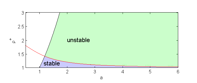
Δ⁡(0,±1)=0ifρ+=a2+2a2+1.\Delta(0,\pm 1)=0\quad\text{if}\quad{\rho^{+}}=\frac{a^{2}+2}{a^{2}+1}. (29)
Proof.

Interesting manipulations show that one can take

R−=(1ρ+−i​(a2−ρ+)​(a2ρ+−11−ρ+)a0),R+=(ρ+a⁡(ρ+−1)020000−a​ρ+020001).R^{-}=\begin{pmatrix}1\\ \sqrt{\rho^{+}}\\ -i\sqrt{\bigg({a^{2}-\rho^{+}}\bigg)\bigg(\frac{a^{2}}{\rho^{+}}-\frac{1}{1-\rho^{+}}\bigg)}\\ a\\ 0\end{pmatrix},\quad R^{+}=\begin{pmatrix}\sqrt{\rho^{+}}&a(\rho^{+}-1)&0\\ 2&0&0\\ 0&0&-a\sqrt{\rho^{+}}\\ 0&2&0\\ 0&0&1\end{pmatrix}.

Together with J=(0,0,i,0,0)J=(0,0,i,0,0), this yields

Δ⁡(0,1)=2​i​[ρ+​(a2+1)−(a2+2)].\Delta(0,1)=2i[\rho^{+}(a^{2}+1)-(a^{2}+2)].

∎

Refer to caption
Figure 1: Slow parallel shock with ρ−=1\rho^{-}=1, cf. Theorem 1. The black boundary is the Lax condition (22): ρ−​(v−)2<a2\rho^{-}(v^{-})^{2}<a^{2}.

4 Symmetry breaking

The situation of parallel shocks is degenerate as it possesses a reflectional symmetry in the transverse (yy-)direction. For the Lopatinski determinant this symmetry means that Δ⁡(λ,−ω)\Delta(\lambda,-\omega) vanishes exactly if Δ⁡(λ,ω)\Delta(\lambda,\omega) does. Perturbing the parameter cc away from 00 breaks this symmetry, and the zero of Δ\Delta that we found, for c=0c=0 at λ=0\lambda=0, splits.

For all values of ρ+,a,c\rho^{+},a,c that permit a (then unique) slow MHD shock wave, we write Δρ+,a,c\Delta^{\rho^{+},a,c} for the corresponding Lopatinski determinant. Starting from Theorem 1, we found the following.

Numerical Observation 1.

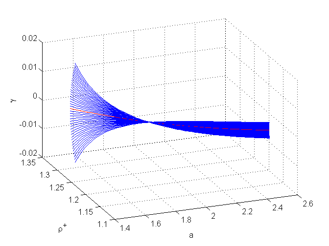
There are an ϵ>0\epsilon>0 and two functions,

R⁡(a,c),even in ​c​ and with ​R​(a,0)=a2+2a2+1,andγ⁡(a,c),odd in ​c,R(a,c),\text{even in }c\text{ and with }R(a,0)=\frac{a^{2}+2}{a^{2}+1},\quad\text{and}\quad\gamma(a,c),\text{odd in }c,

both defined on Ωϵ={(a,c):a≥amin(c),−ϵ<c<ϵ}\Omega_{\epsilon}=\{(a,c):a\geq a_{\text{min}}(c),-\epsilon<c<\epsilon\}, such that

ΔR⁡(a,c),a,c​(±i​γ​(a,c),±1)=0for all ​c∈(−ϵ,ϵ).\Delta^{R(a,c),a,c}(\pm i\,\gamma(a,c),\pm 1)=0\quad\text{for all }c\in(-{\epsilon},{\epsilon}).
Refer to caption
Figure 2: Curves a↦(R⁡(a,c),γ⁡(a,c))a\mapsto(R(a,c),\gamma(a,c)) for some values of cc between −0.01-0.01 and 0.010.01. The red curve corresponds to c=0c=0 and thus to the red curve in Fig. 1.

A detailed description of the numerics is postponed to a later publication.

5 Emergence of unstable modes

Do unstable modes emerge in families of shock waves that correspond to parameter values which cross the critical manifold? The following is what we conclude from numerical computations.

Numerical Observation 2.

There are a δ>0\delta>0 and a smooth function α+i​β:Ωϵ×[0,δ)→ℂ\alpha+i\beta:\Omega_{\epsilon}\times[0,\delta)\to\mathbb{C} with

α⁡(a0,c,0)=0andβ⁡(a0,c,0)=γ⁡(a0,c)\alpha(a_{0},c,0)=0\quad\text{and}\quad\beta(a_{0},c,0)=\gamma(a_{0},c)

and

α⁡(a0,c,ξ)>0for ​ξ>0\alpha(a_{0},c,\xi)>0\quad\text{for }\xi>0

such that

ΔR⁡(a0,c),a0+ξ,c​(α⁡(a0,c,ξ)±i​β​(a0,c,ξ),±1)=0for all ​ξ∈[0,δ).\Delta^{R(a_{0},c),a_{0}+\xi,c}(\alpha(a_{0},c,\xi)\pm i\,\beta(a_{0},c,\xi),\pm 1)=0\quad\text{for all }\xi\in[0,{\delta}).

This means that for ξ>0\xi>0,

λ=α±i​β\lambda=\alpha\pm i\,\beta

is an unstable eigenvalue for ω=±1\omega=\pm 1.

Refer to caption
Figure 3: Curves ξ↦(a0+ξ,R⁡(a0,0),α⁡(a0,0,ξ))\xi\mapsto(a_{0}+\xi,R(a_{0},0),\alpha(a_{0},0,\xi)) for various values of a0a_{0}.

A detailed description of the numerics is again postponed to a later publication.

Remark. Both from a physics perspective and as the Evans function for non-ideal shock waves is intimately related to the Lopatinski determinant for their non-ideal counterparts [13], one expects the gallopping instability described in this paper to occur also in the presence of viscosity and and electrical resistivity.

References

  • [1] H. Cabannes: Theoretical Magnetofluiddynamics. Academic Press: New York etc., 1970.
  • [2] O. L. Filippova: Stability of plane MHD shock waves in an ideal gas. Fluid Dyn. 26 (1991), 897–904.
  • [3] H. Freistühler: Anomale Schocks, strukturell labile Lösungen und die Geometrie der Rankine-Hugoniot-Bedingungen. Ph.D. Thesis, Ruhr-Universität Bochum 1987.
  • [4] H. Freistühler, C. Rohde: The bifurcation analysis of the MHD Rankine-Hugoniot equations for a perfect gas. Phys. D 185 (2003), 78–96.
  • [5] H. Freistühler, Y. Trakhinin: On the viscous and inviscid stability of magnetohydrodynamic shock waves. Phys. D 237 (2008), 3030–3037.
  • [6] S. K. Godunov: Lois de conservation et intégrales d’énergie des équations hyperboliques. Nonlinear Hyperbolic Problems, Proceedings St. Etienne 1986. 135-148. Lecture Notes in Mathematics 1270, Springer: Berlin etc., 1987.
  • [7] H.-O. Kreiss: Initial boundary value problems for hyperbolic systems. Comm. Pure Appl. Math. 23 (1970), 277–298.
  • [8] P. D. Lax: Hyperbolic systems of conservation laws. II. Comm. Pure Appl. Math. 10 (1957), 537–566.
  • [9] P. D. Lax: On symmetrizable hyperbolic differential equations. Nonlinear Hyperbolic Problems, Proceedings St. Etienne 1986. 150-151, Lecture Notes in Mathematics 1270, Springer: Berlin etc., 1987.
  • [10] A. Majda: The existence of multidimensional shock fronts. Mem. Amer. Math. Soc. 43 (1983), no. 281, v+93 pp.
  • [11] A. Majda: The stability of multidimensional shock fronts. Mem. Amer. Math. Soc. 41 (1983), no. 275, iv+95 pp.
  • [12] Y. Trakhinin: A complete 2D stability analysis of fast MHD shocks in an ideal gas. Comm. Math. Phys. 236 (2003), 65–92.
  • [13] K. Zumbrun, D. Serre: Viscous and inviscid stability of multidimensional planar shock fronts. Indiana Univ. Math. J. 48 (1999),937–992.