Lepton universality violation and lepton flavor conservation in $B$ -meson decays

R. Alonso¹ Affiliation: ¹Dept. Physics, University of California, San Diego, 9500 Gilman Drive, La Jolla, CA 92093-0319, USA
²PRISMA Cluster of Excellence Institut für Kernphysik, Johannes Gutenberg-Universität Mainz, 55128 Mainz, Germany B. Grinstein¹ Affiliation: ¹Dept. Physics, University of California, San Diego, 9500 Gilman Drive, La Jolla, CA 92093-0319, USA
²PRISMA Cluster of Excellence Institut für Kernphysik, Johannes Gutenberg-Universität Mainz, 55128 Mainz, Germany J. Martin Camalich^1,2 Affiliation: ¹Dept. Physics, University of California, San Diego, 9500 Gilman Drive, La Jolla, CA 92093-0319, USA
²PRISMA Cluster of Excellence Institut für Kernphysik, Johannes Gutenberg-Universität Mainz, 55128 Mainz, Germany

Abstract

Anomalies in (semi)leptonic $B$ -meson decays present interesting patterns that might be revealing the shape of the new physics to come. In order to understand the experimental data, we explore symmetry arguments that lead to the hypothesis of minimal flavor violation. In particular, under the assumption of negligible neutrino mass effects in charged lepton processes, the presence of lepton universality violation without lepton flavor violation naturally arises. This can account for a deficit of $B^{+}\to K^{+}\mu\mu$ over $B^{+}\to K^{+}ee$ decays with new physics coupled predominantly to muons and a new physics scale of a few TeV. A generic prediction of this scenario is the modification of processes involving the third generation. In particular, accounting for the above ratio implies a large enhancement, by a factor $\sim 10^{3}$ with respect to the standard model, of all the $b\to s\tau\tau$ decay rates. Although these are still below current experimental limits, they should be easily at reach in future experiments at $B$ -factories. Another important consequence is the prediction of sizable effects in charge-current $B$ tauonic decays which could also explain the enhancements that have been observed in the $B\to D^{(*)}\tau\bar{\nu}$ and $B^{-}\to\tau^{-}\bar{\nu}$ decays. For the most part, the study is carried out in an effective field theory framework with an underlying $SU(2)_{L}\times U(1)_{Y}$ symmetry that emphasizes the model-independent correlations arising between low- and high-energy observables. For example, a connection between $B$ -decays and top physics is pointed out. To complement the discussion, all possible (spin 0 and 1) leptoquark models are matched to the low-energy field theory so that the effective analysis can be used to survey these candidates for new physics. These models also serve as concrete examples where the hypotheses of this work can be implemented.

I Introduction

Flavor processes have long been known to be an extraordinary indirect probe into new physics (NP) reaching as high in energies as thousands of TeVs. In fact, in the absence of direct evidence of new particles, flavor physics may well spearhead the discovery of whatever theory lays beyond the Standard Model (SM). The main body of flavor data presents an overwhelming agreement with the SM, although a few anomalies have started to surface in $B$ -meson decays. Individually, none of these tensions with the SM is statistically significant yet. However, they could be pointing to structural patterns of the presumed NP that raise interesting questions and are worth exploring.

Among these anomalies, the most striking is a hint of violation of lepton universality in $b\to s\ell\ell$ rare decays. This shows up in a ratio of the rates of $B\to K\mu\mu$ over $B\to Kee$ , called $R_{K}$ , that is very accurately predicted to be 1 in the SM [1, 2] and was measured to be $R_{K}=0.745^{+0.090}_{-0.074}\pm 0.036$ by the LHCb collaboration [3]. This represents a $2.6\sigma$ tension not only with the SM but also with lepton universality. Furthermore, different observables produced by the same elementary quark transition, $b\to s\ell\ell$ , also present deviations from the SM. These include analyses of the angular observables in the disintegration $B\to K^{*}\mu\mu$ at low $q^{2}$ [4] and high $q^{2}$ [5, 6] (where $q^{2}$ is the invariant dilepton mass squared) and in some branching fractions [7, 8, 9, 10]. Finally, tensions also appear in tauonic charge-current $B$ decays that could be pointing to new lepton non-unitary charged current interactions. These involve $b\to c\tau\bar{\nu}$ and $b\to u\tau\bar{\nu}$ exclusive decay rates. In particular, in $B\to D^{(*)}\tau\bar{\nu}$ an excess with respect to the SM is observed with a $3.6\sigma$ significance [11, 12, 13, 14, 15, 16, 17] while another could be manifesting in $B^{-}\to\tau^{-}\bar{\nu}$ [18]. The appearance of all the aforementioned anomalies has prompted intense theoretical activity (see for example [16, 17, 19, 20, 21, 22, 23, 24, 25, 26, 27, 28, 29, 30, 31, 32, 33, 34]).

From a broad perspective, the immediate questions about these anomalies are: why would NP appear in these processes and what other deviations from the SM can we expect if they turn out to be real effects. In particular, the $R_{K}$ anomaly involves quark flavor violation (QFV) and lepton universality violation (LUV) in the same neutral-current process. In our view, this is a rather peculiar situation for two reasons: $(i)$ Lepton flavor violation (LFV) is widely believed to be a much better probe of new physics than LUV, yet we do not have evidence of the former; $(ii)$ the process involves nonstandard QFV and LUV none of which have been detected separately.

Regarding the first question, one expects, on general grounds, that any new source of flavor beyond the SM would produce both universality and flavor violation. In this case the new interaction responsible for the LUV signal in $R_{K}$ should produce LFV in $b\to s\ell\ell^{\prime}$ transitions [28]. However, as we intend to show in Sec. III, symmetry considerations can lead to a situation where lepton universality is violated but lepton flavor is conserved.

The second question above can be addressed with some new quark-lepton interaction. Our study will be, to a large extent, developed within the framework of Effective Field Theories (EFT), comprising Sec. V. We will also study a specific class of leptoquark models, which will serve as concrete examples, in Sec. VI and the appendix A. Note that the effects of the leptoquark models in flavor observables or $R_{K}$ have been addressed earlier in the literature [35, 36, 37, 38, 24, 39, 40, 41, 42]. The EFT formalism will be introduced in Sec. II where we will emphasize the role of the unbroken $SU(2)_{L}\times U(1)_{Y}$ symmetry to construct the most general NP operators and to derive model-independent relations between different low- and high-energy observables. The experimental data relevant for our discussion is reviewed in Sec. IV.

II The high- and low-energy effective theories

II.1 The low-energy effective Lagrangians

Flavor-changing neutral currents are induced at the quantum level and are GIM [43] suppressed in the SM. In particular, $\Delta B=1$ decays are described by the effective Lagrangian [44, 45, 46]:

{\cal{L}}_{\rm n.c.}=-\frac{4G_{F}}{\sqrt{2}}\sum_{p=u,c}\lambda_{pi}\left(C_{1}\mathcal{O}_{1}^{p}+C_{2}\mathcal{O}_{2}^{p}+C_{\nu}\mathcal{O}_{\nu}+\sum_{k=3}^{10}C_{k}\mathcal{O}_{k}\right),

(1)

where Fermi’s constant is, in terms of the electroweak vev, $G_{F}=1/(\sqrt{2}v^{2})$ , $v=246$ GeV, the chiral projectors are defined as usual, $P_{R,L}=(1\pm\gamma_{5})/2$ , $\lambda_{pi}=V_{pb}V_{pi}^{\ast}$ with $i$ running through $s$ and $d$ quarks, and where the $C_{1\ldots 10}$ are the Wilson coefficients of the effective theory. The $\mathcal{O}^{p}_{1,2}$ and $\mathcal{O}_{3-6}$ are the “current-current” and “QCD penguin” four-quark operators; $\mathcal{O}_{7}$ and $\mathcal{O}_{8}$ encapsulate the effects of the “electromagnetic” and “chromo-magnetic” penguins [45]. Finally, $\mathcal{O}_{9}$ , $\mathcal{O}_{10}$ and $\mathcal{O}_{\nu}$ are semi-leptonic operators involving either charged leptons or neutrinos and will be the relevant ones for our study. These are defined as:

\displaystyle\mathcal{O}_{9}

\displaystyle=\frac{e^{2}}{(4\pi)^{2}}[\bar{d}_{i}\gamma_{\mu}P_{L}b][\bar{l}\gamma^{\mu}l],

\displaystyle\mathcal{O}_{10}=

\displaystyle\frac{e^{2}}{(4\pi)^{2}}[\bar{d}_{i}\gamma_{\mu}P_{L}b][\bar{l}\gamma^{\mu}\gamma_{5}l],

\displaystyle\mathcal{O}_{\nu}=

\displaystyle\frac{e^{2}}{(4\pi)^{2}}[\bar{d}_{i}\gamma^{\mu}P_{L}b][\bar{\nu}\gamma^{\mu}(1-\gamma_{5})\nu],

(2)

where $b$ is the bottom quark field, $d_{i}$ stands for the strange and down quarks, $d_{i}=s,d$ , and $l,\nu$ are the charged lepton and neutrino, respectively. Chirally-flipped ( $b_{L(R)}\rightarrow b_{R(L)}$ ) versions of all these operators are negligible in the SM, although they need not be so in NP scenarios. In addition, NP can generate scalar and tensor operators [2],

	$\displaystyle\mathcal{O}_{S}^{(\prime)}$	$\displaystyle=\frac{e^{2}}{(4\pi)^{2}}[\bar{d}_{i}P_{R(L)}b][\bar{l}l],$	$\displaystyle\mathcal{O}_{P}^{(\prime)}$	$\displaystyle=\frac{e^{2}}{(4\pi)^{2}}[\bar{d}_{i}P_{R(L)}b][\bar{l}\gamma_{5}l],$		(3)
	$\displaystyle\mathcal{O}_{T}$	$\displaystyle=\frac{e^{2}}{(4\pi)^{2}}[\bar{d}_{i}\sigma_{\mu\nu}b][\bar{l}\sigma^{\mu\nu}l],$	$\displaystyle\mathcal{O}_{T5}$	$\displaystyle=\frac{e^{2}}{(4\pi)^{2}}[\bar{d}_{i}\sigma_{\mu\nu}b][\bar{l}\sigma^{\mu\nu}\gamma_{5}l],$		(4)

where $\sigma^{\mu\nu}=i\,[\gamma^{\mu},\gamma^{\nu}]/2$ . The flavor index for leptons has been omitted, but we bear in mind that there is an operator for every lepton flavor choice.

The charged current Lagrangian will also be necessary for our study. To leading order in $G_{F}$ , the most general elementary charged-current Lagrangian mediating semileptonic decays reads [47, 48]:

	$\displaystyle{\cal L}_{\rm c.c}$	$\displaystyle=$	$\displaystyle-\frac{4G_{F}}{\sqrt{2}}\,V_{ib}\Big[(1+\epsilon_{L}^{ib})\,(\bar{u}_{i}\gamma^{\mu}P_{L}b)(\bar{l}\gamma_{\mu}UP_{L}\nu)+\epsilon_{R}^{ib}\,(\bar{u}_{i}\gamma^{\mu}P_{R}b)(\bar{l}\gamma_{\mu}UP_{L}\nu)$		(5)
		$\displaystyle+$	$\displaystyle\epsilon^{ib}_{s_{L}}\,(\bar{u}_{i}P_{L}b)(\bar{l}\,UP_{L}\nu)+\epsilon_{s_{R}}^{ib}\,(\bar{u}_{i}P_{R}b)(\bar{l}\,UP_{L}\nu)+\epsilon_{T}^{ib}(\bar{u}_{i}\sigma^{\mu\nu}P_{L}b)(\bar{l}\sigma_{\mu\nu}UP_{L}\nu)\Big]+{\rm h.c.}$		(5)

where $V$ is the CKM matrix, $u_{i}$ runs through $u$ , $c$ , and $t$ quarks, $U$ stands for the PMNS matrix, lepton indices have not been made explicit for briefness and the Wilson coefficients $\epsilon$ quantify deviations from the SM. The Lagrangian in eq. (5) together with that in eq. (1) with the addition of the operators in eqs. (3-4) constitute the most general low energy Lagrangian that describes $B$ -meson (semi-)leptonic decays with left-handed neutrinos. ¹¹ 1 Note that similar operators with right-handed neutrinos do not interfere with the SM in the total decay rate (summed over final lepton polarizations). Therefore, in this case, the dependence on the corresponding NP Wilson coefficients is quadratic instead of linear [48].

II.2 The SM effective field theory

If the relevant mass scale of NP, $\Lambda$ , is larger than the electroweak vev, we can integrate out the new particles in the unbroken phase and obtain operators explicitly invariant under the SM gauge group: $SU(3)_{c}\times SU(2)_{L}\times U(1)_{Y}$ . The effective field theory built with the most general set of operators will be referred to as the Effective Field Theory of the Standard Model (SMEFT) and relies on the expansion on the ratio of the weak scale $v$ over the high energy scale $\Lambda$ . The first terms in this expansion are dimension five [49] and dimension six operators [50, 51]. A particular advantage of the SMEFT is that it allows to treat a wide variety of phenomena spanning different energy regimes, from Higgs physics to kaon decays, in a systematic and model-independent fashion. In the following, we assume that the electro-weak symmetry breaking is linearly realized, meaning that the Higgs doublet is treated as an elementary set of scalar fields. The non-linear realization would imply a larger set of operators at leading order [52], breaking the $SU(2)_{L}\times U(1)_{Y}$ relations of [23].

The contributions that preserve lepton number are, at leading order, operators of dimension six, $\mathcal{L}_{\rm NP}=\frac{1}{\Lambda^{2}}\sum_{i}C_{i}Q_{i}$ , and the operators contributing to (semi-)leptonic processes at low energies are of the Higgs-current times fermion-current or four-fermion type [51]. Those containing a Higgs current nonetheless induce, at the $B$ -meson scale and for neutral-current decays either QFV or LUV but not both in the same operator at leading order, so we will neglect them here. The four-fermion operators inducing $B$ -meson (semi-)leptonic rare decays are:

$\displaystyle Q_{\ell q}^{(1)}=$	$\displaystyle(\overline{q}\gamma^{\mu}q_{L})(\bar{\ell}\gamma_{\mu}\ell_{L})$	$\displaystyle Q_{\ell q}^{(3)}=$	$\displaystyle(\overline{q}\vec{\tau}\gamma^{\mu}q_{L})\cdot(\bar{\ell}\vec{\tau}\gamma_{\mu}\ell_{L})$
$\displaystyle Q_{\ell d}=$	$\displaystyle(\bar{d}\gamma^{\mu}d_{R})(\bar{\ell}\gamma_{\mu}\ell_{L})$	$\displaystyle Q_{qe}=$	$\displaystyle(\overline{q}\gamma_{\mu}q_{L})(\overline{e}\gamma^{\mu}e_{R})$
$\displaystyle Q_{ed}=$	$\displaystyle(\bar{d}_{R}\gamma^{\mu}d_{R})(\overline{e}\gamma_{\mu}e_{R})$	$\displaystyle Q_{\ell edq}=$	$\displaystyle(\bar{\ell}_{L}e_{R})(\overline{d}_{R}q){\rm+h.c.}$	(6)

where color and weak-isospin indices are omitted, $\tau^{I}$ stand for the Pauli matrices in $SU(2)_{L}$ -space, $q$ and $\ell$ are the quark and lepton doublets respectively, $q=(u_{L},d_{L})$ and $\ell=(\nu_{L},l_{L})$ and $e_{R}$ and $d_{R}$ are the right-handed charged leptons and down-type quarks. Contributions to charged-current or up-quark flavor-neutral decays can also be generated by:

	$\displaystyle Q_{lequ}^{(1)}=$	$\displaystyle(\bar{\ell}e_{R})(\overline{q}_{L}u_{R})+{\rm h.c.}$	$\displaystyle Q_{lequ}^{(3)}=$	$\displaystyle(\bar{\ell}\sigma_{\mu\nu}e_{R})(\overline{q}_{L}\sigma^{\mu\nu}u_{R})+{\rm h.c.}$
	$\displaystyle Q_{eu}=$	$\displaystyle(\overline{e}\gamma_{\mu}e_{R})(\bar{u}\gamma^{\mu}u_{R})$	$\displaystyle Q_{\ell u}=$	$\displaystyle(\bar{\ell}\gamma_{\mu}\ell)(\bar{u}\gamma^{\mu}u_{R})$		(7)

where $u_{R}$ stands for up-type right-handed quarks and flavor indices have also been omitted for brevity. In general we will use greek letters for lepton flavor indices and latin letters for quark flavor indices, using the notation: $(Q_{\ell q}^{(1)})^{\alpha\beta,ij}=(\overline{q}^{j}\gamma^{\mu}q_{L}^{i})(\bar{\ell}^{\alpha}\gamma_{\mu}\ell^{\beta})$ . Each operator appears in the Lagrangian with a coefficient $C_{i}/\Lambda^{2}$ , such that at low energy one cannot tell the scale $\Lambda$ from the dimensionless coefficient $C_{i}$ . However we will not consider arbitrary values of the two parameters for a fixed value of the ratio; we will consider only perturbative coefficients, in particular $C\leq 4\pi$ . An illustration of the implication of this limit on the couplings of specific models will be presented in Sec.VI.

In order to connect to the effective Lagrangians at low energies, we transform from the interaction basis to the mass basis. In our convention this implies $q_{L,i}\to((V^{\dagger}\,u_{L})_{i},d_{L,i})$ , $\ell_{\alpha}\to((U\nu)_{\alpha},l_{\alpha})$ and the right-handed fermions need not be rotated. Please note that this choice does not imply a loss of generality.

The connection between the Lagrangians in eq. (1) and that built with the operators of eq. (6) is (for complete expressions see [23, 53]),

$\displaystyle\delta C_{9}$	$\displaystyle=\frac{4\pi^{2}}{e^{2}\lambda_{ti}}\frac{v^{2}}{\Lambda^{2}}\left(C_{qe}+C_{\ell q}^{(1)}+C_{\ell q}^{(3)}\right),$	$\displaystyle\delta C_{10}$	$\displaystyle=\frac{4\pi^{2}}{e^{2}\lambda_{ti}}\frac{v^{2}}{\Lambda^{2}}\left(C_{qe}-C_{\ell q}^{(1)}-C_{\ell q}^{(3)}\right),$
$\displaystyle\delta C_{9}^{\prime}$	$\displaystyle=\frac{4\pi^{2}}{e^{2}\lambda_{ti}}\frac{v^{2}}{\Lambda^{2}}\left(C_{ed}+C_{\ell d}\right),$	$\displaystyle\delta C_{10}^{\prime}$	$\displaystyle=\frac{4\pi^{2}}{e^{2}\lambda_{ti}}\frac{v^{2}}{\Lambda^{2}}\left(C_{ed}-C_{\ell d}\right),$
$\displaystyle\delta C_{\nu}$	$\displaystyle=\frac{4\pi^{2}}{e^{2}\lambda_{ti}}\frac{v^{2}}{\Lambda^{2}}\left(C_{\ell q}^{(1)}-C_{\ell q}^{(3)}\right),$	$\displaystyle\delta C_{\nu}^{\prime}$	$\displaystyle=\frac{4\pi^{2}}{e^{2}\lambda_{ti}}\frac{v^{2}}{\Lambda^{2}}C_{\ell d},$
$\displaystyle\delta C_{S}$	$\displaystyle=-\delta C_{P}=\frac{4\pi^{2}}{e^{2}\lambda_{ti}}\frac{v^{2}}{\Lambda^{2}}C_{\ell edq},$	$\displaystyle\delta C_{S}^{\prime}$	$\displaystyle=\delta C_{P}^{\prime}=\frac{4\pi^{2}}{e^{2}\lambda_{ti}}\frac{v^{2}}{\Lambda^{2}}C_{\ell edq}^{\prime},$	(8)

where $C_{\ell edq}^{\prime}$ corresponds to the hermitian of the operator $Q_{\ell edq}$ for the flavor entry $ji=bs$ . Note that as discussed in Ref. [23], not all operators in eqs. (2-4) are generated or independent; in our particular case only 6 of the 10 operators are independent. The operator $Q_{\ell q}^{(3)}$ also contributes to $\mathcal{L}_{\rm c.c.}$ ,

\epsilon^{ij}_{L}=-\frac{v^{2}}{\Lambda^{2}}\sum_{k}\frac{V_{ik}}{V_{ij}}(C_{\ell q}^{(3)})_{kj},

(9)

where we have omitted lepton-flavor indices. Note that contributions to $\epsilon^{ij}_{R}$ up to $\mathcal{O}(v^{2}/\Lambda^{2})$ can only be generated by one of the Higgs-current operators, $i\tilde{H}^{\dagger}D_{\mu}H\,\bar{u}\gamma^{\mu}d_{R}$ , after integrating out the $W$ boson and, therefore, it respects lepton universality [47]. Contributions to left-handed charged quark currents coupled to anomalous lepton charged currents via the exchange of a $W$ boson have a negligible effect in meson decays due to the experimental constraints on the relevant $Wl\nu$ couplings that can be derived from the weak boson decays [54, 18]. ²² 2 There is a notable exception in the $W\ell\nu$ couplings as LEP data contains a few-percent excess, at $\sim 2.5\sigma$ , of tauonic decays with respect to electronic or muonic. However, this is difficult to understand in the light of the per-mille-level lepton-universality tests done with the purely leptonic $\tau$ decays (see [55] for a comprehensive analysis). A corollary of this is that not only for the neutral-current but also for the charged-current $B$ decays, any NP effect violating lepton universality at $\mathcal{O}(v^{2}/\Lambda^{2})$ must originate from the four-fermion operators of the SMEFT Lagrangian.

All the expressions included in this section describe the tree-level matching between the low- and high-energy EFT. The full analysis would imply running the coefficients of the operators in eq. (6) from the high scale $\Lambda$ to the electro-weak vev (the full anomalous dimension matrix is given in [56, 57, 58, 59]), and then down to the $B$ -meson scale [44, 45, 46, 47].

III Lepton Universality Violation without Flavor Violation

Symmetry considerations offer insight and robust arguments in particle physics. They explain the absence of certain effects or their suppression with respect to others. It seems therefore a good idea to pose the question of LUV and LFV in terms of symmetries: Is there any symmetry that allows lepton universality violation but conserves lepton flavor? Yes, lepton family number: $U(1)_{\tau}\times U(1)_{\mu}\times U(1)_{e}$ . This symmetry conserves tau, muon and electron number, although it allows for their respective couplings to differ from one another. Since this is the central point of this discussion, let us be more precise about the definition of the symmetry.

The gauge interactions of the SM respect a global flavor symmetry which in the case of leptons is $U(3)_{\ell}\times U(3)_{e}$ . The symmetry transformation is a unitary rotation in generation-space for each SM lepton having different quantum numbers, explicitly:

\displaystyle SU(3)_{\ell}\times SU(3)_{e}\times U(1)_{L}\times U(1)_{e-\ell}\,,

\displaystyle\ell_{L}

\displaystyle\sim(3,1)_{1,-1}\,,

\displaystyle e_{R}

\displaystyle\sim(1,3)_{1,1}\,.

(10)

where we have grouped the global $U(1)$ symmetries into a vector rotation $U(1)_{L}$ , which is the customary Lepton Number, and an axial rotation $U(1)_{e-\ell}$ . The Yukawa interactions break this symmetry, leaving aside for a moment neutrino masses, they read:

\displaystyle-\mathcal{L}_{Y}=\varepsilon_{d}\,\bar{q}_{L}\hat{Y}_{d}d_{R}H+\varepsilon_{u}\,\bar{q}_{L}\hat{Y}_{u}u_{R}\tilde{H}+\varepsilon_{e}\,\bar{\ell}_{L}\hat{Y}_{e}e_{R}H+{\rm h.c.}

(11)

where we have separated the Yukawa couplings into an overall flavor blind complex parameter, $\varepsilon_{\psi}$ , and a normalized matrix that determines the flavor structure along the lines of Ref. [60]. The relation to the usual notation is

\displaystyle Y_{e}

\displaystyle\equiv\varepsilon_{e}\hat{Y}_{e}\,,

\displaystyle\mbox{Tr}\left(\hat{Y}_{e}\hat{Y}_{e}^{\dagger}\right)

\displaystyle=1\,.

(12)

In particular this normalization sets $|\varepsilon_{e}|^{2}=y_{e}^{2}+y_{\mu}^{2}+y_{\tau}^{2}$ .

For leptons, at this level, the presence of a Yukawa term breaks the symmetry although not completely. Indeed one can use a unitary transformation in flavor space, which does not affect the rest of the Lagrangian, to make $Y_{e}$ diagonal:

\displaystyle\ell_{L}

\displaystyle\to e^{i\theta_{\ell}}\hat{U}_{\ell}\ell_{L}\,,\quad e_{R}\to e^{i\theta_{e}}\hat{U}_{e}e_{R}\,;

\displaystyle\varepsilon_{e}\to e^{i(\theta_{e}-\theta_{\ell})}\varepsilon_{e}

\displaystyle=|\varepsilon_{e}|,

\displaystyle\hat{Y}_{e}

\displaystyle\to\hat{U}_{\ell}^{\dagger}\hat{Y}_{e}\hat{U}_{e}=\frac{\sqrt{2}}{v|\varepsilon_{e}|}\mbox{diag}(m_{e}\,,m_{\mu}\,,m_{\tau})\,,

(13)

where $\hat{U}_{\ell,e}$ stand for special-unitary matrices, $\theta_{e,\ell}$ are global phases, and note that $\varepsilon_{e}$ only transforms under $U(1)_{\ell-e}$ . In this basis, is easy to see that there is an unbroken flavor symmetry:

\displaystyle U(3)_{\ell}\times U(3)_{e}\,\to\,U(1)_{\tau}\times U(1)_{\mu}\times U(1)_{e}\,.

(14)

This is the definition of the symmetry referred to at the beginning of the section, and requires the introduction of the mass basis for charged leptons as discussed above; it has been, indeed, long ago identified in the SM. Any other source of lepton-flavor symmetry breaking beyond the SM will be, in general, non-diagonal in the charged-lepton mass basis. In this case, we have the breakdown of the leptonic flavor symmetry down to (possibly) $U(1)_{L}$ and both, LUV and LFV, would ensue [28]. On the other hand, if the NP explicitly respects the $U(1)_{\tau}\times U(1)_{\mu}\times U(1)_{e}\,$ symmetry to an approximate degree, then there can be universality violation but flavor transitions between different generations are suppressed for charged leptons.

This assumption has to be nonetheless confronted with two potential problems: i) the fact that neutrinos are massive making the symmetry not exact and, ii) at a more theoretical level, why would the NP flavor structure align with the charged lepton mass basis.

The presence of neutrino masses breaks the symmetry since angles in the mixing matrix connect different generations; in other words, the conservation of this symmetry would require the charged lepton and neutrino masses to be simultaneously diagonalizable and hence a trivial mixing matrix. Our assumption requires that this source of breaking be negligible in the observables of interest and these involve charged leptons. This seems most natural by looking at values of charged lepton vs neutrino masses ( $m_{e}/m_{\nu}\gtrsim 10^{6}$ ) and it also follows in specific models, e.g., the generic type I seesaw, although there are particular models for which the hypothesis does not hold [61]. It also follows that we do not have to specify the mechanism for neutrino mass generation, avoiding the ambiguities it entails.

As for the second point, even if there is nothing a priori unsustainable about assuming that the NP aligns with $\hat{Y}_{e}$ , there is a simple and furthermore predictive explanation: the source of flavor in the NP is the charged lepton Yukawa coupling. The assumption that $\hat{Y}_{e}$ and $\varepsilon_{e}$ control the flavor structure of new physics follows in Minimal Flavor Violation (MFV) [62, 63, 64, 65, 60]. The implementation of MFV is simply demanding the formal restoration of the flavor symmetry treating the Yukawas as spurions. This procedure assigns transformation properties to Yukawa couplings so as to preserve the symmetry in the Yukawa interactions of eq. (11); in particular for leptons and with the definitions of eq. (13), we have $\hat{Y}_{e}\sim(3,\bar{3})_{0,0}$ and $\varepsilon\sim(1,1)_{0,-2}$ where the lepton symmetry is that of eq. (10). Similarly, preserving the lepton flavor symmetry in the Lagrangian built with the operators of eq. (6) requires Yukawa insertions as follows:

	$\displaystyle C_{\ell q}^{(1)}=$	$\displaystyle C_{q}^{(1)}\hat{Y}_{e}\hat{Y}_{e}^{\dagger}+\mathcal{O}((\hat{Y}_{e}\hat{Y}_{e}^{\dagger})^{2})$	$\displaystyle C_{\ell q}^{(3)}=$	$\displaystyle C^{(3)}_{q}\hat{Y}_{e}\hat{Y}_{e}^{\dagger}+\mathcal{O}((\hat{Y}_{e}\hat{Y}_{e}^{\dagger})^{2})$	$\displaystyle C_{\ell d}=$	$\displaystyle C_{d}\hat{Y}_{e}\hat{Y}_{e}^{\dagger}+\mathcal{O}((\hat{Y}_{e}\hat{Y}_{e}^{\dagger})^{2})$		(15)
	$\displaystyle C_{qe}=$	$\displaystyle C_{q}\hat{Y}_{e}^{\dagger}\hat{Y}_{e}+\mathcal{O}((\hat{Y}_{e}\hat{Y}_{e}^{\dagger})^{2})$	$\displaystyle C_{ed}=$	$\displaystyle C^{\prime}_{d}\hat{Y}_{e}^{\dagger}\hat{Y}_{e}+\mathcal{O}((\hat{Y}_{e}\hat{Y}_{e}^{\dagger})^{2})$	$\displaystyle C_{\ell edq}=$	$\displaystyle C_{dq}\varepsilon_{e}\hat{Y}_{e}+\mathcal{O}(\varepsilon_{e}\hat{Y}_{e}^{3}\,,\varepsilon_{e}^{3}\hat{Y}_{e})$		(16)

where we have assumed a perturbative expansion in Yukawas, omitting the zeroth term since we are focusing on flavor effects. We will consider the general case in the following sections. It is also worth remarking that only the operator $Q_{\ell edq}$ is affected by an axial $U(1)_{e-\ell}$ phase rotation and therefore requires one power of $\varepsilon_{e}$ . If we, in addition, assume MFV in the quark sector, the number of operators that induce QFV reduces and the predictivity in quark flavor space increases:

	$\displaystyle C_{\ell q}^{(1)}=$	$\displaystyle c_{\ell q}^{(1)}\,\hat{Y}_{u}\hat{Y}_{u}^{\dagger}\otimes\hat{Y}_{e}\hat{Y}_{e}^{\dagger},$	$\displaystyle C_{\ell q}^{(3)}=$	$\displaystyle c_{\ell q}^{(3)}\,\hat{Y}_{u}\hat{Y}_{u}^{\dagger}\otimes\hat{Y}_{e}\hat{Y}_{e}^{\dagger},$		(17)
	$\displaystyle C_{qe}=$	$\displaystyle c_{qe}\,\hat{Y}_{u}\hat{Y}_{u}^{\dagger}\otimes\hat{Y}_{e}^{\dagger}\hat{Y}_{e},$	$\displaystyle C_{\ell edq}=$	$\displaystyle c_{\ell eqd}\,\varepsilon_{e}\varepsilon_{d}^{*}\,\hat{Y}_{d}^{\dagger}\hat{Y}_{u}\hat{Y}_{u}^{\dagger}\otimes\hat{Y}_{e}.$		(18)

where with our normalization $|\varepsilon_{d}|^{2}=y_{d}^{2}+y_{s}^{2}+y_{b}^{2}$ and $|\varepsilon_{u}|^{2}=y_{u}^{2}+y_{c}^{2}+y_{t}^{2}$ . Note that the symmetry argument dictating insertions of $\varepsilon_{\psi}$ naturally suppresses scalar operators with respect to the current-current type of 4 fermion operators. On the other hand note that the operator’s $Q_{ed},Q_{\ell d}$ contributions to $b\to s$ transitions, whose quark-flavor coefficients would be $\hat{Y}_{d}^{\dagger}\hat{Y}_{u}\hat{Y}_{u}^{\dagger}\hat{Y}_{d}$ , are suppressed with respect to operators with left-handed quark currents by a factor $m_{s}/m_{b}$ . Finally we shall also note that the operators $Q_{\ell q}$ do induce neutrino flavor violation, this however is much less constrained than charged lepton flavor violation, specially for a four fermion operator that involves the $b$ quark.

IV Experimental data

We describe in this section the experimental data that is useful for the discussion of the scenarios with LUV in the MFV benchmarks described above.

IV.1 Rare exclusive $B_{d,s}$ (semi-)leptonic decays

IV.1.1 The $R_{K}$ anomaly

The LHCb measured the following lepton-universality ratio of the $B^{+}\rightarrow K^{+}\ell\ell$ decay in the bin $q^{2}\in[1,\,6]\,\text{GeV}^{2}$ ,

R_{K}\equiv\frac{\mathcal{B}\left(B^{+}\rightarrow K^{+}\mu\mu\right)}{\mathcal{B}\left(B^{+}\rightarrow K^{+}ee\right)}=0.745^{+0.090}_{-0.074}{\rm(stat)}\pm 0.036{\rm(syst)}.

(19)

The hadronic matrix elements cancel almost exactly in this ratio and $R_{K}$ is predicted to be approximately equal to 1 in the SM [2]. Therefore, a confirmation of this observation, which currently poses a $2.6\sigma$ discrepancy with the SM, would imply a clear manifestation of NP and LUV. Different theoretical analyses show that this effect must be contained in the semileptonic operators $\mathcal{O}_{9,10}^{(\prime)}$ of the low-energy Lagrangian [23, 24, 25, 26, 27]. In the context of the SMEFT, the (pseudo)scalar ones are ruled out by the branching fraction of $B_{s}\to\ell\ell$ (see below) while tensor operators of dimension 6 mediating down-type quark transitions are forbidden by the $SU(2)_{L}\times U(1)_{Y}$ symmetry [23].

In the absence of the (pseudo)scalar and tensor contributions and neglecting, for the sake of clarity, $m_{\ell}^{2}/q^{2}$ , $q^{2}/m_{B}^{2}$ and $m_{K}^{2}/m_{B}^{2}$ , the differential decay rate of $B\to K\ell\ell$ is,

\frac{d\Gamma}{dq^{2}}=\frac{G_{F}^{2}\,\alpha_{e}^{2}|\lambda_{ts}|^{2}\,m_{B}^{3}}{1536\pi^{5}}\,f_{+}^{2}\left(|C_{9}+C_{9}^{\prime}+2\frac{\mathcal{T}_{K}}{f_{+}}|^{2}+|C_{10}+C_{10}^{\prime}|^{2}\right),

(20)

where $f_{+}$ is a ( $q^{2}$ -dependent) hadronic form factor and $\mathcal{T}_{K}$ is a $q^{2}$ -dependent function accounting for the (lepton universal) contribution of a virtual photon to the decay [2, 66]. Taking into account that $C_{9}^{\rm SM}(m_{b})=4.24\simeq-C_{10}^{\rm SM}$ , inspection of eq. (20) shows that the $R_{K}$ anomaly requires any suitable combination of the scenarios:

		$\displaystyle\delta C_{9}^{\mu}-\delta C_{9}^{e}\in[-1,0],$	$\displaystyle\delta C_{10}^{\mu}-\delta C_{10}^{e}\in[0,1],$
		$\displaystyle\delta C_{9}^{\mu\prime}-\delta C_{9}^{e\prime}\in[-1,0],$	$\displaystyle\delta C_{10}^{\mu\prime}-\delta C_{10}^{e\prime}\in[0,1].$		(21)

IV.1.2 Anomalies in the angular distribution of $B\to K^{*}\mu^{+}\mu^{-}$

The $B\to K^{*}(\to K\pi)\ell^{+}\ell^{-}$ is a four body decay with a rich kinematic structure that offers excellent opportunities to search for NP (see e.g. [67, 68, 69, 70, 71] and references therein). In fact, a complete angular analysis of (1 fb^-1) data collected by the LHCb in the muonic channel showed a $3.7\sigma$ discrepancy with the SM in an angular observable called $P_{5}^{\prime}$ [4]. Potential discrepancies have also been noted in other observables and different global analyses agree that the tensions can be ascribed to a negative NP contribution to $C_{9}^{\mu}$ [20, 72, 21, 73, 27],

\delta C_{9}^{\mu}\simeq-1,

(22)

or within a (left-handed) scenario where [27],

\delta C_{9}^{\mu}=-\delta C_{10}^{\mu}\simeq-0.5,

(23)

Note that these modifications are compatible with the possible scenarios to accommodate $R_{K}$ in eq. (21) and also discard alternatives based on large values of the Wilson coefficients, $C_{9,10}^{\rm SM}+\delta C_{9,10}=-C_{9,10}^{\rm SM}$ . Indeed, complementarity of these NP interpretations with the measurements of $R_{K}$ and $B_{s}\to\mu\mu$ can be found in [23, 24, 25, 26, 27]. Interestingly, a recent angular analysis of the full 3 fb^-1 data set collected by the LHCb ratifies the discrepancy with the SM [74, 75]. It is important to stress, though, that it is not clear yet if the tensions can be accommodated in the SM by means of a not-fully-understood hadronic effect (see for recent discussions [71, 22, 76, 29, 77]).

IV.1.3 Observation of $B_{d,s}\to\mu\mu$

An important constraint on the $b\to s\mu\mu$ operators comes from the observation of $B_{s}\to\mu\mu$ [78], which has a branching fraction smaller but in good agreement (compatible at $1.2\sigma$ ) with the SM prediction [79]:

\overline{\mathcal{B}}_{s\mu}^{\rm expt}=2.8^{+0.7}_{-0.6}\times 10^{-9},\hskip 28.45274pt\overline{\mathcal{B}}_{s\mu}^{\rm SM}=3.65(23)\times 10^{-9}.

(24)

These modes are chirally suppressed and they induce strong bounds on the (pseudo)scalar operators [23]. There is a contribution from the operators $\mathcal{O}_{10}^{(\prime)}$ which reads

\overline{R}_{s\mu}=\frac{\overline{\mathcal{B}}_{s\mu}^{\rm expt}}{\overline{\mathcal{B}}_{s\mu}^{\rm SM}}=\frac{1+\mathcal{A}^{\mu\mu}_{\Delta\Gamma}\,y_{s}}{1+y_{s}}\big|\frac{C_{10}^{\mu}-C_{10}^{\mu\prime}}{C_{10}^{\rm SM}}\big|^{2},

(25)

where $y_{s}=\tau_{B_{s}}\Delta\Gamma_{s}/2$ , $\mathcal{A}^{\mu\mu}_{\Delta\Gamma}$ is the mass eigenstate rate asymmetry [80] and where we have explicitly indicated the lepton-flavor dependence of the Wilson coefficients. Taking into account that $C_{10}^{\rm SM}=-4.31$ , a contribution as large as:

\delta C_{10}^{\mu}-\delta C_{10}^{\mu\prime}\simeq 0.5\gtrsim 0

(26)

improves the agreement with the measurement. A similar constraint on the $b\to d\mu\mu$ operators stems from the observation, with a significance of $3.2\sigma$ , of the $B_{d}\to\mu\mu$ decay [78]:

\overline{\mathcal{B}}_{d\mu}^{\rm expt}=3.9^{+1.6}_{-1.4}\times 10^{-10},\hskip 14.22636pt\overline{\mathcal{B}}_{d\mu}^{\rm SM}=1.06(9)\times 10^{-10},

(27)

which shows an excess of $2.2\sigma$ with respect to the SM prediction. Generalizing the formulae introduced above for $B_{s}\to\mu\mu$ and having already discarded (pseudo)scalar operators, this measurement allows for contributions of the same order and sign as the SM one:

\delta C_{10}^{\mu}-\delta C_{10}^{\mu\prime}\simeq C_{10}^{\rm SM}<0,

(28)

where the Wilson coefficient corresponds to a different quark-flavor transition as those in eq. (26). However, the two sets can be connected by flavor symmetries, like for instance through the ratio [78]:

\mathcal{R}=\frac{\overline{\mathcal{B}}_{d\mu}^{\rm expt}}{\overline{\mathcal{B}}_{s\mu}^{\rm expt}}=0.14^{+0.08}_{-0.06},

(29)

which is at $2.3\sigma$ above the SM and the MFV prediction, $\mathcal{R}^{\rm MFV}=\mathcal{R}^{\rm SM}=0.0295^{+0.0028}_{-0.0025}$ [79]. The MFV prediction follows in particular if one uses MFV in the quark sector to accommodate the anomaly in $R_{K}$ .

IV.1.4 Tauonic decays

The rare $b\to s\tau\tau$ transitions are poorly constrained (see [81] for a comprehensive analysis). We focus here on the current experimental limits in the $B_{s}\to\tau\tau$ and $B\to K\tau\tau$ decays which give the best bounds on the underlying semileptonic operators [81]:

		$\displaystyle\overline{\mathcal{B}}_{s\tau}^{\rm SM}=7.73\pm 0.49\times 10^{-7}~\text{\cite[cite]{[\@@bibref{Number}{Bobeth:2013uxa}{}{}]}},$		$\displaystyle\mathcal{B}_{s\tau}^{\rm expt}<3\%~\text{\cite[cite]{[\@@bibref{Number}{Bobeth:2011st}{}{}]}}$
		$\displaystyle\mathcal{B}(B^{+}\to K^{+}\tau\tau)^{\rm SM}=1.44(15)\times 10^{-7}~\text{\cite[cite]{[\@@bibref{Number}{Bouchard:2013mia}{}{}]}},$		$\displaystyle\mathcal{B}(B^{+}\to K^{+}\tau\tau)^{\rm expt}<3.3\times 10^{-3}~\text{\cite[cite]{[\@@bibref{Number}{Flood:2010zz}{}{}]}},$		(30)

where the experimental limits are at 90 $\%$ C.L. As described in [81], this leads to constraints on $C_{9,10}^{\tau}$ not better than $C_{9,10}^{\tau}\lesssim 2\times 10^{3}$ .

IV.1.5 Rare exclusive $b\to s\nu\bar{\nu}$ decays

The exclusive decays into neutrinos have been searched for in the $B$ -factories leading to stringent experimental limits (90 $\%$ C.L.):

	$\displaystyle\mathcal{B}(B^{+}\to K^{+}\nu\bar{\nu})<1.7\times 10^{-5}~\text{\cite[cite]{[\@@bibref{Number}{Lees:2013kla}{}{}]}},$
	$\displaystyle\mathcal{B}(B^{0}\to K^{*0}\nu\bar{\nu})<5.5\times 10^{-5}~\text{\cite[cite]{[\@@bibref{Number}{Lutz:2013ftz}{}{}]}},$
	$\displaystyle\mathcal{B}(B^{+}\to K^{*+}\nu\bar{\nu})<4.0\times 10^{-5}~\text{\cite[cite]{[\@@bibref{Number}{Lutz:2013ftz}{}{}]}},$		(31)

which are an order of magnitude larger than the SM predictions [53]. This is better expressed normalizing the decay rate with respect to the SM:

\displaystyle R_{K^{(*)}\nu}=\frac{\mathcal{B}(B\to K^{(*)}\nu\bar{\nu})}{\mathcal{B}(B\to K^{(*)}\nu\bar{\nu})^{\rm SM}},

(32)

so that (31) implies [53]:

\displaystyle R_{K\nu}<4.3,\hskip 28.45274ptR_{K^{*}\nu}<4.4,

(33)

at 90% C.L. These bounds are translated into constraints of the Wilson coefficients. For instance, assuming for simplicity that $C_{\nu}^{\prime}=0$ we have:

\displaystyle R_{K^{(*)}\nu}=\frac{|C_{\nu}|^{2}}{|C_{\nu}^{\rm SM}|^{2}},

(34)

where $C_{\nu}^{\rm SM}\simeq-6.35$ . (For the slightly more involved expressions including $C_{\nu}^{\prime}$ see [53]).

IV.2 Semi-leptonic $B$ -meson and top quark decays

IV.2.1 The $B\to D^{(*)}\tau\nu$ anomalies

If the spectrum of the decay $B\to D^{(*)}\mu\nu$ is measured, the decay $B\to D^{(*)}\tau\nu$ can be predicted with reduced theoretical input [11, 12, 16, 17]. In particular, the ratio of the two decay rates,

\displaystyle R_{D^{(*)}}=\frac{\mathcal{B}(\bar{B}\to D^{(*)}\tau\bar{\nu}_{\tau})}{\mathcal{B}(\bar{B}\to D^{(*)}\mu\bar{\nu}_{\mu})},

(35)

can be given accurately in the SM [16, 17]:

\displaystyle R_{D}^{\rm SM}=0.296(16),\hskip 28.45274ptR_{D^{*}}^{\rm SM}=0.252(3).

(36)

Measurement of these modes have been reported by the BaBaR [15] and Belle [13, 14] collaborations and an average of the experimental results gives [38]:

R_{D}^{\rm expt}=0.421(58),\hskip 28.45274ptR_{D^{*}}^{\rm expt}=0.337(25),

(37)

which amounts to a combined 3.5 $\sigma$ discrepancy with the SM. A possible explanation of this signal is a LUV contribution to the $V-A$ coupling:

\epsilon_{L}^{cb,\tau}-\epsilon_{L}^{cb,l}\sim 0.15,\hskip 28.45274ptl=e,\,\mu,

(38)

although not by an equivalent LUV Wilson coefficient from $V+A$ quark currents, $\epsilon_{R}^{cb}$ , as these can only arise, at leading order, from Higgs-current type of operator in the SMEFT. Finally, it is interesting to note that LUV is not required to explain the signal because contributions from $\epsilon_{s_{L},s_{R}}^{cb}$ or $\epsilon_{T}^{cb}$ interfere with the SM proportional to $m_{\ell}$ [17].

IV.2.2 The $B\to\tau\nu$ decay

The branching fraction of this decay in the SM is given by:

\displaystyle\mathcal{B}(B^{-}\to\tau\bar{\nu}_{\tau})=\tau_{B^{-}}\,G_{F}^{2}m_{\tau}^{2}f_{B}^{2}|V_{ub}|^{2}\frac{m_{B}}{8\pi}(1-\frac{m_{\tau}^{2}}{m_{B}^{2}})^{2}.

(39)

In order to predict the rate in the SM one needs a value for the semileptonic decay constant of the $B$ meson, $f_{B}$ , and for the CKM matrix element $V_{ub}$ . The former is calculated in the lattice and the FLAG average of the current results ( $N_{f}=2+1$ ) is $f_{B}=190.5(4.2)$ MeV [86] while for the latter we use the value resulting from the unitarity-triangle fit performed by the CKM-fitter collaboration, $|V_{ub}|_{\rm CKM}=3.55(16)\times 10^{-3}$ . With this, we obtain:

\mathcal{B}(B^{-}\to\tau\bar{\nu})^{\rm SM}_{\rm CKM}=0.81(8)\times 10^{-4},

(40)

where we have added the errors of $f_{B}$ and $|V_{ub}|$ in quadratures. The current average of the experimental measurements is [18]:

\displaystyle\mathcal{B}(B^{-}\to\tau\bar{\nu})^{\rm expt}=1.14(27)\times 10^{-4},

(41)

which is compatible (the tension is $1.5\sigma$ ) with the SM. The measurement however leaves room for NP contributions of the type:

\epsilon_{L}^{ub,\tau}-\epsilon_{L}^{ub,l}\sim 0.2,,\hskip 28.45274ptl=e,\,\mu,

(42)

although a LUV combination $\epsilon_{s_{R},s_{L}}^{ub,\tau}$ is also allowed. In any case we want to emphasize that this tension depends crucially on the value of $|V_{ub}|$ and that one needs to bear in mind the long-standing discrepancy between the determinations from the inclusive $B\to X_{u}\ell^{+}\nu$ and exclusive $\bar{B}\to M\ell\bar{\nu}$ [18] decays, $|V_{ub}|_{\rm inc}=4.13(49)\times 10^{-3}$ [87] and $|V_{ub}|_{\rm exc}=3.28(29)\times 10^{-3}$ respectively. In fact, using the inclusive value one obtains $\mathcal{B}(B^{-}\to\tau\bar{\nu}_{\tau})^{\rm SM}_{\rm inc}=1.09(26)\times 10^{-4}$ .

IV.2.3 The $t\to\tau\nu q$ decay

An important constraint in the NP scenarios discussed below could come from measurements of the semileptonic decay rates of the top quarks into $\tau$ . These have been obseved by CDF, with 2 candidate events where the SM expectation is $1.00\pm 0.06\pm 0.16$ , with $1.29\pm 0.14\pm 0.21$ events of expected background [88]. This allows to set a bound on the ratio:

R_{t\tau}=\frac{\Gamma(t\to\tau\nu q)}{\Gamma(t\to\tau\nu q)^{\rm SM}},

(43)

namely, $R_{t\tau}<5.2$ at $95\%$ C.L., or

(\epsilon_{L}^{tb,\tau})^{*}<1.3.

(44)

Finally, note that this bound is obtained at energy scales of the order of the top-quark mass, so that the Wilson coefficient needs to be run down to $\mu=m_{b}$ in order to study the consequences in $B$ -meson decays. Nonetheless, the one-loop anomalous dimensions of the vector and axial currents are zero in QCD and we neglect the effects of the electroweak contributions.

V Model-independent discussion

As discussed in the previous section, the $R_{K}$ anomaly can only be accommodated by LUV contributions to the semileptonic operators $\mathcal{O}^{(\prime)}_{9,10}$ . The effect required is compatible with some of the NP scenarios suggested by the analysis of $B_{s}\to\mu^{+}\mu^{-}$ and $B\to K^{*}\mu^{+}\mu^{-}$ , in particular, with NP coupled to left-handed quarks and left-handed muons,

	$\displaystyle\delta C_{9}^{\mu}=-\delta C_{10}^{\mu}=-0.5,$
	$\displaystyle\delta C_{9}^{e}=\delta C_{10}^{e}=0.$		(45)

Scenarios with right-handed quark currents are disfavored because they worsen the agreement with the measured branching ratio of $B_{s}\to\mu^{+}\mu^{-}$ , eq. (26). Scenarios with right-handed lepton currents do not produce any sizable effect in $R_{K}$ [24].

It is important to keep in mind that the tension in $B_{s}\to\mu^{+}\mu^{-}$ is not statistically very significant and it is not clear yet if the anomalies in $B\to K^{*}\mu^{+}\mu^{-}$ could be caused by uncontrolled hadronic effects. Thus, the measurement of $R_{K}$ can be explained, alternatively, by a NP scenario coupled predominantly to electrons. The $b\to see$ decays are far less constrained experimentally than their $b\to s\mu\mu$ siblings and all combinations that could be derived from (21) are in principle possible.

Nevertheless, for reasons that will become apparent shortly, in this work we focus on NP interpretations of $R_{K}$ where the coupling to electrons is not altered. The required left-handed–left-handed contributions to $b\to s\mu\mu$ can only be generated by the operators $Q^{(1)}_{\ell q}$ and $Q^{(3)}_{\ell q}$ of the SMEFT Lagrangian. These also contribute to the $b\to s\nu\nu$ transitions and $Q^{(3)}_{\ell q}$ induces LUV effects in charged-current decays, eq. (9). For muon and electrons the experimental data from rare $B$ decays render these effects negligible; however rare decays to $\tau$ leptons are poorly constrained and the loop-suppression factor characteristic of the neutral-current transitions in the SM could compensated by a strong flavor hierarchy. This was illustrated in ref. [30], where the $R_{K}$ and $R_{D^{(*)}}$ anomalies were connected assuming a $Q^{(3)}_{\ell q}$ contribution coupled exclusively to third generation of quarks and leptons (in the interaction basis) and generic assumptions on the unitary flavor mixing matrices. In fact, this mechanism had been introduced earlier in ref. [28] to argue that violation of lepton universality would necessarily lead to lepton-flavor violation in $b\to s\ell\ell^{\prime}$ (semi)leptonic transitions (see also recently [33]).

V.1 MLFV

Given the MFV assumption for the lepton sector and generalizing eq. (16) to all orders in the Yukawa expansion (see Ref. [89] for a discussion of the quark case), the operators singled out above, $Q^{(1)}_{\ell q}$ and $Q^{(3)}_{\ell q}$ , read:

\mathcal{L}^{\rm NP}=\frac{1}{\Lambda^{2}}\left[(\bar{q}_{L}\,C_{q}^{(1)}\gamma^{\mu}q_{L})(\bar{\ell}_{L}\,F(\hat{Y}_{e}\,\hat{Y}_{e}^{\dagger})\gamma_{\mu}\ell_{L})+(\bar{q}_{L}\,C_{q}^{(3)}\gamma^{\mu}\vec{\tau}q_{L})\cdot(\bar{\ell}_{L}\,F(\hat{Y}_{e}\,\hat{Y}_{e}^{\dagger})\gamma_{\mu}\vec{\tau}\ell_{L})\right],

(46)

where $\hat{Y}_{e}$ is the charged lepton Yukawa normalized as in eq. (12) and $C_{q}^{(1,3)}$ are generic $3\times 3$ hermitian matrices in quark flavor space. $F(x)$ is a general regular function whose zeroth order we neglect, $F(0)=0$ , since we are interested in non-trivial flavor effects, and it is normalized such that $F^{\prime}(0)=1$ which can always be done redefining $C_{q}^{(1,3)}$ . For the sake of clarity in the forthcoming discussion, we assume that the two operators have the same structure in lepton-flavor space. Nonetheless, the same conclusions would follow from the more general case.

In the present MLFV set-up, the unitary rotation that takes to the mass basis also diagonalizes the flavor structure of the NP operators, generating LUV effects governed by the normalized leptonic Yukawa couplings and without introducing LFV in the process. Thus, the above Lagrangian produces the contributions to $C_{9}^{\alpha}$ :

	$\displaystyle\delta C_{9}^{\alpha}=$	$\displaystyle\left(C_{q}^{(1)}+C_{q}^{(3)}\right)_{sb}\,F\left(\frac{m_{\alpha}^{2}}{m_{\tau}^{2}}\right)\,\frac{4\pi^{2}v^{2}}{e^{2}\lambda_{ts}\Lambda^{2}}$		(47)
	$\displaystyle=$	$\displaystyle\left(\mathcal{O}\left(\frac{m_{e}^{2}}{m_{\tau}^{2}}\right)\,,\frac{m_{\mu}^{2}}{m_{\tau}^{2}}+\mathcal{O}\left(\frac{m_{\mu}^{4}}{m_{\tau}^{4}}\right)\,,\,f\,\right)\frac{4\pi^{2}v^{2}}{e^{2}\lambda_{ts}\Lambda^{2}}\left(C_{q}^{(1)}+C_{q}^{(3)}\right)_{sb}\,,$		(48)

where $f\equiv F(1)$ , $\alpha$ denotes the lepton flavor index, which is expanded as an array in the second line, and the subindex $sb$ denotes the entry in the $C_{q}^{(1,3)}$ matrices. In this case, the $b\to s\ell\ell$ anomalies would be explained by NP coupled predominantly to muons:

\left(C_{q}^{(1)}+C_{q}^{(3)}\right)_{sb}\frac{v^{2}}{\Lambda^{2}}=\,\left(\frac{m_{\tau}}{m_{\mu}}\right)^{2}\lambda_{ts}\frac{\alpha_{e}}{\pi}\delta C_{9}^{\mu}\simeq 0.33\,|\lambda_{ts}|\,,

(49)

where we have applied the scenario in eq. (45) which, for Wilson coefficients of order one, yields an effective NP scale of $\Lambda\simeq 2$ TeV.

In order to discuss the consequences of this ansatz in the physics of the tauonic $B$ -meson decays, we first study the simplest case introduced in Sec. III in which $F(\hat{Y}_{e}\hat{Y}_{e}^{\dagger})=\hat{Y}_{e}\hat{Y}_{e}^{\dagger}$ or, equivalently, $f=1$ . The most striking consequence of this scenario is the large enhancement produced in the tauonic transitions as the corresponding operators are multiplied by a large factor. For instance, for the rare $B_{s}\to\tau\tau$ and $B\to K\tau^{-}\tau^{+}$ decays one is led to:

\overline{\mathcal{B}}_{s\tau}\simeq 1\times 10^{-3},\hskip 85.35826pt\mathcal{B}(B\to K\tau^{-}\tau^{+})\simeq 2\times 10^{-4},

(50)

These are still an order of magnitude below the bounds obtained from the experimental limits in eqs. (30), although the predicted boost of $\sim 10^{3}$ in these decay rates with respect to the SM should be testable in a next round of experiments at Belle II.

A similar enhancement is produced in other operators. In particular, $b\to s\nu^{k}\bar{\nu}^{l}$ , where the neutrinos are in the mass basis, receives a contribution,

\displaystyle\delta C_{\nu}^{kl}=U^{\dagger}_{k\tau}\left(C_{q}^{(1)}-C_{q}^{(3)}\right)_{sb}U_{\tau l}\frac{4\pi^{2}v^{2}}{e^{2}\lambda_{ts}\Lambda^{2}}\,.

(51)

Unlike $b\to s\tau\tau$ , this decay is well constrained experimentally; according to eq. (31) we have

\left(C_{q}^{(1)}-C_{q}^{(3)}\right)_{sb}\,\frac{v^{2}}{\Lambda^{2}}\lesssim 0.01\,|\lambda_{ts}|,

(52)

that, in combination with eq. (49), gives

\left(C_{q}^{(1)}-C_{q}^{(3)}\right)_{sb}\lesssim 0.03\,\left(C_{q}^{(1)}+C_{q}^{(3)}\right)_{sb}\,,

(53)

which effectively sets the constraint $C_{q}^{(1)}=C_{q}^{(3)}$ . Although eq. (53) seems to impose a fine-tuning, we will see in Sec. VI how the relation $C_{q\ell}^{(1)}=C_{q\ell}^{(3)}$ can arise in a specific model from the quantum numbers for the new particles.

Refer to caption — Figure 1: Constraints at 90% CL on the Wilson coefficients of the SMEFT as defined in eq. (46) in the two MLFV scenarios discussed in the text. Left-hand: Scenario in which flavor breaking in the lepton sector is given by $\hat{Y}_{e}\,\hat{Y}_{e}^{\dagger}$ and where we have used $\Lambda=1$ TeV as a reference for the NP scale. Right-hand: Scenario with lepton-flavor breaking given by the function $F(\hat{Y}_{e}\,\hat{Y}_{e}^{\dagger})$ , where $\Lambda=3$ TeV and using as labels $C_{\mu}=(C^{(3)}_{q})_{sb}$ and $C_{\tau}=f\,(C^{(3)}_{q})_{sb}$ .

There is another modification in the charged-current effective Lagrangian, eq. (9). Neglecting for simplicity the $k=1$ flavor entry one finds that all these decays are modified by the combination:

\epsilon_{L}^{ib,\tau}=-\frac{v^{2}}{\Lambda^{2}}\left(\frac{V_{is}}{V_{ib}}\left(C_{q}^{(3)}\right)_{sb}+\left(C_{q}^{(3)}\right)_{bb}\right).

(54)

The first term is the same entering in $R_{K}$ , eq. (49), once the constraint from $b\to s\nu\bar{\nu}$ , eq. (53), is taken into account. The second term is double-CKM suppressed and if $(C_{q}^{(3)})_{bb}$ is of the same order of magnitude as $(C_{q}^{(3)})_{sb}$ , then its contribution is negligible and the correction to the charged current (semi)leptonic $B$ tauonic decays is entirely given by the one required to understand the $b\to s\ell\ell$ anomalies. For example, in $B\to D^{(*)}\tau\nu$ one obtains that $\epsilon_{L}^{cb,\tau}=-0.16$ . This has the right size but the opposite sign necessary to explain $R_{D^{(*)}}$ , eq. (38), producing a deficit of tauonic decays with respect to the electronic and muonic ones instead of the excess observed experimentally. The same effect appears in the $b\to u\tau^{-}\bar{\nu}$ transition, $\epsilon_{L}^{ub,\tau}=-0.16$ , leading to a similar conflict with the experimental rate of $B^{-}\to\tau^{-}\bar{\nu}$ , eq. (42).

A first strategy to solve this problem is to introduce a hierarchy in the quark flavor structure such that $-V_{cb}\,(C_{q}^{(3)})_{bb}\gg(C_{q}^{(3)})_{sb}$ . Another solution is to re-introduce the generic function $F(Y_{e}Y_{e}^{\dagger})$ such that $f\simeq-1$ . In this case one can neglect the contribution from $(C_{q}^{(3)})_{bb}$ and explain simultaneously the $b\to s\ell\ell$ and tauonic $B$ -decay anomalies without demanding any hierarchy among the effective parameters. Note that in this scenario the constraint obtained from the decays into neutrinos, eq. (53), and the prediction of the strong enhancement of the tauonic decay rates in eq. (50) hold. ³³ 3 One could also investigate the effect of $(C_{q}^{(3)})_{db}$ in the charged-current $B$ -decays. However, this does not improve significantly the description because the $b\to d\ell\ell$ data is still scarce and the fact that this term leads to contributions with different CKM suppression in the $b\to c\ell\bar{\nu}$ and $b\to u\ell\bar{\nu}$ decays.

In figs. 1 we show the contour plots given by the different experimental results in the parameter space of these two scenarios. On the left panel we have the case in which $f=1$ and where we have chosen $\Lambda=1$ TeV as the effective NP mass. As we can see, all the measurements discussed above can be accommodated, although at the price of making $(C_{q}^{(3)})_{bb}$ large and close to the nonperturbative limit $(C_{q}^{(3)})_{bb}\sim\mathcal{O}(4\pi)$ . An important limit to $(C_{q}^{(3)})_{bb}$ could come from the $t\to q\tau\nu$ decay. The current bound in eq. (44) translates into $-54<-(C_{q}^{(3)})_{bb}<21$ (using $\Lambda=1$ TeV) which is still a factor two above the relevant region. A modest improvement of this bound could probe this scenario thoroughly. For example, an improvement of a factor 4 over the CDF measurement, $R_{t\tau}<1.3$ , would result in $-(C_{q}^{(3)})_{bb}<2.24$ .

On the right panel, we show the scenario where $f\simeq-1$ , for an effective scale of $\Lambda=3$ TeV and using as labels $C_{\mu}=(C^{(3)}_{q})_{sb}$ and $C_{\tau}=f\,(C^{(3)}_{q})_{sb}$ . This is an interesting hypothesis to explain naturally the various anomalies with short distant physics in the few-TeV range, especially because these involve sizable effects in processes which span different degrees of suppression in the SM. In particular, the neutral-current transition in $R_{K}$ is loop-suppressed with respect to the charged-current, tree-level ones, $B\to D^{(*)}\tau\nu$ and $B^{-}\to\tau^{-}\bar{\nu}$ . In our scenario, the difference between the apparent NP effective scales in these processes is explained by the hierarchy in the couplings introduced by the different lepton masses, with $\alpha_{e}/\pi\sim(m_{\mu}/m_{\tau})^{2}$ .

Finally, let us discuss the case in which MFV is imposed also in the quark sector. Let us assume for simplicity the scenario in eq. (18). In this case, the $b\to s\ell\ell$ anomalies are explained with

\left(c_{q}^{(1)}+c_{q}^{(3)}\right)\frac{v^{2}}{\Lambda^{2}}=\,\left(\frac{m_{\tau}}{m_{\mu}}\right)^{2}\frac{\alpha_{e}}{\pi}\delta C_{9}^{\mu},

(55)

where the flavor structure in the quark sector is given by $\,\lambda_{ts}$ . Note that in this case, there is no CKM suppression of the SM contribution with respect to the nonstandard one, so that:

\left(c_{q}^{(1)}+c_{q}^{(3)}\right)\frac{v^{2}}{\Lambda^{2}}=0.33.

(56)

Therefore, the effective mass should be close to the electroweak scale, and perturbative couplings $c_{q}^{(1)}+c_{q}^{(3)}$ are only possible for a new physics scale below $1.5$ TeV. In this approach one obtains the same predictions for the tauonic channels presented in eq. (50) and the constraint $c_{q}^{(1)}=c_{q}^{(3)}$ after considering the decays into neutrinos. However, using eqs. (9,18) we find that the contributions to the charge-current $B$ decays now are:

\epsilon^{ib}_{L}\simeq-\frac{v^{2}}{\Lambda^{2}}\,c_{q}^{(3)}\frac{y_{i}^{2}}{y_{t}^{2}},

(57)

such that they are suppressed by small up-quark Yukawas and negligible.

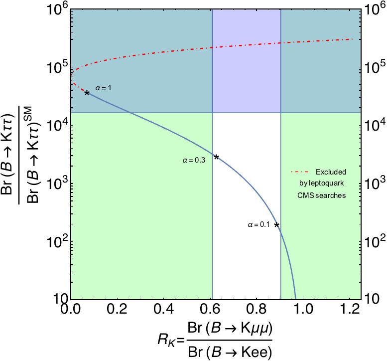
Finally, in fig. 2 we graphically display the correlation between $R_{K}$ and $B\to K\tau\tau$ for $f=1$ , that is, the case in which we keep the leading term only in the expansion in the leptonic Yukawas. In this case there is only one NP parameter controlling both processes, a variation of which produces the curve shown. Allowed experimental values at $90\%$ CL correspond to the white region, and one can see that accommodating $R_{K}$ leads to a $\mathcal{B}(B\to K\tau\tau)$ that is a few $\times 10^{3}$ larger than the SM value. If the effect is produced by a leptoquark, then CMS bounds rule out part of the line, see the Sec.VI for details.

VI A Leptoquark Model

The leptoquark particles that couple to SM fermions via operators of dimension $d\leq 4$ are either spin-0 or spin-1 bosons and they can be sorted out in terms of their quantum numbers (see [35, 36, 37, 38] and the appendix for details). There is a total of 5 scalars and 5 vector bosons as shown in tabs. 5 and 5. Assuming that their masses are above the electro-weak scale, we compute their contribution to the 4-fermion operators of the SMEFT in tab. 2. In this table one can see that only 5 of the scalar and 3 of the vector boson leptoquarks contribute to $B$ -physics and the coefficients they produce for the operators in the low-energy Lagrangian of eqs. (2,3,5) are given in Tab 2.

The number of independent operators that enter neutral-current $B$ (semi-)leptonic decays is, after imposing the full $SU(2)_{L}\times U(1)_{Y}$ symmetry, 6, whereas there are 4 charged current operators in eq. (5) which receive contributions from leptoquark models. There is therefore a priori enough potential experimental inputs to non-trivially test the hypothesis of a leptoquark in $B$ -physics.

The crucial test for these models however would be the detection of the leptoquark resonances. Since they carry color, the LHC is a powerful tool in the search for leptoquarks, which has however yielded only bounds so far, pushing the mass scale to the TeV range [90, 91].

Using Table 2 and the previous EFT study of the experimental data, it is straight-forward to select the leptoquark model that would better fit the data: a hyper-charge $2/3$ , $SU(2)_{L}$ -singlet, color-fundamental vector boson. The Lagrangian reads:

\displaystyle\mathcal{L}_{V}

\displaystyle=

\displaystyle(V_{-2/3}^{\mu})^{\dagger}\left(D^{2}+M^{2}\right)(V_{-2/3})_{\mu}+\left(g_{\ell q}\,\bar{\ell}_{L}\gamma_{\mu}q_{L}+g_{ed}\,\bar{e}_{R}\gamma_{\mu}d_{R}\right)\,V^{\mu}_{-2/3}+{\rm h.c.},

(58)

where gauge and flavor indices have been omitted. Note that this model avoids the contributions to $C_{\nu}$ since the $SU(2)_{L}$ contraction only couples up quarks to neutrinos and down quarks to electrons $\bar{q}_{L}\ell_{L}=\bar{u}_{L}\nu_{L}+\bar{d}_{L}e_{L}$ , hence $C_{q}^{(1)}=C_{q}^{(3)}$ . Also note that this model generates the chiral structure for the semi-leptonic operators suggested by data.

The flavor structure is the decisive part of the model and the focus of this work. We will use the MFV hypothesis, which was studied in the context of leptoquarks in Ref. [92]. Here we will implement our hypothesis in two ways:

•

Minimal Lepton Flavor Violation

If we formally impose only the flavor symmetry of the leptons, $SU(3)_{\ell}\times SU(3)_{e}\times U(1)_{L}\times U(1)_{e-\ell}$ , we have that $g_{q\ell}V_{-2/3}$ should transform as a $(3,1)_{1,-1}$ and $g_{ed}V_{-2/3}$ as $(1,3)_{1,1}$ . MLFV prescribes that $g_{q\ell,ed}$ should be built out of Yukawas, in this case $Y_{e}=\varepsilon_{e}\hat{Y}_{e}$ . Triality, which is the conservation of fundamental indices modulo 3 [93], prevents building a $(3,1)$ or $(1,3)$ representation from any number of Yukawas $(3,\bar{3})$ . ⁴⁴ 4 A combination of $n$ $Y_{e}$ ’s (with triality $(1,2)$ ) and $m$ $Y_{e}^{\dagger}$ ’s (with triality $(2,1)$ ) has triality ( $n+2m$ mod $3$ , $m+2n$ mod $3$ ). Although it looks like the two final trialities are unrelated, the sum of the two is always $0$ mod $3$ ; this implies that only the trialities $(0,0),(1,2),(2,1)$ are possible and remember that a representation $(3,1)$ has triality $(1,0)$ . This means that we have to assign flavor to $V_{-2/3}$ , the simplest choice being a fundamental of either $SU(3)$ flavor group. Of the possible choices, the one that yields unsuppressed LUV in the $Q_{\ell q}$ operators is:

\displaystyle V^{\mu}_{-2/3}

\displaystyle\sim(3,1)_{1,-1}\,,

\displaystyle g_{\ell q}

\displaystyle=g_{q}\hat{Y}_{e}\,,

\displaystyle g_{de}

\displaystyle=g_{d}\varepsilon_{e}^{*}\,,

(59)

where $g_{q,d}$ have a quark flavor index but no lepton index and we neglect higher powers in Yukawas. There is an interesting alternative to this scenario that however leads to the same low energy Lagrangian. Indeed, one might object that the above model inserts Yukawa couplings as prescribed by MFV but does not justify how those Yukawas got there in the first place, and is in this sense incomplete. A solution to this is the gauge flavor symmetry scenario [94]. In this case the Yukawas are the vev of the inverse of some scalar fields, $\mathcal{Y}_{e}$ that do transform ( $\mathcal{Y}_{e}\sim(\bar{3}\,,3)$ ) under the gauged flavor group: $Y_{e}\propto 1/\left\langle\mathcal{Y}_{e}\right\rangle$ . The Lagrangian would be, choosing $V_{-2/3}\sim(3,1)$ :

\displaystyle\mathcal{L}_{V}

\displaystyle=

\displaystyle(V_{-2/3}^{\mu})^{\dagger}\left(D^{2}+M^{2}+\lambda_{e}\,\mathcal{Y}_{e}^{\dagger}\mathcal{Y}_{e}\right)(V_{-2/3})_{\mu}+g_{q}\bar{\ell}_{L}\gamma_{\mu}q_{L}\,V^{\mu}_{-2/3}+{\rm h.c.},

(60)

Note that the coupling to $\bar{e}_{R}\gamma_{\mu}d_{R}$ requires an irrelevant operator. If $M^{2}$ is negligible with respect to $\mathcal{Y}_{e}$ , a case in which all operators would be marginal and the theory classically conformal, the effective operator $Q_{\ell q}^{(1)}$ has a coefficient $g_{q}g_{q}^{*}/\left\langle\mathcal{Y}_{e}^{\dagger}\mathcal{Y}_{e}\right\rangle\propto Y_{e}Y_{e}^{\dagger}$ , just as in eq. (16). Such a model however faces the more pressing question of renormalizability, due to the presence of massive vector bosons. In this sense one can postulate a strong sector in the spirit of QCD that yields as a composite state the vector boson $V_{-2/3}^{\mu}$ as a “ $\rho$ ” particle, whereas the flavor structure is dictated by the short distance physics of a gauged flavor symmetry model. Also note that a scalar leptoquark would yield a renormalizable theory.

In both cases, at low energy the coefficients of the operators are, neglecting the coupling $g_{d}\varepsilon_{e}$ :

\frac{\alpha_{e}}{\pi}\lambda_{ts}\delta C_{9}=-\frac{v^{2}}{M^{2}}\left(\frac{m_{\mu}}{m_{\tau}}\right)^{2}({g}_{q}^{s})^{*}{g}_{q}^{b}

(61)

where $g_{i}$ is $i$ -th component of the quark-family vector $g_{\ell q}$ , we have already made the rotation to the down-type quark mass basis and $\delta C_{10}=-\delta C_{9}$ . The modification to the charged current Lagrangian is:

\displaystyle\epsilon_{L}^{kj,\tau}=\frac{1}{2}\frac{v^{2}}{M^{2}}\sum_{k}\frac{V_{ik}}{V_{ij}}({g}_{q}^{k})^{*}{g}^{j}_{q}\,.

(62)

In fig. 3 we show the experimental constraints on the plane of the (real) leptoquark couplings $g_{q}^{s}$ and $g_{q}^{b}$ and using $M=0.75$ TeV. The gray band corresponds to the perturbativity bound $g_{q}^{i}=\sqrt{4\pi}$ . Finally, this model has to confront direct searches at the LHC. Searches for vector leptoquarks decaying to a $b$ quark and a $\tau$ lepton have been done by CMS, setting a limit on the mass $M>600$ GeV [90, 91].⁵⁵ 5 In deriving this bound we have used branching ratios to $b\tau$ and $t\nu_{\tau}$ of $50\%$ .

•

Quark and Lepton Minimal Flavor Violation.

If we now consider the whole flavor group for both quarks and leptons, the number of free parameters decreases since the quark flavor structure is now dictated by the up type Yukawas. Like in the previous case, triality implies that $V^{\mu}_{2/3}$ has to transform under the flavor group. We will write the quark flavor group as $U(3)^{3}=SU(3)_{q}\times SU(3)_{u}\times SU(3)_{d}\times U(1)_{B}\times U(1)_{u-q}\times U(1)_{d-q}$ . The choice of flavor transformations that yields the operator $Q_{\ell q}$ with QFV and LUV is:

\displaystyle V_{-2/3}

\displaystyle\sim(1,3)_{1,-1}\times(1,3,1)_{1/3,1,1}\,,

\displaystyle g_{q\ell}

\displaystyle=g\hat{Y}_{u}^{\dagger}\otimes\hat{Y}_{e}\,,

\displaystyle g_{de}

\displaystyle=g^{\prime}\varepsilon_{e}^{*}\varepsilon_{d}\hat{Y}_{u}\otimes\hat{Y}_{d}^{\dagger}\,,

(63)

where now $g,g^{\prime}$ are overall flavorless constants and note that the $U(1)$ charge assignment is consistent with hypercharge. This dictates that the coefficients of the operators are, neglecting $g^{\prime}\varepsilon_{e}^{*}\varepsilon_{d}$ :

\frac{\alpha_{e}}{\pi}\delta C_{9}=-\frac{v^{2}}{M^{2}}\left(\frac{m_{\mu}}{m_{\tau}}\right)^{2}\left|g\right|^{2}.

(64)

and $\delta C_{10}=-\delta C_{9}$ . Note that the sign of the contribution is fixed and $g\sim 1$ implies $M\sim 600$ GeV, which is around the current experimental CMS limit. The MLFV prediction in fig. 2 depends on the combination $g/M$ for this model. The points marked as $\alpha=g^{2}/(4\pi)=0.1,0.3,1$ correspond to a mass $M=600$ GeV. The red dashed part of the line has $\alpha\geq 1$ and we consider it excluded.

VII Conclusions

We have analyzed various anomalies in the neutral- and charged-current (semi)leptonic $B$ -meson decays that suggest the presence of new interactions violating lepton universality. Although this leads to the expectation of sizable lepton flavor violation in $B$ decays (as discussed recently and abundantly in the literature), we have shown that this is not the case in a general class of new-physics scenarios with minimal flavor violation. Namely, in case one can neglect flavor effects from the neutrino mass generation mechanism, one finds that charged-lepton flavor is preserved but universality is not, with the violation of the latter being controlled by charged-lepton masses. In these scenarios, the skewed ratio $R_{K}$ found experimentally is explained by new physics coupled more strongly to muons than to electrons. Furthermore, the tauonic $B$ -decays receive a strong enhancement due to the relative factor $(m_{\tau}/m_{\mu})^{2}$ in the corresponding couplings to the leptons.

We have first explored the phenomenological consequences of this hypothesis at the level of the effective operators of the standard model effective field theory and have selected a linear combination of them involving only $SU(2)_{L}$ doublets as the most plausible explanation for all the anomalies. Accommodating $R_{K}$ in this scenario implies an $\mathcal{O}(10^{3})$ boost, with respect to the standard model, of the $B_{s}\to\tau\tau$ , $B\to K^{(*)}\tau\tau$ and $B\to K\nu\bar{\nu}$ decay rates. The predicted rates to charged $\tau$ leptons are an order of magnitude below the current experimental limits and they could be tested in future experiments at $B$ factories. The decay into neutrinos, which is much better measured, poses a strong constraint on the new physics that can be accounted for naturally if it does not couple neutrinos and down-type quarks. As for charged current decays, the enhancement for tauonic decays is approximately the same enhancement that the standard model presents due to charged current decays occurring at tree level as opposed to 1-loop rare decays. In fact, a remarkable outcome is that $R_{K}$ , $R_{D^{(*)}}$ and $B^{-}\to\tau^{-}\bar{\nu}$ anomalies can be explained simultaneously and naturally with new-physics effective mass in the multi-TeV range. A manifest advantage of using an effective field theory setup is that it shows a model-independent interplay between the $B$ -decays of interest and top-physics, with the $t\to q\nu\tau$ turning to be a complementary and powerful way to test these scenarios.

Finally, as an illustration of our hypothesis in model building, we have surveyed the contributions of all possible spin-0 and spin-1 leptoquark particle models to $B$ -decays. We have first projected their contributions into the effective operators of the standard model effective field theory, integrating the leptoquark fields out, and then we have applied the conclusions of our study to select a unique model that is better suited to fit the data (even if there is room for other possibilities): an $SU(2)_{L}$ singlet, color-fundamental vector boson of hypercharge $2/3$ . It was shown how the assumed flavor structure of minimal lepton flavor violation could arise from a Lagrangian with operators of dimension $\leq 4$ , and a particular case was presented in which the flavor structure arose from the vev of scalar fields.

VIII Acknowledgments

This work was supported in part by DOE grants DE-SC000991 and DE-SC0009919. JMC has received funding from the People Programme (Marie Curie Actions) of the European Union’s Seventh Framework Programme (FP7/2007-2013) under REA grant agreement n PIOF-GA-2012-330458 and acknowledges the Spanish Ministerio de Economía y Competitividad and european FEDER funds under the contract FIS2011-28853-C02-01 for support.

Appendix A Leptoquark Bosons

LQ	$C_{\ell q}^{(1)}$	$C_{\ell q}^{(3)}$	$C_{\ell d}$	$C_{qe}$	$C_{ed}$	$C_{\ell edq}$	$C_{lequ}^{(1)}$	$C_{lequ}^{(3)}$	$C_{eu}$	$C_{\ell u}$
$\Delta_{1/3}$	$\frac{y_{\ell q}^{\beta i,A}(y_{\ell q}^{\alpha j,A})^{*}}{4M^{2}}$	$-\frac{y_{\ell q}^{\beta i,A}(y_{\ell q}^{\alpha j,A})^{*}}{4M^{2}}$	0	0	0	0	$-\frac{y_{eu}^{\beta i,A}(y_{\ell q}^{\alpha j,A})^{*}}{2M^{2}}$	$\frac{y_{eu}^{\beta i,A}(y_{\ell q}^{\alpha j,A})^{*}}{8M^{2}}$	$\frac{y_{eu}^{\beta i,A}(y_{eu}^{\alpha j,A})^{*}}{2M^{2}}$	0
$\vec{\Delta}_{1/3}$	$\frac{3y_{\ell q}^{\prime\beta i,A}(y_{\ell q}^{\prime\alpha j,A})^{*}}{4M^{2}}$	$\frac{y_{\ell q}^{\prime\beta i,A}(y_{\ell q}^{\prime\alpha j,A})^{*}}{4M^{2}}$	0	0	0	0	0	0	0	0
$\Delta_{7/6}$	0	0	0	$-\frac{y_{eq}^{\alpha i,A}(y_{eq}^{\beta j,A})^{*}}{2M^{2}}$	0	0	$-\frac{y_{\ell u}^{\alpha i,A}(y_{eq}^{\beta j,A})^{*}}{2M^{2}}$	$-\frac{y_{\ell u}^{\alpha i,A}(y_{eq}^{\beta j,A})^{*}}{8M^{2}}$	0	$-\frac{y_{\ell u}^{\alpha i,A}(y_{\ell u}^{\beta j,A})^{*}}{2M^{2}}$
$\Delta_{1/6}$	0	0	$-\frac{y_{\ell d}^{\alpha i\,A}(y_{\ell d}^{\beta j,A})^{*}}{2M^{2}}$	0	0	0	0	0	0	0
$\Delta_{4/3}$	0	0	0	0	$\frac{y_{ed}^{\beta i\,A}(y_{ed}^{\alpha j,A})^{*}}{2M^{2}}$	0	0	0	0	0
$V^{\mu}_{2/3}$	$-\frac{g_{\ell q}^{\alpha i,A}(g_{\ell q}^{\beta j,A})^{*}}{2M^{2}}$	$-\frac{g_{\ell q}^{\alpha i,A}(g_{\ell q}^{\beta j,A})^{*}}{2M^{2}}$	0	0	$-\frac{g_{ed}^{\alpha i,A}(g_{ed}^{\beta j,A})^{*}}{M^{2}}$	$\frac{2g_{\ell q}^{\alpha i,A}(g_{ed}^{\beta j,A})^{*}}{M^{2}}$	0	0	0	0
$\vec{V}^{\mu}_{2/3}$	$-\frac{3g_{\ell q}^{\prime\alpha i,A}(g_{\ell q}^{\prime\beta j,A})^{*}}{2M^{2}}$	$\frac{g_{\ell q}^{\prime\alpha i,A}(g_{\ell q}^{\prime\beta j,A})^{*}}{2M^{2}}$	0	0	0	0	0	0	0	0
$V^{\mu}_{5/6}$	0	0	$\frac{g_{\ell d}^{\alpha j,A}(g_{\ell d}^{\beta i,A})^{*}}{M^{2}}$	$\frac{g_{eq}^{\alpha j,A}(g_{eq}^{\beta i,A})^{*}}{M^{2}}$	$\frac{2g_{\ell d}^{\alpha j,A}(g_{eq}^{\beta i,A})^{*}}{M^{2}}$	0	0	0	0	0
$V^{\mu}_{5/3}$	0	0	0	0	0	0	0	0	$-\frac{g_{eu}^{\alpha i\,A}(g_{eu}^{\beta j,A})^{*}}{M^{2}}$	0
$V^{\mu}_{1/6}$	0	0	0	0	0	0	0	0	0	$\frac{g_{\ell u}^{\alpha j\,A}(g_{\ell u}^{\beta i})^{*}}{M^{2}}$

Table 1: Tree-level leptoquark contributions to the sixth-dimensional four-fermion operators of the SMEFT with flavor indexes

(Q_{\ell q}^{(1)})^{\alpha\beta,ij}=(\overline{q}^{j}\gamma^{\mu}q_{L}^{i})(\bar{\ell}^{\alpha}\gamma_{\mu}\ell^{\beta})

and so forth. The internal leptoquark index,

A

, is summed over.

LQ	$C_{9}$	$C_{10}$	$C_{9}^{\prime}$	$C_{10}^{\prime}$	$C_{S}$	$C_{S}^{\prime}$	$C_{\nu}$	$C_{\nu}^{\prime}$
$\Delta_{1/3}$	0	0	0	0	0	0	$\frac{1}{2}y_{\ell q}^{\beta b,A}(y_{\ell q}^{\alpha j,A})^{*}$	0
$\vec{\Delta}^{\prime}_{1/3}$	$y_{\ell q}^{\prime\beta b,A}(y_{\ell q}^{\prime\alpha j,A})^{*}$	$-y_{\ell q}^{\prime\beta b,A}(y_{\ell q}^{\prime\alpha j,A})^{*}$	0	0	0	0	$\frac{1}{2}y_{\ell q}^{\prime\beta b,A}(y_{\ell q}^{\prime\alpha j,A})^{*}$	0
$\Delta_{7/6}$	$-\frac{1}{2}y_{eq}^{\alpha b,A}(y_{eq}^{\beta j,A})^{*}$	$-\frac{1}{2}y_{eq}^{\alpha b,A}(y_{eq}^{\beta j,A})^{*}$	0	0	0	0	0	0
$\Delta_{1/6}$	0	0	$-\frac{1}{2}y_{\ell d}^{\alpha b,A}(y_{\ell d}^{\beta j,A})^{*}$	$\frac{1}{2}y_{\ell d}^{\alpha b,A}(y_{\ell d}^{\beta j,A})^{*}$	0	0	0	$-\frac{1}{2}y_{\ell d}^{\alpha b,A}(y_{\ell d}^{\beta j,A})^{*}$
$\Delta_{4/3}$	0	0	$\frac{1}{2}y_{ed}^{\beta b,A}(y_{ed}^{\alpha j,A})^{*}$	$\frac{1}{2}y_{ed}^{\beta b,A}(y_{ed}^{\alpha j,A})^{*}$	0	0	0	0
$V^{\mu}_{2/3}$	$-g_{\ell q}^{\alpha b,A}(g_{\ell q}^{\beta j,A})^{*}$	$g_{\ell q}^{\alpha b,A}(g_{\ell q}^{\beta j,A})^{*}$	$-g_{ed}^{\alpha b,A}(g_{ed}^{\beta j,A})^{*}$	$-g_{ed}^{\alpha b,A}(g_{ed}^{\beta j,A})^{*}$	$2g_{\ell q}^{\alpha b,A}(g_{ed}^{\beta j,A})^{*}$	$2(g_{\ell q}^{\beta j,A})^{*}g_{ed}^{\alpha b,A}$	0	0
$\vec{V}^{\mu}_{2/3}$	$-g_{\ell q}^{\prime\alpha b,A}(g_{\ell q}^{\prime\beta j,A})^{*}$	$g_{\ell q}^{\prime\alpha b,A}(g_{\prime\ell q}^{\beta j,A})^{*}$	0	0	0	0	$-2\,g_{\ell q}^{\prime\alpha b,A}(g_{\ell q}^{\prime\beta j,A})^{*}$	0
$V^{\mu}_{5/6}$	$g_{eq}^{\alpha j,A}(g_{eq}^{\beta b,A})^{*}$	$g_{eq}^{\alpha j,A}(g_{eq}^{\beta b,A})^{*}$	$g_{\ell d}^{\alpha j,A}(g_{\ell d}^{\beta b,A})^{*}$	$-g_{\ell d}^{\alpha j,A}(g_{\ell d}^{\beta b,A})^{*}$	$2g_{\ell d}^{\alpha j,A}(g_{eq}^{\beta b,A})^{*}$	$2(g_{\ell d}^{\beta b,A})^{*}g_{eq}^{\alpha j,A}$	0	$g_{\ell d}^{\alpha j,A}(g_{\ell d}^{\beta b,A})^{*}$

Table 2: Contributions of the different leptoquarks to the

b\to d_{j}\ell_{\alpha}\ell_{\beta}

operators with

j=d,s

and

\alpha,\beta=e,\mu,\tau.

The normalization

4\pi^{2}/(e^{2}\lambda_{ts})\,v^{2}/M^{2}

has been factored out and

A

is an internal leptoquark index summed over.

For the new leptoquark boson to couple to SM particles through dimension $\leq 4$ operators its spin must be 0 or 1, and the interactions with SM fields described by:

$\displaystyle\mathcal{L}_{\Delta}$	$\displaystyle=$	$\displaystyle\left(y_{\ell u}\,\bar{\ell}_{L}\,u_{R}+y_{eq}\,\bar{e}_{R}\,i\tau_{2}\,q_{L}\right)\,\Delta_{-7/6}+y_{\ell d}\,\bar{\ell}_{L}\,d_{R}\,\Delta_{-1/6}+\left(y_{\ell q}\,\bar{\ell}^{c}_{L}i\tau_{2}\,q_{L}+y_{eu}\bar{e}_{R}^{c}\,u_{R}\right)\,\Delta_{1/3}$	(65)
	$\displaystyle+$	$\displaystyle y_{ed}\bar{e}^{c}_{R}\,d_{R}\,\Delta_{4/3}+y_{\ell q}^{\prime}\,\bar{\ell}^{c}_{L}i\tau_{2}\vec{\tau}q_{L}\,\cdot\vec{\Delta}^{\prime}_{1/3}+{\rm h.c.},$	(65)
$\displaystyle\mathcal{L}_{V}$	$\displaystyle=$	$\displaystyle\left(g_{\ell q}\,\bar{\ell}_{L}\gamma_{\mu}q_{L}+g_{ed}\,\bar{e}_{R}\gamma_{\mu}d_{R}\right)\,V^{\mu}_{-2/3}+g_{eu}\,\bar{e}_{R}\gamma_{\mu}u_{R}\,V^{\mu}_{5/3}+g_{\ell q}^{\prime}\,\bar{\ell}_{L}\gamma_{\mu}\vec{\tau}q_{L}\,\cdot\vec{V}^{\prime\mu}_{-2/3}$	(66)
	$\displaystyle+$	$\displaystyle\left(g_{\ell d}\,\bar{\ell}_{L}\gamma_{\mu}d_{R}^{c}+g_{eq}\,\bar{e}_{R}\gamma_{\mu}q^{c}_{L}\right)\,V_{-5/6}^{\mu}+g_{\ell u}\,\bar{\ell}_{L}\gamma_{\mu}u_{R}^{c}\,V^{\mu}_{1/6}+{\rm h.c.},$	(66)

where $SU(2)_{L}$ and flavor indices have been omitted, each leptoquark is labeled by its hypercharge and $\Delta$ and $V$ denote scalars and vector boson respectively. The SM charge assignments corresponding to each case are displayed in tabs. (5) and (5).

Bilinear $(J)$	$SU(3)_{c}$	$SU(2)_{L}$	$U(1)_{Y}$
$\overline{\ell}_{L}^{c}q_{L}$	$\bar{3}$	1 ,3	1/3
$\overline{e}_{R}^{c}u_{R}$	$\bar{3}$	1	1/3
$\bar{\ell}_{L}u_{R}$	$\bar{3}$	2	-7/6
$\overline{e}_{R}q_{L}$	$\bar{3}$	2	-7/6
$\bar{\ell}_{L}d_{R}$	$\bar{3}$	2	-1/6
$\overline{e}_{R}^{c}d_{R}$	$\bar{3}$	1	4/3

Figure 4: Charge assignment for leptoquark scalars,

\Delta

, as a function of the SM fermion current to which they couple.

Bilinear $(J^{\mu})$	$SU(3)_{c}$	$SU(2)_{L}$	$U(1)_{Y}$
$\overline{\ell}_{L}\gamma_{\mu}q_{L}$	$\bar{3}$	1 ,3	-2/3
$\overline{e}_{R}\gamma_{\mu}d_{R}$	$\bar{3}$	1	-2/3
$\bar{\ell}_{L}^{c}\gamma_{\mu}d_{R}$	$\bar{3}$	2	5/6
$\overline{e}_{R}^{c}\gamma_{\mu}q_{L}$	$\bar{3}$	2	5/6
$\overline{e}_{R}\gamma_{\mu}u_{R}$	$\bar{3}$	1	-5/3
$\bar{\ell}_{L}^{c}\gamma_{\mu}u_{R}$	$\bar{3}$	2	-1/6

Figure 5: Charge assignment for leptoquark vector-bosons,

V_{\mu}

, as a function of the SM fermion current to which they couple.

All the bosons should be fundamentals of the color group and therefore its mass high enough not to have been produced and detected at the LHC. As for the hyper-charges we note that the “coincidences” in tabs. (5) and (5) are not so but follow from the fact that Yukawa terms in the SM can be build for quarks and leptons with the same hyper-charge $1/2$ scalar.

We shall write the Lagrangian for the bosons, respectively, as:

	$\displaystyle\mathcal{L}_{\Delta}$	$\displaystyle=-\Delta^{\dagger}\left(\left[D^{2}+M_{\Delta}^{2}\right]\Delta-y^{\dagger}J\right)+J^{\dagger}y\,\Delta$		(67)
	$\displaystyle\mathcal{L}_{V}$	$\displaystyle=\left(V^{\mu}\right)^{\dagger}\left(\left[D^{2}+M_{V}^{2}\right]V_{\mu}+g^{\dagger}J_{\mu}\right)+\left(J^{\mu}\right)^{\dagger}\,g\,V_{\mu}$		(68)

where $J$ and $J_{\mu}$ are the bilinears in tabs. (5) and (5), $D^{2}=D^{\mu}D_{\mu}$ is the covariant derivative containing the SM gauge bosons, $M^{2}>0$ and flavor indices have been omitted for clarity. The way the Lagrangian is written is useful for the integration of the heavy bosons; the term in parenthesis equated to zero is the E.O.M. and vanishes on-shell.

A.1 Contributions to low energy processes

Integrating out the leptoquark bosons in eq. (67) yields formally the following effective Lagrangian,

	$\displaystyle\mathcal{L}_{\rm eff}$	$\displaystyle=J^{\dagger}y\frac{1}{M_{\Delta}^{2}}y^{\dagger}J+\mathcal{O}\left(\frac{1}{M_{\Delta}^{4}}\right)$		(69)
	$\displaystyle\mathcal{L}_{\rm eff}$	$\displaystyle=-J^{\dagger}_{\mu}\,g\frac{1}{M_{V}^{2}}g^{\dagger}J^{\mu}+\mathcal{O}\left(\frac{1}{M_{V}^{4}}\right)$		(70)

which can be projected in basis of operators of the SM, as is done in tab. (2) and, after EWSB, contributes to the $B$ -meson semi-leptonic Lagrangian as specified in tab. (2).

References

[1] G. Hiller and F. Kruger, Phys.Rev. D69, 074020 (2004), eprint hep-ph/0310219.
[2] C. Bobeth, G. Hiller, and G. Piranishvili, JHEP 0712, 040 (2007), eprint 0709.4174.
[3] R. Aaij et al. (LHCb collaboration), Phys.Rev.Lett. 113, 151601 (2014a), eprint 1406.6482.
[4] R. Aaij et al. (LHCb collaboration), Phys.Rev.Lett. 111, 191801 (2013a), eprint 1308.1707.
[5] R. R. Horgan, Z. Liu, S. Meinel, and M. Wingate, Phys.Rev.Lett. 112, 212003 (2014a), eprint 1310.3887.
[6] R. R. Horgan, Z. Liu, S. Meinel, and M. Wingate, Phys.Rev. D89, 094501 (2014b), eprint 1310.3722.
[7] A. Khodjamirian, T. Mannel, and Y. Wang, JHEP 1302, 010 (2013), eprint 1211.0234.
[8] R. Aaij et al. (LHCb), JHEP 1307, 084 (2013b), eprint 1305.2168.
[9] R. Aaij et al. (LHCb collaboration), Phys.Rev.Lett. 111, 112003 (2013c), eprint 1307.7595.
[10] R. Aaij et al. (LHCb), JHEP 1406, 133 (2014b), eprint 1403.8044.
[11] L. Randall and M. B. Wise, Phys.Lett. B303, 135 (1993), eprint hep-ph/9212315.
[12] C. G. Boyd and B. Grinstein, Nucl.Phys. B451, 177 (1995), eprint hep-ph/9502311.
[13] A. Matyja et al. (Belle Collaboration), Phys.Rev.Lett. 99, 191807 (2007), eprint 0706.4429.
[14] A. Bozek et al. (Belle Collaboration), Phys.Rev. D82, 072005 (2010), eprint 1005.2302.
[15] J. Lees et al. (The BaBar Collaboration), Phys.Rev. D88, 072012 (2013a), eprint 1303.0571.
[16] S. Fajfer, J. F. Kamenik, and I. Nisandzic, Phys.Rev. D85, 094025 (2012), eprint 1203.2654.
[17] D. Becirevic, N. Kosnik, and A. Tayduganov, Phys.Lett. B716, 208 (2012), eprint 1206.4977.
[18] K. Olive et al. (Particle Data Group), Chin.Phys. C38, 090001 (2014).
[19] A. Celis, M. Jung, X.-Q. Li, and A. Pich, JHEP 1301, 054 (2013), eprint 1210.8443.
[20] S. Descotes-Genon, J. Matias, and J. Virto, Phys.Rev. D88, 074002 (2013a), eprint 1307.5683.
[21] F. Beaujean, C. Bobeth, and D. van Dyk, Eur.Phys.J. C74, 2897 (2014), eprint 1310.2478.
[22] J. Lyon and R. Zwicky (2014), eprint 1406.0566.
[23] R. Alonso, B. Grinstein, and J. Martin Camalich, Phys.Rev.Lett. 113, 241802 (2014a), eprint 1407.7044.
[24] G. Hiller and M. Schmaltz, Phys.Rev. D90, 054014 (2014), eprint 1408.1627.
[25] D. Ghosh, M. Nardecchia, and S. Renner, JHEP 1412, 131 (2014), eprint 1408.4097.
[26] T. Hurth, F. Mahmoudi, and S. Neshatpour, JHEP 1412, 053 (2014), eprint 1410.4545.
[27] W. Altmannshofer and D. M. Straub (2014), eprint 1411.3161.
[28] S. L. Glashow, D. Guadagnoli, and K. Lane (2014), eprint 1411.0565.
[29] S. Jäger and J. Martin Camalich (2014), eprint 1412.3183.
[30] B. Bhattacharya, A. Datta, D. London, and S. Shivashankara, Phys.Lett. B742, 370 (2015), eprint 1412.7164.
[31] A. Crivellin, G. D’Ambrosio, and J. Heeck (2015a), eprint 1501.00993.
[32] S. D. Aristizabal, F. Staub, and A. Vicente (2015), eprint 1503.06077.
[33] S. M. Boucenna, J. W. F. Valle, and A. Vicente (2015), eprint 1503.07099.
[34] A. Crivellin, L. Hofer, J. Matias, U. Nierste, S. Pokorski, et al. (2015b), eprint 1504.07928.
[35] W. Buchmuller, R. Ruckl, and D. Wyler, Phys.Lett. B191, 442 (1987).
[36] S. Davidson, D. C. Bailey, and B. A. Campbell, Z.Phys. C61, 613 (1994), eprint hep-ph/9309310.
[37] J. L. Hewett and T. G. Rizzo, Phys.Rev. D56, 5709 (1997), eprint hep-ph/9703337.
[38] Y. Sakaki, M. Tanaka, A. Tayduganov, and R. Watanabe, Phys.Rev. D88, 094012 (2013), eprint 1309.0301.
[39] B. Gripaios, M. Nardecchia, and S. Renner (2014), eprint 1412.1791.
[40] S. Sahoo and R. Mohanta (2015), eprint 1501.05193.
[41] I. de Medeiros Varzielas and G. Hiller (2015), eprint 1503.01084.
[42] D. Bečirević, S. Fajfer, and N. Košnik (2015), eprint 1503.09024.
[43] S. Glashow, J. Iliopoulos, and L. Maiani, Phys.Rev. D2, 1285 (1970).
[44] B. Grinstein, M. J. Savage, and M. B. Wise, Nucl.Phys. B319, 271 (1989).
[45] G. Buchalla, A. J. Buras, and M. E. Lautenbacher, Rev.Mod.Phys. 68, 1125 (1996), eprint hep-ph/9512380.
[46] K. G. Chetyrkin, M. Misiak, and M. Munz, Phys.Lett. B400, 206 (1997), eprint hep-ph/9612313.
[47] V. Cirigliano, J. Jenkins, and M. Gonzalez-Alonso, Nucl.Phys. B830, 95 (2010), eprint 0908.1754.
[48] V. Cirigliano, M. Gonzalez-Alonso, and M. L. Graesser, JHEP 1302, 046 (2013), eprint 1210.4553.
[49] S. Weinberg, Phys.Rev.Lett. 43, 1566 (1979).
[50] W. Buchmuller and D. Wyler, Nucl.Phys. B268, 621 (1986).
[51] B. Grzadkowski, M. Iskrzynski, M. Misiak, and J. Rosiek, JHEP 1010, 085 (2010), eprint 1008.4884.
[52] G. Buchalla and O. Cata, JHEP 1207, 101 (2012), eprint 1203.6510.
[53] A. J. Buras, J. Girrbach-Noe, C. Niehoff, and D. M. Straub (2014), eprint 1409.4557.
[54] S. Antusch, C. Biggio, E. Fernandez-Martinez, M. Gavela, and J. Lopez-Pavon, JHEP 0610, 084 (2006), eprint hep-ph/0607020.
[55] A. Filipuzzi, J. Portoles, and M. Gonzalez-Alonso, Phys.Rev. D85, 116010 (2012), eprint 1203.2092.
[56] E. E. Jenkins, A. V. Manohar, and M. Trott, JHEP 1310, 087 (2013), eprint 1308.2627.
[57] E. E. Jenkins, A. V. Manohar, and M. Trott, JHEP 1401, 035 (2014), eprint 1310.4838.
[58] R. Alonso, E. E. Jenkins, A. V. Manohar, and M. Trott, JHEP 1404, 159 (2014b), eprint 1312.2014.
[59] R. Alonso, H.-M. Chang, E. E. Jenkins, A. V. Manohar, and B. Shotwell, Phys.Lett. B734, 302 (2014c), eprint 1405.0486.
[60] R. Alonso, G. Isidori, L. Merlo, L. A. Munoz, and E. Nardi, JHEP 1106, 037 (2011), eprint 1103.5461.
[61] M. Gavela, T. Hambye, D. Hernandez, and P. Hernandez, JHEP 0909, 038 (2009), eprint 0906.1461.
[62] R. S. Chivukula and H. Georgi, Phys.Lett. B188, 99 (1987).
[63] G. D’Ambrosio, G. Giudice, G. Isidori, and A. Strumia, Nucl.Phys. B645, 155 (2002), eprint hep-ph/0207036.
[64] V. Cirigliano, B. Grinstein, G. Isidori, and M. B. Wise, Nucl.Phys. B728, 121 (2005), eprint hep-ph/0507001.
[65] S. Davidson and F. Palorini, Phys.Lett. B642, 72 (2006), eprint hep-ph/0607329.
[66] M. Beneke, T. Feldmann, and D. Seidel, Nucl.Phys. B612, 25 (2001), eprint hep-ph/0106067.
[67] W. Altmannshofer, P. Ball, A. Bharucha, A. J. Buras, D. M. Straub, et al., JHEP 0901, 019 (2009), eprint 0811.1214.
[68] C. Bobeth, G. Hiller, and D. van Dyk, JHEP 1007, 098 (2010), eprint 1006.5013.
[69] U. Egede, T. Hurth, J. Matias, M. Ramon, and W. Reece, JHEP 1010, 056 (2010), eprint 1005.0571.
[70] S. Descotes-Genon, J. Matias, M. Ramon, and J. Virto, JHEP 1301, 048 (2013b), eprint 1207.2753.
[71] S. Jäger and J. Martin Camalich, JHEP 1305, 043 (2013), eprint 1212.2263.
[72] W. Altmannshofer and D. M. Straub, Eur.Phys.J. C73, 2646 (2013), eprint 1308.1501.
[73] T. Hurth and F. Mahmoudi, JHEP 1404, 097 (2014), eprint 1312.5267.
[74] T. L. Collaboration (LHCb) (2015).
[75] W. Altmannshofer and D. M. Straub (2015), eprint 1503.06199.
[76] S. Descotes-Genon, L. Hofer, J. Matias, and J. Virto, JHEP 1412, 125 (2014), eprint 1407.8526.
[77] A. Bharucha, D. M. Straub, and R. Zwicky (2015), eprint 1503.05534.
[78] V. Khachatryan et al. (CMS Collaboration, LHCb Collaboration) (2014a), eprint 1411.4413.
[79] C. Bobeth, M. Gorbahn, T. Hermann, M. Misiak, E. Stamou, et al., Phys.Rev.Lett. 112, 101801 (2014), eprint 1311.0903.
[80] K. De Bruyn, R. Fleischer, R. Knegjens, P. Koppenburg, M. Merk, et al., Phys.Rev.Lett. 109, 041801 (2012), eprint 1204.1737.
[81] C. Bobeth and U. Haisch, Acta Phys.Polon. B44, 127 (2013), eprint 1109.1826.
[82] C. Bouchard, G. P. Lepage, C. Monahan, H. Na, and J. Shigemitsu (HPQCD), Phys.Rev.Lett. 111, 162002 (2013), eprint 1306.0434.
[83] K. Flood (BaBar Collaboration), PoS ICHEP2010, 234 (2010).
[84] J. Lees et al. (BaBar Collaboration), Phys.Rev. D87, 112005 (2013b), eprint 1303.7465.
[85] O. Lutz et al. (Belle Collaboration), Phys.Rev. D87, 111103 (2013), eprint 1303.3719.
[86] S. Aoki, Y. Aoki, C. Bernard, T. Blum, G. Colangelo, et al., Eur.Phys.J. C74, 2890 (2014), eprint 1310.8555.
[87] Y. Amhis et al. (Heavy Flavor Averaging Group (HFAG)) (2014), eprint 1412.7515.
[88] A. Abulencia et al. (CDF Collaboration), Phys.Lett. B639, 172 (2006), eprint hep-ex/0510063.
[89] A. L. Kagan, G. Perez, T. Volansky, and J. Zupan, Phys.Rev. D80, 076002 (2009), eprint 0903.1794.
[90] V. Khachatryan et al. (CMS), Phys.Lett. B739, 229 (2014b), eprint 1408.0806.
[91] V. Khachatryan et al. (CMS) (2015), eprint 1503.09049.
[92] S. Davidson and S. Descotes-Genon, JHEP 1011, 073 (2010), eprint 1009.1998.
[93] H. Georgi, Front.Phys. 54, 1 (1982).
[94] B. Grinstein, M. Redi, and G. Villadoro, JHEP 1011, 067 (2010), eprint 1009.2049.

Lepton universality violation and lepton flavor conservation in BB-meson decays