Locally Repairable Regenerating Codes: Node Unavailability and the Insufficiency of Stationary Local Repair

This work follows the same distributed storage network model as introduced in the seminal work [7]. For completeness, we provide in the following detailed definitions of some key parameters. Further explanations of the system model can be found in [7].

Parameters $n$ and $k$: We denote the total number of nodes in a storage network by $n$. For any $1\leq k\leq n-1$, we say that a code can satisfy the reconstruction requirement if any $k$ nodes can be used to reconstruct the original data/file. For example, consider a network of 7 nodes. A $(7,4)$ Hamming code can be used to protect the data. We say that the Hamming code can satisfy the reconstruction requirement for $k=6$. Since any 6 nodes can construct the original file. By the same definition, the Hamming code can also satisfy the reconstruction requirement for $k=5$ and $k=4$, but cannot satisfy the reconstruction requirement for $k=3$. The smallest $k$ of the $(7,4)$ Hamming code is thus $k^{*}=4$. In general, the value of $k$ is related to the desired protection level of the system while the value of $k^{*}$ is related to actual protection level offered by the specific distributed storage code implementation.

For example, suppose the design requirement is $k=6$, we can still opt for using the $(7,4)$ Hamming code to provide the desired level of protection. However, using $(7,4)$ Hamming code may be an overkill since a $(7,4)$ Hamming code has $k^{*}=4$ and it is possible to just use a single-parity bit to achieve $k=6$.

Parameter $d$: We denote the number of nodes that a newcomer can access during repair by $d$. For example, [7] provides a detailed RC construction about how to achieve the design goal $(n,k,d)=(10,7,9)$. Namely, each newcomer can access $d=9$ helpers and any $k=7$ nodes can be used to reconstruct the original file. At the same time, [7] also provides high-level guidelines how to use the RC to achieve the design goal when $(n,k,d)=(10,7,5)$. However, the RC can be an overkill in this scenario $(n,k,d)=(10,7,5)$ since any RC construction in [7] that can achieve $(n,k,d)=(10,7,5)$ can always achieve $k^{*}=d=5$. As a result, even though the high-level design goal is to only protect against $10-7=3$ failures under the constraint of accessing only $d=5$ helpers during repair, the RC in [7] cannot take advantage of this relatively loose protection-level requirement since it always has $k^{*}\leq d=5$.

Note that the above observation does not mean that the system designer should never use the RCs [7] when the design goal is $(n,k,d)=(10,7,5)$. The reason is that these RCs with BHS have many other advantages that may be very appealing in practice, e.g., some very efficient algebraic code construction methods [19], allowing repair with $(n-d)$ simultaneous failures, and admitting efficient collaborative repair when more than one node fails [20]. The fact that $k^{*}\leq d$ for any RCs in [7] simply means that when the requirement is $(n,k,d)=(10,7,5)$, the system designer should be aware that the RCs with BHS in [7] cannot take full advantage of the relatively loose required protection level since we have in this scenario $k>d\geq k^{*}$.

In this work, we focus on the design target $k$ instead of the actual performance parameter $k^{*}$, since given the same $k$, the actual $k^{*}$ value may depend on how we implement the codes. For example, when locally repairable codes [9] are used, it is possible to design a system with $k=k^{*}>d$. However, when RCs are used together with BHS, we always have $k^{*}\leq d$ even though the target protection level may satisfy $k>d$. For any given $(n,k,d)$ values, the goal of this paper is to compare the best performance of any possible helper selection scheme that can still satisfy the desired $(n,k,d)$ values regardless whether they offer over-protection ($k>k^{*}$) or not.

Parameter $r$: We denote the maximum number of nodes that can be temporarily unavailable at any given time by $r$. Specifically, if we denote the set of unavailable nodes by $U$, then we must have $|U|\leq r$. If we also denote the failed node by $F$, the design goal is to repair node $F$ when the nodes in $U$ are unavailable. The unavailability of nodes in $U$ may be due to degenerate reads, multiple failures, or underlying network dynamics. In this work we do not consider repair collaboration. That means, even when we have multiple failures, say both nodes $i$ and $j$ fail simultaneously, we repair each node separately. For example, we set $F=i$ and $U=\{j\}$ when repairing node $i$ and we set $F=j$ and $U=\{i\}$ when repairing node $j$. Some repair cooperation schemes that jointly repair both nodes $i$ and $j$ can be found in [20].

The range of the design criteria $(n,k,d,r)$: Due to the nature of the distributed storage problem, we only consider $(n,k,d,r)$ values that satisfy

In all the results in this work, we assume implicitly that the $n$, $k$, and $d$ values satisfy (1).

Parameters $\alpha$, $\beta$, and $\mathcal{M}$: The overall file size is denoted by $\mathcal{M}$. The storage size for each node is $\alpha$, and during the repair process, the newcomer requests $\beta$ amount of traffic from each of the helpers. The total repair-bandwidth is thus $\gamma\stackrel{{\scriptstyle\Delta}}{{=}}d\beta$.

DHS: We consider the most general form of helper selection in which the helper selection at current time $\tau$ can depend on the time index $\tau$ and the history of node failures and node unavailability from all the previous time slots 1 to ($\tau-1$). We term this type of schemes the dynamic helper selection (DHS) scheme. Mathematically, for every time slot $\tau$ (or equivalently for the $\tau$-th repair) the helper set decision at time $\tau$ can be written in function form as $D_{\tau}(\{F_{i}\}_{i=1}^{\tau},\{U_{j}\}_{j=1}^{\tau})$ that returns the set of helpers the newcomer has to access at time $\tau$, where $F_{i}$ and $U_{j}$ are the failed node at time $i$ and the set of unavailable nodes at time $j$, respectively. Since the helper selection function depends on the history of the failure/unavailability patterns and can change for each different time $\tau$, we term this scheme the dynamic helper selection (DHS) scheme, for which the term “dynamic” emphasizes the time and history dependence of the helper selection rules.

SHS: A subset of the DHS schemes is the stationary helper selection (SHS) schemes that assign fixed helper sets of $d$ nodes to each combination of a failed node and a set of unavailable nodes. Mathematically, the helper set decision at time $\tau$ in SHS can be written in function form as $D(F_{\tau},U_{\tau})$. The function $D(\cdot,\cdot)$ does not change with respect to the value of $\tau$ and the input arguments of $D(\cdot,\cdot)$ are $F_{\tau}$ and $U_{\tau}$, instead of the entire history $\{F_{i}\}_{i=1}^{\tau}$ and $\{U_{j}\}_{j=1}^{\tau}$. The idea is that, for a given node failure and a given set of unavailable nodes, the same helper set is used at any time instant. We can see that this construction is stationary because the helper sets do not change with time and only depend on current time $\tau$ failure and node unavailability information.

All existing (non-blind) helper selection schemes can be interpreted as a form of SHS. For example, a popular way of helper selection when there are $r$ temporarily unavailable nodes [15, 14, 11, 17] is as follows. Each node $F$ is assigned a fixed set of $(d+r)$ candidate helper nodes. When node $F$ needs to be repaired, since at most $r$ nodes are temporarily unavailable, there are at least $d$ nodes that are still available in the candidate set. Then the newcomer arbitrarily contacts $d$ available nodes in the candidate helper set. Mathematically, such a scheme can be interpreted as an SHS scheme in the following way. Denote $\overline{D}(F_{\tau})$ as the set of $(d+r)$ candidate helpers of the failed node $F_{\tau}$ at time $\tau$. Again let $U_{\tau}$ denote the collection of temporarily unavailable nodes. Without loss of generality, we assume that $U_{\tau}\subseteq\overline{D}(F_{\tau})$ and $|U_{\tau}|=r$. Namely, there are exactly $r$ unavailable nodes and all of them are within the candidate set $\overline{D}(F_{\tau})$. This is possible since any scheme has to consider the worst case³³ 3 A more rigorous formulation has to take an adversarial approach. Namely, if $U_{\tau}$ is not completely inside $\overline{D}(F_{\tau})$ or $|U_{\tau}|<r$, then we simply let an adversary to choose a new $U^{\prime}_{\tau}$ satisfying $(U_{\tau}\cap\overline{D}(F_{\tau}))\subseteq U^{\prime}_{\tau}\subseteq\overline{D}(F_{\tau})$ and $|U^{\prime}_{\tau}|=r$. scenario, in which all $r$ unavailable nodes are within $\overline{D}(F_{\tau})$. Then, we simply set the SHS function $D(F_{\tau},U_{\tau})$ by

Since $\overline{D}(F_{\tau})$ has $(d+r)$ nodes and $|U_{\tau}|=r$, the function $D(F_{\tau},U_{\tau})$ indeed returns $d$ helpers for the given $(F_{\tau},U_{\tau})$.

BHS: The last type of helper selection, which is the most basic, is blind helper selection (BHS) that allows the newcomer to access any arbitrarily selected $d$ nodes of the surviving nodes. This scheme was initially assumed for RCs in [7].

The helper selection schemes of all existing LRC constructions are SHS. Specifically, for $r=0$ (i.e., nodes are always available), LRCs [9, 15, 14] use SHS where each node is assigned a fixed set of $d$ helper nodes. For $r>0$, LRCs [11, 17] assign each node a fixed set of $(d+r)$ helper nodes and during repair the newcomer can arbitrarily connect to any $d$ nodes of the $(d+r)$ nodes in its helper set. As explained in Section II-B, such a scheme is a special form of SHS. Almost all LRCs considered in the existing literature use the above method to handle temporary node unavailability. To our knowledge, the only example in the literature that does not use the above helper selection method is in [13], for which the helper selection is based on a carefully designed $D(F_{\tau},U_{\tau})$ instead of (2).

We first consider the case of $(n,k,d,r)=(5,3,2,1)$. Since BHS is used, the newcomer can access any $d=2$ out of $3=n-r-1$ available nodes and it thus naturally handles node unavailability ($r=1$). The storage-BW tradeoff when BHS is used can then be derived directly from plugging in $(n,k,d)=(5,3,2)$ in (6). Namely, as long as the BHS policy is used, the storage-BW tradeoff curve must satisfy

where $\mathcal{M}$ is the file size. A normalized storage-BW tradeoff curve of (15), is plotted in Fig. 1. Namely, if each node stores only half of the overall file $\frac{\alpha}{\mathcal{M}}=0.5$, then the normalized repair BW is $\frac{d\beta}{\mathcal{M}}=1$. However, if we are willing to use a larger normalized storage size $\frac{\alpha}{\mathcal{M}}=\frac{2}{3}$ rather than $\frac{1}{2}$, we can reduce the normalized BW $\frac{d\beta}{\mathcal{M}}$ from 1 to $\frac{2}{3}$. Note that when BHS is used, we are essentially analyzing the original RCs in [7] with $(n,k,d)=(5,3,2)$. Therefore, the actual protection level satisfies $k^{*}=d=2$ which is strictly smaller than the target protection level $k=3$. This means that any code construction with BHS is overprotecting the data.

In the following, we will show that even if one is allowed to choose the helpers in an intelligent way (other than BHS), we are still not able to improve the storage-BW tradeoff curve in (15) if we are restricted to using only SHS One implication of this result is that when $(n,k,d,r)=(5,3,2,1)$ any existing/future LRC scheme will have the same performance as the original RC if restricted to using only SHS schemes.

Consider any SHS scheme $A$ with the corresponding stationary helper selection function being $D(F,U)$ where $F$ is the failed node and $U=\{j\}$ is the set containing the temporarily unavailable node $j$ since we now focus on $r=1$. For simplicity, we sometimes just say node $U$ is unavailable when it is clear from the context that $|U|=r=1$. Recall that $\mathcal{G}_{A}$ is the collection of IFGs that are grown according to the helper selection scheme $A$. The main idea is to prove that no matter how we design the $D(F,U)$, we are bound to have a graph $G^{*}\in\mathcal{G}_{A}$ for which $\min_{t\in\DC(G^{*})}\mincut_{G^{*}}(s,t)$ equals to the LHS of (15). This implies that

By the fact that $G_{A}\subseteq\mathcal{G}$, and by (5), we thus have

As a result all the inequalities in (17) must be equality. The storage-BW tradeoff curve of helper scheme $A$ in (3) is thus identical to the RC tradeoff in (15).

To that end, we will prove that, regardless how we design the helper selection $D(F,U)$ function, we can always find a graph $G^{*}\in\mathcal{G}_{A}$ such that there exist 3 active nodes $x$, $y$, and $z$ satisfying (i) each node has been repaired at least once, and (ii) $x$ is a helper when repairing $y$, and (iii) both $x$ and $y$ are the helpers when repairing $z$. Considering the cut in $G^{*}$ that directly separates the source (root) from $\{x,y,z\}$, we can observe that node $x$ will contribute $\min(2\beta,\alpha)$ to the cut value; node $y$ will contribute $\min(\beta,\alpha)$ to the cut value since node $x$ was the helper of node $y$; and node $z$ will contribute 0 to the cut value since both $x$ and $y$ are the helpers of $z$. Therefore, the cut that separates the source (root) directly from $\{x,y,z\}$ will have the cut-value being $\min(2\beta,\alpha)+\min(\beta,\alpha)$. As a result, the min-cut value $\mincut_{G^{*}}(s,\{x,y,z\})$ is no larger than the LHS of (15). We have thus proved (16).

We prove the existence of such an IFG $G^{*}\in\mathcal{G}_{A}$ by contradiction. Without loss of generality, suppose that $D(1,\{4\})=\{2,3\}$ in the SHS scheme $A$. Namely, if node 1 fails and node 4 is not available, then the newcomer (node 1) will access nodes 2 and 3 as helpers. This assumption can always be made true by relabeling the nodes. We consider the following 2 cases.

Case 1: $D(2,\{1\})\neq\{4,5\}$, or $D(2,\{4\})\neq\{1,5\}$. Consider the following three subcases. Case 1.1: $D(2,\{1\})\neq\{4,5\}$. Since $D(2,\{1\})$, by definition, returns a subset of $\{1,2,3,4,5\}\backslash(\{F\}\cup U)=\{3,4,5\}$, we must have either $D(2,\{1\})=\{3,4\}$ or $\{3,5\}$. We now fail node 3 first and repair it following scheme $A$. (What is the rule that scheme $A$ uses to repair node 3 is irrelevant in our proof.) Then, fail node 2 and suppose node 1 is unavailable. Since $D(2,\{1\})=\{3,4\}$ or $\{3,5\}$ in Case 1.1, node 3 will definitely be a helper of node 2. Next, fail node 1 and assume node 4 is unavailable. Since $D(1,\{4\})=\{2,3\}$, node 1 will access nodes 2 and 3 for repair. We can observe that we have constructed such a $G^{*}$ where nodes $(x,y,z)=(3,2,1)$ satisfy properties (i) to (iii) in the previous paragraph. The proof for Case 1.1 is complete.

Case 1.2: $D(2,\{4\})\neq\{1,5\}$. Since $D(2,\{4\})$ returns a subset of $\{1,3,5\}$, we must either have $D(2,\{4\})=\{1,3\}$ or $\{3,5\}$. Similar to Case 1.1, we fail node 3 first. Then, we fail node 2 and assume that node 4 is unavailable. Since $D(2,\{4\})=\{1,3\}$ or $\{3,5\}$, node 3 must be a helper of node 2. Finally, fail node 1 and assume that node 4 is unavailable. Since $D(1,\{4\})=\{2,3\}$, node 1 will access nodes 2 and 3 for repair. In the end, nodes $(x,y,z)=(3,2,1)$ satisfy (i) to (iii).

Case 2: $D(2,\{1\})=\{4,5\}$ and $D(2,\{4\})=\{1,5\}$. We consider two subcases. Case 2.1: $D(1,\{3\})\neq\{4,5\}$. Therefore, we must have $D(1,\{3\})=\{2,4\}$ or $\{2,5\}$. For ease of exposition, we say $D(1,\{3\})=\{2,v\}$ where $v$ is either node 4 or node 5. We now fail node $v$ first and repair it under scheme $A$. (What is the rule that scheme $A$ uses to repair node $v$ is irrelevant in our proof.) We then fail node 2 and assume that node 1 is unavailable. Since $D(2,\{1\})=\{4,5\}$, nodes 4 and 5 are the helpers of node 2. Then, fail node 1 and assume node 3 is unavailable. Since $D(1,\{3\})=\{2,v\}$, nodes 2 and $v$ are the helpers of node 1. Observe that $(x,y,z)=(v,2,1)$ satisfy (i) to (iii) and we have thus constructed such a $G^{*}$.

Case 2.2: $D(1,\{3\})=\{4,5\}$. We fail node 5 first and repair it under scheme $A$. (What is the rule that scheme $A$ uses to repair node $v$ is irrelevant in our proof.) We then fail node 1 while assuming that node 3 is unavailable. Since $D(1,\{3\})=\{4,5\}$, nodes 4 and 5 are the helpers of node 1. Then, fail node 2 and assume that node 4 is unavailable. Since in Case 2 we have $D(2,\{4\})=\{1,5\}$, nodes 5 and 1 are the helpers of node 2. Observe that $(x,y,z)=(5,1,2)$ satisfy (i) to (iii) and we have thus constructed such a $G^{*}$.

Thus far, we have completed the proof for the case of $(n,k,d,r)=(5,3,2,1)$. We now discuss how to prove the case of $(n,k,d,r)=(5,4,2,1)$. By (6), one can directly prove that when BHS is used, the storage-BW tradeoff curve of $(n,k,d,r)=(5,4,2,1)$ is also governed by (15).

To prove that the storage-BW tradeoff curve of SHS is also (15), we will prove that regardless how we choose the helper selection function $D(F,U)$, there always exists a graph $G^{**}\in\mathcal{G}_{A}$ such that there exists 4 active nodes $x$, $y$, $z$, and $w$ satisfying (i) each node has been repaired at least once, and (ii) $x$ is a helper when repairing $y$, (iii) both $x$ and $y$ are the helpers when repairing $z$, and (iv) the helper nodes of $w$ are a subset of $\{x,y,z\}$.

By the discussion in the previous proof of $(n,k,d,r)=(5,3,2,1)$, we can always find a $G^{*}$ such that there exist three active nodes $(x,y,z)$ satisfying (i) to (iii). Without loss of generality, assume the three active nodes are $(x,y,z)=(1,2,3)$. Then we fail node 4 and assume node 5 is unavailable. Since there are only 3 remaining nodes $\{1,2,3\}$, regardless how we choose $D(4,\{5\})$, the helpers of node 4 must be a subset of $\{1,2,3\}$. We call the IFG after repairing node 4, $G^{**}$. Choose $w=4$. Then nodes $(x,y,z,w)=(1,2,3,4)$ satisfy (i) to (iv).

By similar arguments, one can easily check that the min-cut separating the root of $G^{**}$ and the four nodes $(x,y,z,w)$ is at most $\min(2\beta,\alpha)+\min(\beta,\alpha)$. Therefore, the storage-BW tradeoff curve for any SHS scheme with $(n,k,d,r)=(5,4,2,1)$ must again be (15). The proof of Proposition 1 is thus complete.

We first consider $(n,k,d,r)=(5,3,2,1)$ and prove that there exists a DHS scheme that has the following new strictly better tradeoff curve:

i.e., it strictly outperforms the best possible SHS scheme, for which the tradeoff is governed by (15). Our proof is by explicit code construction with $\beta=1$, $\alpha=2$, and $\mathcal{M}=4$, which achieves the corner point of (18), also see Fig. 1. The scheme consists of two parts. Part I: How to choose the helper nodes for a newcomer? Part II: What is the coded data sent by each helper⁷⁷ 7 Since $\alpha=2=d\beta$, each node simply stores all the $d\beta$ packets it has received in its local memory. after the helpers are decided?

To describe Part I, we need the following notation. We say node $i$ is the parent of node $j$ if (i) node $i$ was the helper of node $j$, and (ii) node $i$ has not been repaired since the failure of node $j$. For example, say node 1 fails and accesses nodes 2 and 3 as helpers. Then node 2 fails and accesses nodes 3 and 4. After the above two repairs, node 3 is a parent of node 1 but node 2 is not since node 2 has been repaired. On the other hand, both nodes 3 and 4 are parents of node 2.

The main idea of the proposed DHS scheme is to choose helpers such that no 3 nodes ever form a “triangle”. Namely, we carefully choose the helpers of the newcomers so that we can avoid the existence of 3 nodes $\{x,y,z\}$ such that $x$ is the parent of both $y$ and $z$; and $y$ is the parent of $z$. We term this DHS scheme the Clique-Avoiding (CA) scheme.

We now prove by induction that CA is always possible. In the beginning, all nodes are intact and no node is the parent of another. Therefore, there does not exist any 3 nodes forming a triangle. Suppose there is no triangle after $(\tau_{0}-1)$ repairs. At time $\tau=\tau_{0}$, suppose a node fails. For future reference, denote that node as node $z$. Since the network had no triangle at time $(\tau_{0}-1)$, we only need to ensure that the newcomer $z$ does not participate in any triangle after the repair. Denote the helper choice of the CA scheme for time $\tau=\tau_{0}$ by $\{x,y\}$. Therefore, we only need to carefully choose the helper set $\{x,y\}$ such that neither nodes $\{x,y,z\}$ nor nodes $\{y,x,z\}$ form a triangle after repair.

To prove the existence of such $\{x,y\}$, we observe that out of the $n-1=4$ surviving nodes, at most $r=1$ node is unavailable. As a result, the newcomer $c$ has 3 nodes to choose $d=2$ helpers from. Say, the nodes to choose from are $\{i,j,k\}$ and without loss of generality assume node $i$ is the oldest (being repaired the earliest) and node $k$ is the youngest (being repaired the latest) of the three. We argue that among the three pairs $\{(i,j),(j,k),(i,k)\}$ one of them must not form a parent-child pair. If not, i.e., all three are parent-child pairs, then nodes $\{i,j,k\}$ form a triangle in time $(\tau_{0}-1)$, which leads to contradiction. Say node $i$ is not a parent of $k$. Then, we choose nodes $i$ and $k$ to be the helper set $\{x,y\}$. As a result, neither nodes $\{x,y,z\}$ nor nodes $\{y,x,z\}$ form a triangle⁸⁸ 8 Recall that node $i$ is older than node $k$ so node $k$ can never be a parent of node $i$.. By induction CA is always possible.

Note that the CA scheme needs to use the repair history to decide which of the three pairs $\{(i,j),(j,k),(i,k)\}$ is not a parent-child pair and then chooses that pair as the helpers. Therefore, the choice of the helper sets may vary from time to time. This is a significant departure from the principle of associating each node $x$ with a fixed helper set. Because the CA scheme has to dynamically select the helpers based on repair history, we can see that the CA scheme is indeed a DHS scheme.

We now describe Part II: What is the coded data sent by each helper? Our construction uses only the binary field rather than high-order $\GF(q)$. A concrete example will be given after we give a complete description of our coding scheme. Initialization: Recall that $\alpha=2$, $\beta=1$, and $\mathcal{M}=4$. Consider a file of 4 packets $X_{1}$ to $X_{4}$. Initially, we let nodes 1 and 2 store $\{X_{1},X_{2}\}$ and $\{X_{3},X_{4}\}$, respectively. We then let nodes 3 and 4 store packets $\{X_{1},X_{3}\}$ and $\{X_{2},X_{4}\}$, respectively. Finally, let node 5 store coded packets $\{[X_{1}+X_{2}],[X_{3}+X_{4}]\}$. The initialization phase is now complete. See Fig. 2 for the illustration after the initialization phase.

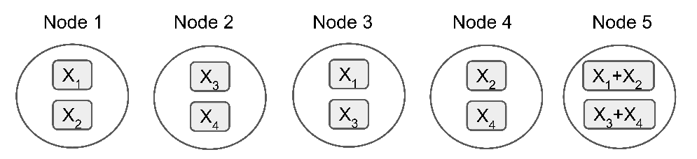
For easier description of our code construction, right after initialization, we artificially define nodes 1 and 2 as the parents of node 3 even though nodes 1 and 2 are not helpers of node 3. The reason is that the packets in node $3$ are $\{X_{1},X_{3}\}$ and they can be viewed as if node 3 has failed and got repaired from nodes 1 and 2. See Fig. 2 for illustration. Similarly, we artificially define nodes 1 and 2 as the parents of node 4 (resp. node 5) even though nodes 1 and 2 are not helpers of node 4 (resp. node 5).⁹⁹ 9 Even with the artificially defined parent-child relationship, there is no triangle after initialization. We can thus use the same induction proof to show that CA is always possible after initialization.

The regular repair operations: Suppose node $a$ fails and one other node is temporarily unavailable at time $\tau$. We run the aforementioned CA helper selection scheme to find the helpers $b$ and $c$ for node $a$. Denote the two non-helper nodes by $d$ and $e$. Each of $b$ and $c$ will send 1 packet to $a$ since $\beta=1$. The packets are constructed as follows. Step 1: Denote the two (potentially coded) packets stored in $b$ by $Y_{1}^{(b)}$ and $Y_{2}^{(b)}$. Among the three candidate packets $Y_{1}^{(b)}$, $Y_{2}^{(b)}$, and the binary sum $[Y_{1}^{(b)}+Y_{2}^{(b)}]$, node $b$ will choose one packet, call it $Z_{b}^{*}$, and send it to $a$.

Before describing how to choose $Z_{b}^{*}$, we construct two conditions based on the packets currently stored in nodes $c$, $d$, and $e$. If nodes $c$ and $d$ jointly contain 4 linearly independent packets, then we construct Condition 1 to be “$Z_{b}^{*}$ cannot be expressed as a linear combination of the two packets stored in $d$.” Otherwise, we construct Condition 1 to be “$Z_{b}^{*}$ cannot be expressed as a linear combination of the packets stored in $c$ and $d$.” Namely, depending on the coded packets stored in nodes $c$ and $d$, Condition 1 can be one of the above two different statements. Similarly, if nodes $c$ and $e$ jointly contain 4 linearly independent packets, then we construct Condition 2 to be “$Z_{b}^{*}$ cannot be expressed as a linear combination of the two packets stored in $e$.” Otherwise, we construct Condition 2 to be “$Z_{b}^{*}$ cannot be expressed as a linear combination of the packets stored in $c$ and $e$.”

After constructing the two conditions, we require the choice $Z_{b}^{*}$ to satisfy simultaneously both Conditions 1 and 2. If there is more than one choice of $Z_{b}^{*}$ satisfying both conditions, then an arbitrary one of those $Z_{b}^{*}$ will do.

Step 2: Denote the two packets stored in $c$ by $Y_{1}^{(c)}$ and $Y_{2}^{(c)}$. Among three candidate packets $Y_{1}^{(c)}$, $Y_{2}^{(c)}$, and the binary sum $[Y_{1}^{(c)}+Y_{2}^{(c)}]$, node $c$ will choose one packet, call it $Z_{c}^{*}$, and send it to node $a$. We require the packet $Z_{c}^{*}$ to satisfy simultaneously: (i) $Z_{c}^{*}$ cannot be expressed as a linear combination of $Z_{b}^{*}$ and the two packets stored in $d$; and (ii) $Z_{c}^{*}$ cannot be expressed as a linear combination of $Z_{b}^{*}$ and the two packets stored in $e$.

Once node $a$ receives $Z_{b}^{*}$ and $Z_{c}^{*}$, it stores both packets in its local memory (since $\alpha=2$).

The proof of Lemma 1 is relegated to Appendix D.

The proof of Proposition 7 is relegated to Appendix D.

Let us use an example to illustrate our construction. Suppose after initialization, node 3 fails and node 2 is unavailable. Newcomer 3 thus has to access two of the nodes $\{1,4,5\}$ for repair. Since node 1 is the parent of both nodes $4$ and $5$, the CA scheme will avoid choosing $\{1,4\}$ and $\{1,5\}$ and select helpers $\{4,5\}$ instead. Specifically, $a=3$, $b=4$, and $c=5$; and $d=1$ and $e=2$.

Since node $b=4$ stores $\{X_{2},X_{4}\}$, see Fig. 2, the three candidates for $Z_{b}^{*}$ are $X_{2}$, $X_{4}$, and $[X_{2}+X_{4}]$.

Since node $c=5$ stores $\{[X_{1}+X_{2}],[X_{3}+X_{4}]\}$ and node $d=1$ stores $\{X_{1},X_{2}\}$, these two thus contain 4 linearly independent packets. Condition 1 becomes “$Z_{b}^{*}$ cannot be any linear expression of packets $X_{1}$ and $X_{2}$, the packets in node $d$.” Similarly, since $e=2$ stores $\{X_{3},X_{4}\}$ and jointly nodes $c$ and $e$ contain 4 linearly independent packets, Condition 2 becomes “$Z_{b}^{*}$ cannot be any linear expression of packets $X_{3}$ and $X_{4}$, the packets in node $e$.” Out of the three candidates $X_{2}$, $X_{4}$, and $[X_{2}+X_{4}]$, only the coded packet $[X_{2}+X_{4}]$ can satisfy both conditions simultaneously. Therefore we choose $Z_{b}^{*}=[X_{2}+X_{4}]$.

Since node $c=5$ stores $\{[X_{1}+X_{2}],[X_{3}+X_{4}]\}$, the three candidates for $Z_{c}^{*}$ are $[X_{1}+X_{2}]$, $[X_{3}+X_{4}]$, and $[X_{1}+X_{2}+X_{3}+X_{4}]$. The choice of $Z_{c}^{*}$ thus has to satisfy simultaneously (i) $Z_{c}^{*}$ is not a linear combination of $Z^{*}_{b}=[X_{2}+X_{4}]$ and the two packets $X_{1}$ and $X_{2}$ in node $d$; and (ii) $Z_{c}^{*}$ is not a linear combination of $Z^{*}_{b}=[X_{2}+X_{4}]$ and the two packets $X_{3}$ and $X_{4}$ in node $e$. Out of the three candidates $[X_{1}+X_{2}]$, $[X_{3}+X_{4}]$, and $[X_{1}+X_{2}+X_{3}+X_{4}]$, only the coded packet $[X_{1}+X_{2}+X_{3}+X_{4}]$ can satisfy both conditions simultaneously. Therefore, we choose $Z_{c}^{*}=[X_{1}+X_{2}+X_{3}+X_{4}]$.

References

- [1] R. Ahlswede, N. Cai, S.-Y. R. Li, and R. W. Yeung, “Network information flow,” IEEE Trans. Inf. Theory, vol. 46, no. 4, pp. 1204–1216, 2000.
- [2] I. Ahmad and C.-C. Wang, “Locally repairable regenerating code constructions,” [Online]. Available: arXiv:[cs.IT].
- [3] ——, “When can helper node selection improve regenerating codes? Part I: Graph-based analysis,” [Online]. Available: arXiv:1604.08231 [cs.IT].
- [4] ——, “When can helper node selection improve regenerating codes? Part II: An explicit exact-repair code construction,” [Online]. Available: arXiv:1604.08230 [cs.IT].
- [5] ——, “When and by how much can helper node selection improve regenerating codes?” in Proc. 52nd Annu. Allerton Conf. Communication, Control, and Computing, Monticello, IL, Oct. 2014, pp. 459 – 466.
- [6] V. R. Cadambe, S. A. Jafar, H. Maleki, K. Ramchandran, and C. Suh, “Asymptotic interference alignment for optimal repair of mds codes in distributed storage,” IEEE Trans. Inf. Theory, vol. 59, no. 5, pp. 2974–2987, 2013.
- [7] A. G. Dimakis, P. B. Godfrey, Y. Wu, M. J. Wainwright, and K. Ramchandran, “Network coding for distributed storage systems,” IEEE Trans. Inf. Theory, vol. 56, no. 9, pp. 4539–4551, 2010.
- [8] R. Dougherty, C. Freiling, and K. Zeger, “Insufficiency of linear coding in network information flow,” IEEE Trans. Inf. Theory, vol. 51, no. 8, pp. 2745–2759, 2005.
- [9] P. Gopalan, C. Huang, H. Simitci, and S. Yekhanin, “On the locality of codeword symbols,” IEEE Trans. Inf. Theory, vol. 58, no. 11, pp. 6925–6934, 2012.
- [10] H. D. L. Hollmann, “On the minimum storage overhead of distributed storage codes with a given repair locality,” in Proc. IEEE Int. Symp. Information Theory (ISIT), Honolulu, HI, Jun. 2014, pp. 1041–1045.
- [11] G. M. Kamath, N. Prakash, V. Lalitha, and P. V. Kumar, “Codes with local regeneration and erasure correction,” IEEE Trans. Inf. Theory, vol. 60, no. 8, pp. 4637–4660, 2014.
- [12] G. M. Kamath, N. Silberstein, N. Prakash, A. S. Rawat, V. Lalitha, O. O. Koyluoglu, P. Kumar, and S. Vishwanath, “Explicit mbr all-symbol locality codes,” in Proc. IEEE Int. Symp. Information Theory (ISIT), Istanbul, Turkey, Jul. 2013, pp. 504–508.
- [13] L. Pamies-Juarez, H. D. L. Hollmann, and F. Oggier, “Locally repairable codes with multiple repair alternatives,” in Proc. IEEE Int. Symp. Information Theory (ISIT), Istanbul, Turkey, Jul. 2013, pp. 892–896.
- [14] D. S. Papailiopoulos and A. G. Dimakis, “Locally repairable codes,” IEEE Trans. Inf. Theory, vol. 60, no. 10, pp. 5843–5855, 2014.
- [15] N. Prakash, G. M. Kamath, V. Lalitha, and P. V. Kumar, “Optimal linear codes with a local-error-correction property,” in Proc. IEEE Int. Symp. Information Theory (ISIT), Cambridge, MA, Jul. 2012, pp. 2776–2780.
- [16] K. V. Rashmi, N. B. Shah, and P. V. Kumar, “Optimal exact-regenerating codes for distributed storage at the msr and mbr points via a product-matrix construction,” IEEE Trans. Inf. Theory, vol. 57, no. 8, pp. 5227–5239, 2011.
- [17] A. S. Rawat, O. O. Koyluoglu, N. Silberstein, and S. Vishwanath, “Optimal locally repairable and secure codes for distributed storage systems,” IEEE Trans. Inf. Theory, vol. 60, no. 1, pp. 212–236, 2014.
- [18] N. B. Shah, K. V. Rashmi, P. V. Kumar, and K. Ramchandran, “Distributed storage codes with repair-by-transfer and nonachievability of interior points on the storage-bandwidth tradeoff,” IEEE Trans. Inf. Theory, vol. 58, no. 3, pp. 1837–1852, 2012.
- [19] ——, “Interference alignment in regenerating codes for distributed storage: Necessity and code constructions,” IEEE Trans. Inf. Theory, vol. 58, no. 4, pp. 2134–2158, 2012.
- [20] K. W. Shum and Y. Hu, “Cooperative regenerating codes,” IEEE Trans. Inf. Theory, vol. 59, no. 11, pp. 7229–7258, 2013.
- [21] C. Tian, “Characterizing the rate region of the (4, 3, 3) exact-repair regenerating codes,” Selected Areas in Communications, IEEE Journal on, vol. 32, no. 5, pp. 967–975, 2014.
- [22] D. B. West, Introduction to graph theory. Prentice Hall Upper Saddle River, NJ., 2001, vol. 2.
- [23] Y. Wu, “Existence and construction of capacity-achieving network codes for distributed storage,” IEEE J. Select. Areas Commun., vol. 28, no. 2, pp. 277–288, 2010.