Physical Review A 91, 062309 (2015)
Universal quantum simulation with prethreshold superconducting qubits: Single-excitation subspace method
Abstract
Current quantum computing architectures lack the size and fidelity required for universal fault-tolerant operation, limiting the practical implementation of key quantum algorithms to all but the smallest problem sizes. In this work we propose an alternative method for general-purpose quantum computation that is ideally suited for such “prethreshold” superconducting hardware. Computations are performed in the -dimensional single-excitation subspace (SES) of a system of tunably coupled superconducting qubits. The approach is not scalable, but allows many operations in the unitary group SU() to be implemented by a single application of the Hamiltonian, bypassing the need to decompose a desired unitary into elementary gates. This feature makes large, nontrivial quantum computations possible within the available coherence time. We show how to use a programmable SES chip to perform fast amplitude amplification and phase estimation, two versatile quantum subalgorithms. We also show that an SES processor is well suited for Hamiltonian simulation, specifically simulation of the Schrödinger equation with a real but otherwise arbitrary Hamiltonian matrix. We discuss the utility and practicality of such a universal quantum simulator, and propose its application to the study of realistic atomic and molecular collisions.
pacs
03.67.Lx, 85.25.CpI INTRODUCTION AND MOTIVATION
I.1 The promise of quantum computation
A universal quantum computer, if one could be built, would transform information technology by providing vastly increased computational power for certain specialized tasks, such as quantum simulation [1, 2, 3, 4, 5] and prime factorization [6, 7]. Superconducting electrical circuits operating in the quantum regime [8, 9] have emerged as an extremely promising platform for realizing a large-scale, practical machine. Yet the quantum algorithms actually demonstrated to date—with any architecture—have been limited to only tiny, few-qubit instances [10, 11, 12, 13, 14, 15, 16, 17, 18, 19, 20, 21, 22, 23, 24, 25, 26, 27, 28, 29, 30, 31, 32, 33]. In superconducting circuit or circuit QED implementations, which benefit from the inherent scalability of modern solid-state electronics, this barrier in qubit number does not reflect any limitation of the underlying device fabrication or infrastructure requirements, but rather that larger problem sizes would also require longer computations and hence additional coherence. Quantum algorithms typically have (uncompiled) circuits that are spatially narrow but temporally very deep. In this work we propose an alternative approach to superconducting quantum information processing that allows one to circumvent this restriction and realize much larger computations within the available coherence time.
A general-purpose quantum computer that is useful for practical applications must, of course, be error corrected and scalable. The standard model of an error-corrected quantum computer is the gate-based fault-tolerant universal quantum computer, where “errors” acting on all device components and at any step during the computation can be corrected as long as they are weak enough—below an error threshold [34, 35, 36]—and not highly correlated in space or time [37, 38, 39, 40]. Scalability means that the number of physical qubits required to perform a particular computation—the physical volume of the quantum computer—scales as a polynomial function (preferably linear) of the problem size. It also means that it is actually possible, in practice, to add more qubits.
A realistic picture of an error-corrected superconducting quantum computer based on the surface code [41, 42] is beginning to emerge [43]. The surface code is the most practical, best performing fault-tolerant approach known to date, and is especially amenable to implementaion with superconducting circuit technology. However, the resources required for a practical machine are considerable: Fowler et al. [43] estimated that factoring a 2000-bit number would require about physical qubits, using Beauregard’s modular exponentiation [44] and a surface code quantum computer operating at fidelity. If there was no decoherence or noise, and no errors of any kind to correct, then it would be possible to factor an -bit number with the Beauregard algorithm using only ideal qubits, or 4003 ideal qubits in the case considered. Thus, error correction imposes a physical qubit overhead of . Note that in quantifying the error-correction overhead here we distinguish between ideal (error free) qubits—the fictional entities usually appearing in quantum algorithms—and logical qubits, which must also include the many additional ancillas necessary for fault-tolerant gate implementation. Similarly, You et al. [45] estimated that it would take about physical qubits to calculate the ground state energy of a 100-spin transverse-field Ising model to accuracy using the same -fidelity surface code quantum computer. This well known statistical mechanics model maps especially well to a quantum computer, and for spins on a line would require only ideal qubits for a calculation of the ground state energy (using iterative phase estimation). So the physical/ideal ratio in this quantum simulation example is , the same as for factoring. Therefore we expect that, in practice, surface code error correction will impose an overhead of
| (1) |
where we have allowed for future optimization and other improvements. Crudely, a factor of about 10 in the overhead estimate comes from replacing ideal qubits with enough logical qubits to both encode those ideal qubits and to distill the auxiliary states needed to perform fault-tolerant operations on them, and a factor of about comes from replacing each logical qubit with enough physical qubits to enable a sufficiently long computation.
I.2 Prethreshold quantum computation
The complexity of building even a small fault-tolerant universal quantum computer suggests that this objective may take some time to achieve. In the meantime, experimental quantum information processing is limited to either the very small problem sizes discussed above, or to nonuniversal approaches such as analog quantum simulation [5, 46, 47, 48], quantum annealing [49, 50], or other special-purpose methods [51, 52]. In this work we label any quantum computation without an error-corrected universal quantum computer as prethreshold, referring to the threhold theorems of fault-tolerant quantum computation, because exceeding a fidelity threshold is a necessary condition for large-scale error correction.
Table 1 compares three broad approaches to quantum computation with prethreshold hardware: Small system refers to gate-based computations with a few qubits, which have been used to test fundamental concepts of quantum information processing, demonstrate hardware functionality, and assess qubit and gate performance. The SES method is also general purpose, but should enable quantum speedup (this is discussed below). However neither approach is scalable. Analog quantum simulation and other scalable, special-purpose approaches trade universality for a faster route to speedup.
The SES quantum computer described in this work is universal in the sense that it can implement any gate-based algorithm or quantum circuit. As a simulator it can directly emulate any (real) Hamiltonian, including time-dependent Hamiltonians. When we refer to a simulated Hamiltonian in this context we mean a Hamiltonian written in some basis—a real, symmetric matrix with no special structure. We assume that the Hamiltonian matrix to be simulated has been specified externally, as is typically the case when using a classical computer. The SES processor solves the Schrödinger equation defined by this Hamiltonian.
| small system | SES method | analog QS/spec purp | |
|---|---|---|---|
| scalable | |||
| universal | |||
| speedup | |||
| arb accuracy | |||
| arb runtime |
The superconducting SES method introduced here has features in common with the single-photon protocols of Reck et al. [53] and Cerf et al. [54], as both use only one excitation, and therefore do not utilize genuine entanglement. The optical realization uses a recursive algorithm to first decompose a given unitary of interest into a sequence of SU(2) beam-splitter transformations. This decomposition determines an arrangement of beam splitters, phase shifters, and mirrors, that will unitarily transform input ports (optical modes) to output ports according to the desired . However, the superconducting realization is better suited for quantum simulation than the optical approach because the Hamiltonian is directly programmed. In particular, to optically simulate Schrödinger evolution under a given Hamiltonian matrix , one would have to first compute the evolution operator on a classical computer, and then decompose it into beam-splitter transformations, but avoiding the classical computation of (or the time-ordered exponential if is time dependent) is the motivation for the quantum computation in the first place [55]. Neither the superconducting SES nor the single-photon optical approaches are scalable—they both require exponential physical resources—and should not be considered as viable alternatives to the standard paradigm of error-corrected universal quantum computation. But they are both suitable prethreshold methods.
II QUANTUM COMPUTATION IN THE SES
II.1 Hardware model: The programmable SES chip
Consider the following model of an array of coupled superconducting qubits,
| (2) |
written in the basis of uncoupled-qubit eigenstates. Here and
| (3) |
The are qubit transition energies and the are qubit-qubit interaction strengths; both are assumed to be tunable. (Factors of are suppressed throughout this paper.) is a real, symmetric matrix with vanishing diagonal elements. We also require microwave pulse control of at least one qubit, and simultaneous readout (projective measurement in the diagonal basis) of every qubit. The model (2) describes a fully connected network or complete graph of qubits, which we refer to as an SES processor. This should be contrasted with local quantum computer models that have coupling only between nearby qubits (nearest neighbors, for example). The SES method can be applied with a wide variety of qubit-qubit interaction types (see Appendix A), but without loss of generality we restrict ourselves here to the simple coupling of (2). Alternatively, tunably coupled resonators (with tunable frequencies) can be used instead of qubits [56]. Although we assume an architecture based on superconducting circuits (or circuit QED), the SES method might apply to other future architectures as well.
The quantum computer model (2) might be considered unscalable, because of the tunable coupling circuits and wires, a position that we also adopt here. In gate-based universal quantum computation, the fully connected and local quantum computer models are equivalent in the sense that any quantum circuit implemented by a fully connected quantum computer can be implemented by a local quantum computer after adding chains of SWAP gates, which only introduce polynomial overhead. However, this equivalence is restricted to the standard gate-based approach and does not apply here.
Superconducting qubits have been reviewed in Refs. [8] and [9]. Although the model (2) can be realized with several qubit designs, the transmon qubit [57] currently has the best performance [58, 59, 60, 61]. For concreteness we assume a qubit frequency in the range of to and coupling strength in the range to . An -qubit SES processor also requires coupler circuits and the associated wires or waveguides. A variety of tunable couplers can be used for this purpose. Here we consider a modification of the tunable inductive coupler developed by Chen et al. [61] for superconducting Xmon qubits; this design has been demonstrated to implement tunability without compromising high coherence. Our modification replaces the direct electrical connection of each qubit to a coupler circuit wire with an inductive coupling to the wire, which scales better. An SES chip layout that avoids excessive crossovers is illustrated in Fig. 1. The tunable interaction strength for this coupler design is derived in Appendix B.

II.2 Single-excitation subspace
The idea we explore in this paper is to perform a quantum computation in the -dimensional single-excitation subspace of the full -dimensional Hilbert space. This is the subspace spanned by the computational basis states
| (4) |
with We call the set of the SES basis states. It is simple to prepare the quantum computer in an SES basis state from the ground state , and it will remain there with high probability if the following conditions are satisfied:
- 1.
The coupling strengths are much smaller than the , which is usually well satisfied in superconducting circuits.
- 2.
Single-qubit operations such as and rotations about the or axes are not used during the computation. However, rotations are permitted and are very useful (these can be implemented as rotations, which do not require microwaves). rotations about or can be used to prepare SES basis states from the system ground state .
- 3.
The quantum computation time is significantly shorter than the single-qubit population relaxation time .
II.3 SES Hamiltonian
The advantage of working in the SES can be understood from the following expression for the SES matrix elements of model (2), namely
| (7) |
Because the diagonal and off-diagonal elements are directly and independently controlled by the qubit frequencies and coupling strengths, respectively, we have a high degree of programmability of the SES component of the quantum computer’s Hamiltonian. This property allows many -dimensional unitary operations to be carried out in a single step, bypassing the need to decompose into elementary gates, and also enables the direct quantum simulation of real but otherwise arbitrary time-dependent Hamiltonians. However, we have some restrictions:
- 1.
is always real, whereas the most general Hamiltonian matrix is complex Hermitian. The experimentally available control parameters, consisting of qubit frequencies and coupling strengths, are sufficient to control the independent parameters of an real symmetric matrix.
- 2.
There are experimental limitations on the range of values that the and can take. We define to be the magnitude of the largest coupling available in a particular experimental realization; a current realistic value is about .
We will leave the discussion of possible generalizations to complex SES Hamiltonians for future work. The limitations on the ranges of the and do not, by themselves, limit the class of Hamiltonians that can be simulated, because a model Hamiltonian intended for simulation is first rescaled to conform to that of the SES chip (this is explained below).
It will be useful to refer to a “typical” SES Hamiltonian , which we assume to have the following properties: is a real, symmetric matrix with each element taking values in the range to . This form follows from (7) after removing an unimportant term proportional to the identity matrix,
| (8) |
where is a convenient (possibly time-dependent) reference frequency. Then we assume that the qubit frequencies can be tuned within of , and we assume that the couplers can be tuned between to . A possible choice for is the mean qubit frequency .

It will also be useful to consider the statistical properties of an ensemble of typical SES matrices. We can always write a time-independent SES Hamiltonian in the standard form
| (9) |
where is real symmetric matrix with every element satisfying
| (10) |
We define a real random matrix ensemble of dimension as follows: The diagonal elements are independent random variables , each uniformily distributed between and . The elements are independent random variables also uniformily distributed between and . The remaining elements are fixed by the symmetry requirement. The standard deviation of each element is

The first property we study is the mean spectral bandwidth of , the difference between the largest and smallest eigenvalues. Let be the ordered eigenvalues of . From the Wigner semicircle law [63] we expect that, in the large limit,
| (11) |
where the overbar denotes averaging over the ensemble defined above. The bandwidth of typical SES states in an -qubit processor therefore scales at large as
| (12) |
In Figs. 2 and 3 we plot the simulated bandwidth of as a function of , and compare the simulation data with the asymptotic form (11). From Fig. 2 we conclude that for modest SES matrix sizes,
| (13) |
The second property we study is the mean level spacing of . Let
| (14) |
be the mean spacing between adjacent eigenvalues. Averaging (14) over the ensemble defined above, we expect that in the large limit
| (15) |
In Fig. 4 we plot the simulated average level spacing of as a function of , and compare the simulation data with the asymptotic form (15). From Fig. 4 we conclude that for modest SES matrix sizes,
| (16) |
The results (13) and (16) give two relevant energy scales present in a typical SES spectrum.
Any unitary quantum circuit or operation acting on qubits can be mapped to and implemented on an SES chip with qubits (this exponential growth of is what makes the SES method unscalable). We can say that the SES processor simulates the -qubit system, with the advantage of being able to perform multi-qubit operations in a single step. This feature provides the computational advantage of the SES approach and is illustrated throughout this paper. It will be useful to specify an explicit one-to-one mapping between the bases of the associated Hilbert spaces, which we take to be
| (17) |
The left-hand-sides are the standard computational basis states of the simulated -qubit system (not to be confused with the computational basis states of the -qubit SES processor). Similarly, any unitary quantum circuit or operation acting on -level qudits can be mapped to and implemented on an SES processor with qubits; the natural mapping is a straightforward generalization of (17).

The operation of a real SES chip will be nonideal, and it is important to consider the effects of decoherence and other errors on its performance. This is discussed in detail in Sec. IV. The main conclusion is that although decoherence and unitary control errors do limit the accuracy of an SES computation or simulation, the effects of decoherence are much less restrictive here than with the standard gate-based approach (hence the ability to implement larger problem sizes). In practice, the complexity of fabricating a large programmable SES chip will likely limit its application before decoherence does.
III APPLICATIONS OF THE SES METHOD
III.1 Uniform state preparation
Our first example will be to generate the entangled state (6) in a single step: Consider the real Hamiltonian
| (18) |
where
| (19) |
The Hamiltonian (18) describes a graph where qubit 1 is symmetrically coupled to all other qubits, which are themselves uncoupled (a star network). The case of qubits is shown in Fig. 5.
The SES chip is initially prepared in basis state . Only two eigenfunctions—let’s call them —have overlap with , so the evolution is effectively a two-channel problem. The spectrum is as follows: States have energy ; all other eigenfunctions are degenerate with . Evolution for half a period corresponding to the splitting , namely
| (20) |
leads to the desired operation
| (21) |
apart from a phase. This can be implemented in a few ns with superconducting circuits.

We would like to make a few remarks that apply to this application, as well as to many others: First, the magnitude of the interaction strength used in (18) is arbitrary; any convenient interaction strength satisfying is sufficient. To make the operation as fast as possible, however, we have choosen . Second, it is not necessary to use a time-independent interaction strength. Any single-step “pulse sequence” of the form
| (22) |
with
| (23) |
and a constant (time-independent) matrix, satisfies an area theorem
| (24) |
where
| (25) |
and is the time-ordering operator. The identity (24) implies that any time-dependent coupling satisfying (25) can be used, simplifying experimental implementation.
III.2 Grover search algorithm
Next we show how to use a programmable SES chip to implement the Grover search algorithm [64], which introduced the powerful amplitude amplification technique that has led to speedup for many other algorithms. Grover’s procedure for a single marked state in a database of size is
| (26) |
Here
| (27) | |||||
is a unitary operator that performs an inversion about the average,
| (28) |
is the oracle, a diagonal matrix with the th element equal to and the others equal to , and is the uniform superposition (6).
The operator (27) can be implemented in a single step by using the SES Hamiltonian with
| (29) |
for a time
| (30) |
This leads to the desired operation
| (31) |
up to a phase factor.
The oracle (28) can be simply generated by a rotation on qubit . This rotation can be implemented as a rotation, which does not require microwaves. Each iteration of the amplitude amplification can therefore be implemented in just two steps, for any , allowing even small SES chips to perform computations that would otherwise require thousands of elementary gates.
III.3 Eigenvalue estimation
Next we show how to use a programmable SES processor to implement energy eigenvalue estimation, an application of the important phase estimation algorithm [65, 66, 67] that is used in many other applications. This example also illustrates how to translate an algorithm expressed in quantum circuit language to an SES protocol.
The eigenvalue estimation procedure calculates an -bit estimate of the phase of the eigenvalue accumulated by an eigenfunction under the action of If the evolution time is chosen to satisy the eigenvalue (assumed to be positive) can be calculated from . To reduce the number of required qubits we use the iterative phase estimation circuit [68] shown in Fig. 6, which uses only a single ancilla. As the number of desired bits of precision increases, one either performs a longer quantum computation—reusing the eigenfunction —or performs computations in series, each requiring an eigenfunction preparation step.
The algorithm measures bits of one at a time, beginning with the least significant bit , and working backwards to the most significant bit . Each step (except for the first) uses knowledge of the previously measured bits. We denote the bit being measured in a given step by , with The circuit for step is shown in Fig. 6, where the rotation angle is
| (32) |
which depends on the values of the previously measured bits .

The main practical difficulty with prethreshold applications of phase estimation is implementation of the
| (33) |
operation, which typically requires a Trotter approximation (and, in addition, a sparse Hamiltonian). However, the SES method allows any controlled unitary
| (34) |
to be implemented in a single step when can (which is possible when is symmetric). To see this, assume that , where is a real matrix, and write the matrix (34) as
| (35) |
where is the identity matrix and where we take the first qubit to be the control. Next map the -dimensional Hilbert space to the SES processor according to
| (36) |
The operation (34) can therefore be written as
| (37) |
which can be implemented by an SES processor in a single step. The elements and on the right-hand-side of (37) are each matrices, with the zero (null) matrix.
We turn now to the SES eigenvalue estimation protocol: Let be a real model Hamiltonian on which we wish to perform phase estimation, and denote the basis of by . The SES implementation requires qubits. The first objective in the protocol is to prepare the initial state
| (38) |
of Fig. 6, where is an eigenfunction of . We will perform the state preparation adiabatically, which is restricted to states of minimum or maximum energy; here we prepare the ground state of and estimate the ground state energy .
Adiabatic ground state preparation is usually implemented by programming a convenient initial Hamiltonian that does not commute with , relaxing into the ground state of , and then slowly changing the system Hamiltonian from to . However, in the SES approach it is necessary to use nonequilibrium adiabatic evolution, because the physical ground state is outside the SES. The processor is initially prepared in the basis state . The next step is to produce the SES state equivalent to
| (39) |
which, according to the map (36), is
| (40) |
Note that (40) is a uniform superposition of the first half of SES basis states. To prepare this we use a variation of (21), namely
| (41) |
where
| (42) |
is a block-diagonal Hamiltonian. Here is an matrix of the form (19), and is the zero matrix. The operation time in (41) is
| (43) |
This completes the preparation of the input (40) to the adiabatic evolution stage.
At the beginning of the adiabatic evolution stage we program the SES Hamiltonian to be
| (44) |
where is an Hamiltonian with the following properties:
- 1.
is real.
- 2.
.
- 3.
The ground state of is the uniform superposition state (40).
- 4.
The ground state is separated from the other eigenstates by an energy gap that is a nondecreasing function of .
A possible choice when is a power of two is the “transverse field” Hamiltonian
| (45) |
However, the explicit matrix forms of (45) for large are complicated and the tensor-product structure is somewhat artifical for our purposes. Instead we use
| (46) |
where is an matrix of the form (29). The initial Hamiltonian (46) has eigenvalues
| (47) |
where . The ground state is
| (48) |
with energy The remaining eigenfunctions are degenerate with energy .
At later times the SES Hamiltonian is varied as
| (49) |
Here
| (50) |
is a positive constant that ensures that can be programmed into the SES processor. This stage of the protocol is standard: In the long adiabatic limit, the processor will be found at in the desired state (38) with high probability.
Next we implement the SES equivalent of the circuit given in Fig. 6, beginning with the Hadamard gate
| (51) |
which we write as
| (52) |
where
| (53) |
Then we have
| (54) |
where is the diagonal matrix
This leads to
| (71) |
where is the Hamiltonian , with
| (72) |
and
| (73) |
The controlled-evolution step has been discussed above in (34) through (37). Applying this result to the operation (33) leads to
| (74) |
Here and are matrices, with the model Hamiltonian, which we assume to be real. Now let be defined as in (50). Then
| (75) |
where
| (76) |
To perform the controlled-evolution operation, the Hamiltonian in (76) is to be programmed into the SES processor for a time .
Finally, we implement the rotation
| (77) |
where
| (78) |
This operation can be generated by applying the Hamiltonian for a time
The final stage of the eigenvalue estimation protocol is the SES equivalent of ancilla measurement (see Fig. 6), resulting in the observed value . One way to do this is to perform a simultaneous projective measurement of every qubit in the SES processor. If the excitation at iteration is observed to be in qubit , we conclude that
| (79) |
This result follows from the correspondence (36). The disadvantage of this naive measurement protocol is that it fully collapses the SES wave function, so the eigenfunction needs to be re-prepared before the next iteration.
A simple variation of this protocol, however, avoids the state re-preparation step about half the time: Here we simultaneously measure only the first qubits. In this case we might observe the excitation to be in qubit , or we may not find it at all. Then we conclude that
| (80) |
If the measurement fully collapses the state, and we must re-prepare the eigenfunction . But if we have learned only that the excitation is in the subspace spanned by
| (81) |
which yields no information about .
It is possible to avoid the eigenfunction re-preparation step altogether by using an example of the ancilla-assisted SES method: Here we couple an -qubit SES processor to an ancilla qubit, with a degree of connectivity that depends on the application. (The measurement application requires coupling to qubits.) Alternatively, we can regard one of the qubits in a fully connected array of qubits as an ancilla. The essential point is that the device now explores the single-excitation and double-excitation subspaces. The only disadvantage of this measurement protocol is that it requires steps per iteration.
The idea is to measure the multi-qubit operator
| (82) |
which projects qubits into a state of definite parity. If at iteration the eigenvalue of (82) is observed to be , the single excitation is in the subspace spanned by and we conclude that . If the eigenvalue is , the excitation is in the space spanned by and we conclude . The measurement of the operator (82) can be carried out with a single ancilla qubit using the circuit given in Fig. 7.

It is useful to discuss the nonscalability of the SES method in the context of the eigenvalue estimation application. Typically is exponentially large in the number of particles, making classical simulation impractical. An ideal (error-free) quantum computer would require only qubits to run the phase estimation circuit of Fig. 6. However, the large circuit depths required for the controlled evolutions have limited prethreshold applications to very small examples. The SES implementation requires qubits, but can perform the controlled evolutions in a single step.
III.4 Schrödinger equation solver for time-independent Hamiltonian matrices
Next we consider the problem of wave function propagation by a real but otherwise arbitrary time-independent Hamiltonian ,
| (83) |
This application, and especially its time-dependent extension discussed below, play to the strengths of the SES chip and suggest a useful prethreshold computational tool. We assume that is a real, symmetric matrix, and we call the model Hamiltonian. Here is the length of simulated time (for example, the duration of some physical process). To map this problem to an SES processor we first find the smallest positive constant such that every matrix element of
| (84) |
is between and . Here is the identity matrix. When we are “compressing” the model Hamiltonian down to that of the SES chip, whereas when we are expanding it. Such a rescaling is required because the characteristic energy scales of the model and SES chip are usually different. With the SES processor we then perform the equivalent evolution
| (85) |
where
| (86) |
The total time required to perform a single run of the quantum computation is therefore
| (87) |
where is the qubit measurement time. For superconducting qubits we can assume to be about [69], which includes the time needed for classical post-processing. (Note that the shortest high-fidelity readout time demonstrated to date, including resonator ring-down time, is closer to [70]. The faster “catch-disperse-release” protocol of Ref. [69] has not yet been demonstrated.)
A single run of the quantum computer (with readout) simulates a single repetition of an experiment: Initialization, Schrödinger evolution, and measurement. It is important to emphasize that such a protocol implements a weak simulation, providing a single sample from the distribution of possible measurement outcomes, not the probability distributions themselves as is normally computed classically. (This limitation is not specific to the SES method and applies to state propagation with an error-corrected universal quantum computer as well.) For some applications the distinction between weak and strong simulation might be minor. However in other cases it is necessary to estimate the occupation probabilities accurately. We discuss the runtime overhead for strong SES simulation below in Sec. III.6.
How long does a classical simulation of (83) take? This of course depends on the model Hamiltonian (including its dimension and spectral norm), the value of , and the classical processor and simulation algorithm used. To assess the possibility of quantum speedup, however, it is sufficient to find the minimum time required to classically simulate a given run of an ideal SES processor, with a “typical” SES Hamiltonian (a real random symmetric matrix with all entries between and ), and significantly less than the coherence time. For this analysis we consider the case
| (88) |
The total quantum computation time (87) in this example is therefore about
| (89) |
We have studied the classical simulation runtime for this problem, comparing, on a single core [71], three standard numerical algorithms:
- 1.
State propagation via Hamiltonian diagonalization. For a given , the unitary matrix of its eigenvectors and diagonal matrix of its eigenvalues are first computed. Then we numerically compute the product
(90) where is the initial state.
- 2.
Matrix exponentiation via Padé approximation with scaling and squaring [72]. Here we directly compute and then multiply by .
- 3.
Krylov subspace projection [73]. In this case the product itself is directly calculated.

Figure 8: (color online) Classical simulation runtime on a single core [71] versus matrix dimension , in seconds. Here the computational task is solution of the Schrödinger equation with a time-independent Hamiltonian by matrix diagonalization. Data (circles) were determined by averaging the runtimes over 1000 random instances of . The solid line is the function ; the scaling becomes at larger . The runtime for a Hamiltonian is about .
In all cases we assume an initial state of the form
| (91) |
which corresponds to a single SES basis state, and we average the computation times over 1000 random instances of . Although the three methods have similar speed and accuracy for the particular problem simulated here, the matrix diagonalization method was the fastest, followed by matrix exponentiation. We also tested Runge-Kutta integration and matrix exponentiation via Chebychev polynomial expansion [74], which were not competitive with the above methods for the specific application considered. In Fig. 8 we plot the measured single-core runtimes for the optimal classical algorithm (Hamiltonian diagonalization) versus matrix dimension . We observe that the quantum simulation time (89) is much shorter than all of the single-core runtimes considered.
Our objective is to achieve speedup relative to a state-of-the-art supercomputer, not a single core. The classical simulation runtime should then be evaluated on a supercomputer, using an optimally distributed parallel algorithm. However, we can bound the parallel performance by using the single-core result and assuming perfect parallelization efficiency: We approximate a petaflop supercomputer by gigaflop cores, and conclude that the classical runtime can be no shorter than times the single-core time. (This is a conservative estimate because high parallelization efficiency is not expected for problem sizes smaller than the number of cores.) We therefore conclude that, for this particular state propagation application, the classical simulation runtime is no shorter than
| (92) |
while the quantum simulation can be performed in a few hundred nanoseconds. The breakeven dimension according to (92) is about qubits. This is quite large given the full connectivity requirement, and it is not known whether such a device could be built in practice. However the breakeven dimension in the time-dependent case (discussed below) is considerably smaller.
In our estimate of the classical simulation runtime we have not included the time needed to store the Hamiltonian matrix in memory or perhaps compute it from a separate procedure. Similarly, for the quantum simulation time estimate we have not included the time required to send the controls to the qubits and couplers before the simulation. Furthermore, not every simulation will exhibit a speedup; this depends on the particular simulated Hamiltonian and the simulated time duration .
An interesting aspect of the Schrödinger equation solver is that the complexity is O(1): The quantum simulation time is independent of . This implies that the SES method yields an exponential speedup for this application. However such complexity considerations are probably not meaningful given that the method is not scalable.
III.5 Schrödinger equation solver for time-dependent Hamiltonians: Simulation of molecular collisions
Finally, we discuss what is perhaps the most interesting application of the SES method known to date, the solution of the Schrödinger equation with a time-dependent Hamiltonian. This is a straightforward generalization of the time-independent case, but we expect the time-dependent case to be more useful in practice. In this section we provide a detailed example of time-dependent Hamiltonian simulation with a small SES chip.
Time-dependent Hamiltonian simulation is implemented by varying the SES matrix elements (7) according to some protocol, which can be done with nanosecond resolution. This does not require any additional runtime, the time complexity is still constant, and the total quantum simulation runtime for a evolution is again given by (87). Although the classical runtime is problem specific, we can again assess the possibility of speedup by estimating the time required to classically simulate an ideal SES processor, in this case with all matrix elements varying on a nanosecond timescale. There are two types of numerical simulation algorithms we consider:
- 1.
Runge-Kutta integration. Here we solve the system of coupled ordinary differential equations
(93) Although the Runge-Kutta runtime is slower than diagonalization for a time-independent Hamiltonian, it does not slow down significantly when is time dependent.
- 2.
Time slicing combined with diagonalization. This algorithm is based on an approximate decomposition of the time-dependent problem into a sequence of constant-Hamiltonian intervals, each of width . The time must be significantly smaller than the characteristic timescale of matrix element variation, for example . Then
(94) time slices are required, and the classical runtime using this approach will be approximately times longer than (92). For the evolution, .
We find that Runge-Kutta integration is the fastest approach for the specific problem considered here. In Fig. 9 we plot the measured single-core runtimes for the optimal classical algorithm (Runge-Kutta integration) versus matrix dimension . Bounding the performance of this algorithm on a petaflop supercomputer by including a factor of (recall discussion from Sec. III.4), we conclude that for this application the classical simulation runtime is no shorter than
| (95) |
while the quantum simulation can be performed in a few hundred nanoseconds. The breakeven dimension according to (95) is around qubits. As expected, this value is much smaller than the breakeven in the time-independent case. An SES Schrödinger equation solver of modest size might be able to achieve quantum speedup relative to a petaflop supercomputer.

We turn now to a detailed example of time-dependent Hamiltonian simulation with a small programmable SES chip. One particularly interesting application of the method is to the quantum simulation of atomic and molecular collisions. Collisions are especially well suited for SES simulation because they typically involve modest Hilbert spaces—tens to thousands of channels—and in the time-dependent formulation involve Hamiltonians that are naturally bounded in time. In particular, the initial and final asymptotic Hamiltonians for neutral scatterers are diagonal (in the adiabatic basis), whereas the off-diagonal elements rapidly turn on and then off during the collision itself, inducing transitions between the channels. Although the Born-Oppenheimer potential energy surfaces used here do require a classically inefficient electronic structure precomputation, the largest potential energy surface calculations [75, 76] are far ahead of the largest classical collision simulations performed to date [77, 78, 79]. SES implementation of the semiclassical Born-Oppenheimer problem therefore has the potential to push molecular collision simulations to new unexplored regimes. (We note that there are related chemical reaction simulation methods developed by Lidar et al. [80] and by Kassal et al. [81] that do not require a precomputed potential surface, but these require an error-corrected quantum computer to implement and are not prethreshold methods.) Another useful feature of the scattering application is the convenient mapping of each molecular channel to a single SES basis state, which is possible because of the similar way initial states are prepared and final states measured in both the processor and a collision experiment. We also find that the atomic physics time and energy scales turn out to map nicely to that of superconducting qubits after optimal rescaling.

To illustrate this application we consider a three-channel Na-He collision (an unpublished preliminary account of this application is given in Ref. [82]). The three channels included in our model and their correspondence with SES basis states are
| (96) |
and
| (97) |
The square brackets indicate the molecular structure of the channels. In this model, the helium atom remains in its electronic ground state during the collision (the excitation energies of its excited states are too high to be relevant here), whereas sodium can be excited from its ground state to either of two excited states, both denoted by . In the physical system, the channels (96) and (97) have additional degeneracies, including spin degeneracies, but they do not affect the collision probabilities calculated here. Precomputed Born-Oppenheimer energies and nonadiabatic couplings of the Na-He system [83] are stored for fixed values of the internuclear distance , and we make a standard semiclassical (high energy) approximation and assume that the scatterers follow a straight-line trajectory. Then, for an impact occuring at a time , the internuclear separation varies according to
| (98) |
where is the initial relative velocity and the impact parameter of the collision. The relative velocity is related to the collision energy in the center-of-mass frame through where is the reduced mass. The procedure outlined in Appendix C then leads to the scattering Hamiltonian shown in Fig. 10.

In Fig. 11 we plot the probabilities for the Na-He system to be found in channel after being initially prepared in channel 1, the ground state. The final values are the probabilities for an elastic () or inelastic () collision with a given and , which we find to be
| (99) |
To simulate this process with a programmable SES chip we must first rescale the physical or model Hamiltonian so that it fits on the SES processor. Doing this optimally is critical to the utility of any time-dependent simulation so we will discuss it in some detail: Suppose for the moment that our model Hamiltonian is given by a time-independent real symmetric matrix . Dividing by any positive constant while rescaling the evolution time by the same factor obviously leaves the dynamics invariant. Because we want the quantum simulation to be as fast as possible, we choose the smallest value of that makes compatible with the SES processor (every matrix element of is between and ). As mentioned above, if we are compressing the model’s energy scales to fit on the SES chip, whereas if we are expanding them. This naive approach to rescaling, however, does not take advantage of the fact that we can always shift by a constant (which changes the corresponding states by a phase factor that we do not measure). Including this gauge transformation results in the rescaling used above in (84). The time required to simulate an evolution of duration is simply given by (86), but now we will go further and regard (86) as giving the linear relationship between the simulated and physical times during a process. To generalize this construction to a time-dependent model Hamiltonian we first compute the mean of its diagonal elements,
| (100) |
and then find, at each time the smallest positive such that every matrix element of
| (101) |
is between and . The function defines the resulting nonlinear relation between the physical and simulated times according to
| (102) |
Equation (101) gives the simulated Hamiltonian as a function of the physical time , and (102) is then inverted to find the desired , which in turn is programmed into the SES chip.
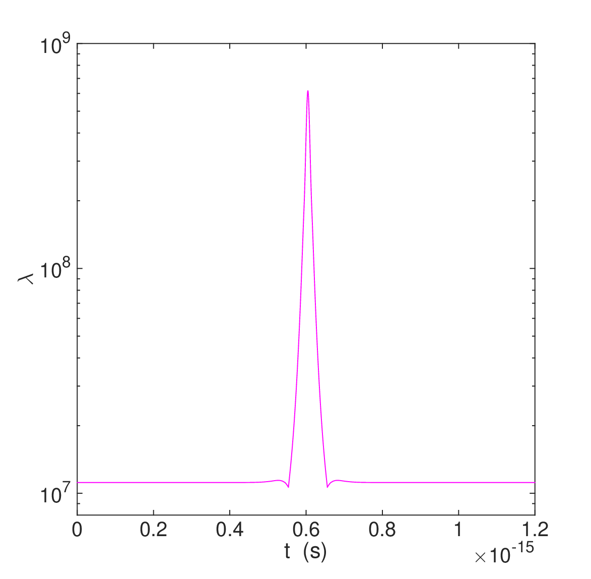

Applying this procedure to the Na-He collision problem results in the rescaling function shown in Fig. 12, and the nonlinear time relationship shown in Fig. 13. We note that the nonlinear energy/time rescaling protocol is extremely effective at mapping this atomic physics problem to the SES processor, allowing a single run of the simulation (excluding measurement) to be completed in about . The function shown in Fig. 12 assumes ; if this is increased to the simulation is completed in . It is important to emphasize that any positive piecewise continuous function defines a mathematically valid energy/time rescaling, and that the specific form used in practice should be determined by hardware considerations, such as qubit coherence times and control pulse bandwidth. In particular, can be chosen to bound both the magnitude of the SES matrix elements and their rates of change, but we will not pursue this variation here.

Use of the rescaling function given in Fig. 12 leads to the SES matrix elements shown in Fig. 14, which bear no resemblance to those of Fig. 10. The corresponding scattering probabilities during the simulation are shown in Fig. 15. Compared with Fig. 11, we see that the dynamics near the moment of collision are rescaled to occupy most of the simulation. The final scattering probabilities are the same as in Fig. 11 and are given in (99).

III.6 Strong quantum simulation
As we have emphasized, a single run of the SES chip provides a single sample from the distribution of possible measurement outcomes—a weak simulation—not the probability distributions themselves as is normally computed classically. If the objective is to perform a strong simulation and hence estimate the basis state occupation probabilities , it is necessary to repeat the simulation and readout many times. In this section we discuss the runtime overhead for strong SES simulation. (The objective considered is that of measuring occupation probabilities, not probability amplitudes.)
Suppose that after some simulation we want to measure the occupation probability of one qubit in the SES chip. We do this by performing the simulation times, after each repetition measuring the qubit in the diagonal basis and observing . The estimate
| (103) |
for will have a sampling error (standard error of the mean) given by
| (104) |
For example, to ensure that the sampling error is smaller than 1%, it is sufficient to repeat the simulation 2500 times.
The overhead is a worst-case estimate for a 1% sampling error. If is known to be small (or close to 1), fewer repetitions are required. However in this work we restrict ourselves to the case where measuring is the objective of a quantum simulation and is not known a priori.
We turn now to the runtime overhead for estimating every SES basis state occupation probability in an -qubit processor. The qubits are measured simultaneously and the sampling error formula (104) apples to each . The only modification resulting from the SES constraint—that the device is in the single-excitation subspace—is that the probabilities are not independent, because
| (105) |
However the condition (105) does not affect the sampling statistics. Therefore we conclude that the sampling error for the qubit is
| (106) |
The result (106) shows that the strong simulation overhead, given by the required number of repetitions , is independent of and is no worse than that for a single qubit. In particular, the upper bound applies, and hence the required number of repetitions satisfies
| (107) |
In conclusion, the complexity for strong quantum simulation is also constant, and the overhead factor is no larger than the single-qubit value.
Although the sampling error can be made arbitrarily small, it is usually not helpful to require it to be smaller than the deviations in the occupation probabilities resulting from other error sources, such as decoherence. Consider, for example, the evolution of a single qubit for 100ns in the presence of relaxation. If , decoherence would lead to a 0.25% error in the excited state probability . It is not possible, in general, to measure the original qubit excitation probability with better than 99.75% accuracy because of this error. Thus, decoherence limits the accuracy of a strong simulation independently of the sampling error. We will discuss decoherence and other error sources in detail in the next section.
IV ACCURACY OF SES COMPUTATION
In this section we discuss the errors incurred during a quantum computation or simulation with an -qubit SES chip. We are especially interested in the -dependence of these errors, for large , and whether they pose any serious limitation to the practical utility of the SES approach (we conclude that they do not). Below we separately analyze decoherence errors, matrix element “control” errors, and leakage out of the SES. In each case the ideal, error-free state after some process is an SES pure state , and we estimate the error
| (108) |
where is the realized final state.
IV.1 Energy relaxation error
The first decoherence error we discuss is energy relaxation (zero-temperature amplitude damping). We estimate this error by setting and calculating the decay of an initially prepared SES state
| (109) |
in the absence of unitary evolution.
The single-qubit Kraus matrices for this process are
| (110) |
with
| (111) |
Here is the runtime for some SES quantum computation and all qubits are assumed to have the same value. The time for capacitively coupled Xmon qubits is currently about [60].
In the presence of energy relaxation,
| (112) |
where the dots denote terms involving one or more applications of the operator (110) that are outside of the SES and do not contribute to (108). Then
| (113) |
and
| (114) |
which is independent of . An SES state (in the absence of unitary evolution) thefore relaxes at the same rate as a single excited qubit. The approximation in (114) applies when , which is the regime of interest here.
IV.2 Pure dephasing error
Next we discuss pure dephasing, which in Xmon qubits is believed to be caused primarily by flux noise (however this has been recently questioned [84]). We again estimate this error by setting and calculating the degradation of an initially prepared SES state (109) in the absence of unitary evolution. We assume a standard single-qubit dephasing model with no correlations between the noise at different qubits.
The Kraus matrices in this case are
| (115) |
with
| (116) |
We can estimate the time for Xmon qubits (with fixed capacitive coupling) by using the relation
| (117) |
with values and from Ref. [60], which leads to . (Note, however, that the flux noise in Xmon qubits is not Markovian, as we have assumed. We believe that our simple dephasing calculation overestimates the actual dephasing error.) All qubits are assumed to have the same value.
In the presence of pure dephasing,
where the now refer to (115), and we have used the fact that terms with two or more applications of the operator vanish when applied to . Note that annihilates an SES basis state unless it acts on qubit , in which case it produces a factor of . Then dephasing transforms an SES state to
| (118) |
and the associated fidelity loss is
| (119) | |||||
The dephasing error (119) is maximized when the SES basis states are equally populated, . Then
| (120) |
This expression is valid for (the SES state has no pure dephasing error). The -dependence of the worst-case dephasing error (120) is very favorable, approaching a constant as . Therefore the pure dephasing error is bounded by
| (121) |
which is only a few times larger than (114).
IV.3 Hamiltonian control errors
Next we calculate the error (108) caused by imperfect experimental programming of the SES matrix elements, which we call a control error. We assume that the intended Hamiltonian is a real, symmetric, time-independent matrix , but that the applied Hamiltonian is instead , where is a real, symmetric, time-independent matrix that does not commute with .
We consider a typical situation where the processor is initially prepared in a single SES basis state . The nonideal final state (neglecting decoherence) is then
| (122) |
where is the evolution time for either a complete algorithm or a single step in an algorithm. The error (108) in this case is therefore
| (123) |
Averaging (123) over the initial SES basis state leads to
| (124) |
The SES Hamiltonian in (124) is assumed to have the “typical” form described above in Sec. II.3.
In this section we evaluate the control error (124) using two complementary approaches. First we consider the small- perturbative limit. Evaluating quantities of the form
| (125) |
by a series expansion in is a standard problem in perturbation theory: Differentiating (125) with respect to time yields
| (126) |
showing that (125) satisfies a Schrödinger equation with time-dependent Hamiltonian . We can therefore write (125) as
| (127) |
where is the time-ordering operator. Expanding (127) to second order yields
| (128) | |||||
This leads to
| (129) | |||||
where
| (130) |
Because is symmetric, is also a symmetric matrix. Then to second order in we have
| (131) | |||||
The control error to second order for a fixed and follows from (124) and (131).
Next we regard the perturbation as random and average over the random matrix . The elements are assumed to be independent identically distributed random variables (the elements fixed by symmetry). The moments of are
| (132) |
and
| (133) |
where is a parameter with dimensions of energy characterizing the size of the control errors. The condition (133) enforces the symmetry requirement of . The perturbation-averaged control error (124) is then found to be
| (134) | |||||
where the propagator is defined in (130). The control error is proportional to , as expected, and for fixed evolution time and large is dominated by the second term (the first term in the square brackets). By retaining this dominant second term, together with the first term, and evaluating the trace in the eigenfunction basis, we can perform the time integrations analytically to obtain a useful spectral form for the perturbative control error,
| (135) |
where the are the eigenvalues of .
The expression (135) is useful for studying the -dependence of the control error for short times, corresponding to a single step in an SES computation. An example is shown in Fig. 16 for and matrix elements of the perturbation uniformly distributed in the interval
| (136) |
with . The value of for this distribution is
| (137) |
We conclude from Fig. 16 that the expression (135) provides an accurate approximation for the short-time control errors, and that they are less than 0.1% in all the cases considered.

The perturbative result (134) can also be used to understand the long-time asymptotic limit of the control error. For fixed dimension and large evolution time , we find that
| (138) |
independent of . Both the first term in (134) and the second term contribute to (138). From (138) we obtain an upper bound
| (139) |
on the evolution time for which perturbation theory is valid.
It is also useful to directly calculate the control error (124) numerically, which is useful for exploring the nonperturbative regime. The results are shown in Figs. 17 and 18. The most important conclusions of these simulations is that the dimension dependence of the control error grows much more slowly than linearly, and for errors in the SES matrix elements is about 2% when and 3% when If the size of the errors in the matrix elements are doubled—to —the control error increases to 7.4%, less than that predicted by the quadratic scaling resulting from perturbation theory.


IV.4 Leakage out of the SES
We briefly comment on two additional error mechanisms that result in excitation out of the SES, namely leakage into the triple-excitation subspace and -state errors. To understand the origin of leakage into the triple-excitation subspace, we use the identity [see (3)] and expand the qubit-qubit interaction in (2). Terms proportional to and connect SES states to other SES states, whereas the terms proportional to connect SES states to triply excited states. However these excitations are protected by large energy gaps and the corresponding errors are negligible.
To understand the origin of -state errors, recall that with conventional gate-based superconducting quantum computation, the dominant sources of -state excitation are microwave pulses and two-qubit gates. However neither of these are used in the SES approach. Initialization of SES basis states can produce -state errors, but it is known how to limit these errors to less than [85].
V CONCLUDING REMARKS
The SES method described here appears to be distinct from previously investigated approaches to quantum computation. Like analog quantum simulation, it is tied to a specific hardware model and cannot be implemented on any architecture. However, the approach enables universal quantum computation and simulation, and might make quantum speedup possible with prethreshold hardware.
To understand the origin of the speedup, we introduce a fictional quantum computer model consisting of qubits and a Hamiltonian containing ( times) every element of the Lie algebra , with independent experimental control over each of its elements. Let’s call this a supercharged quantum computer. A supercharged quantum computer is capable of implementing any operation in by a single application of the Hamiltonian, bypassing the need to decompose such operations into elementary one- and two-qubit gates. It is clear that a supercharged quantum computer is more powerful than a traditional universal quantum computer: It can efficiently perform any computation that is in BQP (defined with respect to a traditional quantum computer), but it can also efficiently perform some quantum computations that are outside of BQP. In particular, a unitary chosen randomly from has no polynomial-depth gate decomposition, but can be implemented by a supercharged quantum computer in constant time. An SES processor with qubits and capable of implementing arbitrary complex Hamiltonians would be able to simulate a supercharged quantum computer. The programmable SES processor introduced here, which can only implement real Hamiltonians, is somewhat less powerful than a supercharged quantum computer, but for many applications complex Hamiltonians are not required and the supercharged quantum computer model correctly explains why quantum speedup is possible with the SES method.
It is interesting to notice how decoherence only barely limits the problem sizes that can be implemented with a programmable SES processor, at least for the applications explored here. The main factor limiting the utility of the SES method is the difficulty of building fully connected arrays of qubits. In this sense we can say that the SES approach trades the familiar limitations resulting from decoherence for a new limitation—that of building qubit graphs with high connectivity. Relative to the large, community-wide effort devoted to studying and improving quantum coherence, the problem of increasing connectivity is certainly in its infancy.
If we accept that the SES method outperforms the traditional gate-based approach for prethreshold universal quantum computation, but that it is ultimately unscalable, the question becomes whether an SES chip could be built that is large enough to be of practical use (and before an error-corrected universal quantum computer arrives). We speculate that for selected applications, breakeven with a classical million-core supercomputer is possible, a significant feat, but that a stronger form of speedup—such as performing computations that are essentially impossible classically—is probably not. Perhaps a breakeven-sized SES processor would be useful for its low power consumption or as a special-purpose subunit in a conventional error-corrected quantum computer.
Acknowledgements.
This work was supported by the National Science Foundation under CDI grant DMR-1029764. It is a pleasure to thank Chris Adami, Alan Aspuru-Guzik, Yu Chen, Robert Geller, Joydip Ghosh, Nadav Katz, Ronnie Kosloff, Peter Love, Matteo Mariantoni, Anthony Megrant, Charles Neill, Pedram Roushan, Anton Zeilinger, and Zhongyuan Zhou for useful discussions. Part of this work was carried out while M.G. was a Lady Davis Visiting Professor in the Racah Institute of Physics at Hebrew University, Jerusalem.Appendix A General qubit-qubit coupling types
In this section we discuss the generalization of the SES method to fully connected quantum computer models of the form
| (140) |
where the (with ) are Pauli matrices and is a fixed, real, dimensionless tensor. In this case the SES matrix elements are
| (141) | |||||
Note that the term proportional to is an energy shift and can be dropped. The SES method can be applied (possibly with some protocol modifications) whenever
| (142) |
and
| (143) |
The condition (142) means that the interaction has an exchange or transverse component, and (143) ensures that the SES Hamiltonian is purely real.
Appendix B Tunable coupler circuit

In this section we calculate the qubit-qubit interaction strength for the coupler circuit shown in Fig. 19, which is the building block for a programmable SES chip. We first give a simplified treatment by making weak coupling and harmonic approximations, and then discuss the general case afterward.
The circuit of Fig. 19 has six active nodes (black dots) and is described by six node flux coordinates [86]. However, all nodes except those labeled have negligible capacitance to ground and are therefore “massless” degrees of freedom that remain in their instantaneous ground states. They will be eliminated from the problem in the analysis below. The Lagrangian for the circuit of Fig. 19 is
| (144) |
where is the flux quantum, is the qubit capacitance, is the dimensionless node flux at , and is the total potential energy. Following the approach of Ref. [61], we replace the inductive network of Fig. 19 (excluding the capacitors) by the equivalent circuit of Fig. 20, where and are effective inductances to be determined in terms of the physical circuit parameters.

The potential energy in the circuit of Fig. 20 is Rewriting this in terms of magnetic flux
| (145) |
we have
| (146) |
where
| (147) |
The cross term in (146) proportional to is responsible for the qubit-qubit coupling. In the weak coupling limit, and , which we assume below.
Next we calculate the qubit-qubit interaction strength induced by this cross term. Perhaps the simplest way to do this is to use the expression
| (148) |
for the flux of an LC oscillator with frequency
| (149) |
in terms of creation and annihilation operators. This leads to the desired result [61]
| (150) |
Finally, we find and in terms of the physical circuit parameters. Assuming an time dependence we have from (145) that
| (151) |
Using these expressions we find
| (152) |
from which we obtain
| (153) |
Here is the qubit frequency (149). This expression for the strength of the transverse coupling in the weak coupling and harmonic approximations is the main result of this section. The advantage of the circuit of Fig. 19 over that of Ref. [61] when extended to many qubits is the absence of coupler loops through which the flux must be individually controlled.
Based on our recent work [GellerDonateChenEtalPre14] on a closely related coupler circuit, we expect the result (153) to be a good approximation to the actual coupling. The main difference is that the qubit anharmonicity suppresses the magnitude of the coupling (in Ref. [GellerDonateChenEtalPre14] the coupling was found to be suppressed by about 15%). Anharmonicity also generates a small () diagonal interaction, but such an interaction has no effect on a single excitation.
Appendix C Scattering Hamiltonian

In this section we outline the construction of the scattering Hamiltonian for the Na-He collision discussed in Sec. III.5. We begin by constructing a matrix as a function of internuclear distance , which we refer to as the potential-coupling matrix, and which is written in atomic units (a.u.). The atomic unit of energy is the Hartree (), the atomic unit of length is the Bohr radius (, and the atomic unit of time is (). The diagonal elements of are the three diabatic potential energies shown in Fig. 1 of Lin et al. [83], using the molecular state basis given in (96) and (97), converted to atomic units. The element is the diabatic radial coupling given in Fig. 3a of Ref. [83]. The element is the diabatic rotational coupling shown as a dashed line in Fig. 3b of [83] (and incorrectly labeled there as ), and is the rotational coupling shown as a solid line in Fig. 3b (and incorrectly labeled ).

The potential-coupling matrix is used to define the scattering Hamiltonian , also expressed in atomic units, as follows: The diagonal elements are given by
| (154) |
where are the diabatic electronic potentials discussed above, is the Na-He reduced mass, is the impact parameter, and is the initial relative velocity of the collision (all in atomic units). The additional centrifugal terms in (154) are obtained by making the classical approximation that the orbital angular momentum is equal to with and . Due to the high kinetic energy considered here, the collision dynamics and scattering probabilities are not affected by the centrifugal terms, which only produce an energy shift. The diagonal elements of in SI units are plotted in Fig. 21.
The off-diagonal rotational coupling elements are given by
| (155) | |||||
| (156) |
where the classical approximation to the orbital angular momentum is again applied, and the off-diagonal radial coupling element is given by
| (157) |
These are plotted in SI units in Fig. 22. Our definitions of and follow from Eqs. (4-35) and (4-47b) of Ref. [87].
References
- [1] R. P. Feynman, Int. J. Theor. Phys. 6, 467 (1982).
- [2] S. Lloyd, Science 273, 1073 (1996).
- [3] C. Zalka, Proc. R. Soc. Lond. A 454, 313 (1998).
- [4] A. Aspuru-Guzik, A. D. Dutoi, P. J. Love, and M. Head-Gordon, Science 309, 1704 (2005).
- [5] I. M. Georgescu, S. Ashhab, and F. Nori, Rev. Mod. Phys. 86, 153 (2014).
- [6] P. W. Shor, SIAM J. Comput. 26, 1484 (1997).
- [7] A. Ekert and R. Jozsa, Rev. Mod. Phys. 68, 733 (1996).
- [8] R. J. Schoelkopf and S. M. Girvin, Nature (London) 451, 664 (2008).
- [9] J. Clarke and F. K. Wilhelm, Nature (London) 453, 1031 (2008).
- [10] I. L. Chuang, N. Gershenfeld, and M. Kubinec, Phys. Rev. Lett. 80, 3408 (1998).
- [11] Y. S. Weinstein, M. A. Pravia, E. M. Fortunato, S. Lloyd, and D. G. Cory, Phys. Rev. Lett. 86, 1889 (2001).
- [12] L. M. K. Vandersypen, M. Steffen, G. Breyta, C. S. Yannoni, M. H. Sherwood, and I. L. Chuang, Nature (London) 414, 883 (2001).
- [13] S. Gulde, M. Riebe, G. P. T. Lancaster, C. Becher, J. Eschner, H. Haffner, F. Schmidt-Kaler, I. L. Chuang, and R. Blatt, Nature (London) 421, 48 (2003).
- [14] J. Chiaverini, D. Leibfried, T. Schaetz, M. D. Barrett, R. B. Blakestad, J. Britton, W. M. Itano, J. D. Jost, E. Knill, C. Langer, R. Ozeri, and D. J. Wineland, Nature (London) 432, 602 (2004).
- [15] X. Peng, J. Du, and D. Suter, Phys. Rev. A 71, 012307 (2005).
- [16] J. Chiaverini, J. Britton, D. Leibfried, E. Knill, M. D. Barrett, R. B. Blakestad, W. M. Itano, J. D. Jost, C. Langer, R. Ozeri, T. Schaetz, and D. J. Wineland, Science 308, 997 (2005).
- [17] C. Negrevergne, R. Somma, G. Ortiz, E. Knill, and R. Laflamme, Phys. Rev. A 71, 032344 (2005).
- [18] K.-A. Brickman, P. C. Haljan, P. J. Lee, M. Acton, L. Deslauriers, and C. Monroe, Phys. Rev. A 72, 50306 (2005).
- [19] C.-Y. Lu, D. E. Browne, T. Yang, and J. W. Pan, Phys. Rev. Lett. 99, 250504 (2007).
- [20] B. P. Lanyon, T. J. Weinhold, N. K. Langford, M. Barbieri, D. F. V. James, A. Gilchrist, and A. G. White, Phys. Rev. Lett. 99, 250505 (2007).
- [21] L. DiCarlo, J. M. Chow, J. M. Gambetta, L. S. Bishop, D. I. Schuster, J. Majer, A. Blais, L. Frunzio, S. M. Girvin, and R. J. Schoelkopf, Nature (London) 460, 240 (2009).
- [22] B. P. Lanyon, J. D. Whitfield, G. G. Gillett, M. E. Goggin, M. P. Almeida, I. Kassal, J. D. Biamonte, M. Mohseni, B. J. Powell, M. Barbieri, A. Aspuru-Guzik, and A. G. White, Nature Chem. 2, 106 (2010).
- [23] J. T. Barreiro, M. Müller, P. Schindler, D. Nigg, T. Monz, M. Chwalla, M. Hennrich, C. F. Roos, P. Zoller, and R. Blatt, Nature (London) 470, 486 (2011).
- [24] P. Schindler, J. T. Barreiro, T. Monz, V. Nebendahl, D. Nigg, M. Chwalla, M. Hennrich, and R. Blatt, Science 332, 1059 (2011).
- [25] D. Lu, N. Xu, R. Xu, H. Chen, J. Gong, X. Peng, and J. Du, Phys. Rev. Lett. 107, 020501 (2011).
- [26] B. P. Lanyon, C. Hempel, D. Nigg, M. Müller, R. Gerritsma, F. Zähringer, P. Schindler, J. T. Barreiro, M. Rambach, G. Kirchmair, M. Hennrich, P. Zoller, R. Blatt, and C. F. Roos, Science 334, 57 (2011).
- [27] M. Mariantoni, H. Wang, T. Yamamoto, M. Neeley, R. C. Bialczak, Y. Chen, M. Lenander, E. Lucero, A. D. O’Connell, D. Sank, M. Weides, J. Wenner, Y. Yin, J. Zhao, A. N. Korotkov, A. N. Cleland, and J. M. Martinis, Science 334, 61 (2011).
- [28] M. D. Reed, L. DiCarlo, S. E. Nigg, L. Sun, L. Frunzio, S. M. Girvin, and R. J. Schoelkopf, Nature (London) 482, 382 (2012).
- [29] E. Lucero, R. Barends, Y. Chen, J. Kelly, M. Mariantoni, A. Megrant, P. O’Malley, D. Sank, A. Vainsencher, J. Wenner, T. White, Y. Yin, A. N. Cleland, and J. M. Martinis, Nat. Phys. 8, 719 (2012).
- [30] E. Martin-Lopez, A. Laing, T. Lawson, R. Alvarez, X.-Q. Zhou, and J. L. O’Brien, Nat. Photonics 6, 773 (2012).
- [31] G.-R. Feng, Y. Lu, L. Hao, F.-H. Zhang, and G.-L. Long, Sci. Rep. 3, 2232 (2013).
- [32] R. Barends, J. Kelly, A. Megrant, A. Veitia, D. Sank, E. Jeffrey, T. C. White, J. Mutus, A. G. Fowler, B. Campbell, Y. Chen, Z. Chen, B. Chiaro, A. Dunsworth, C. Neill, P. O′ Malley, P. Roushan, A. Vainsencher, J. Wenner, A. N. Korotkov, A. N. Cleland, and J. M. Martinis, Nature (London) 508, 500 (2014).
- [33] J. M. Chow, J. M. Gambetta, E. Magesan, D. W. Abraham, A. W. Cross, B. R. Johnson, N. A. Masluk, C. A. Ryan, J. A. Smolin, S. J. Srinivasan, and M. Steffen, Nat. Commun. 5, 4015 (2014).
- [34] D. Aharonov and M. Ben-Or, in Proceedings of the 29th Annual ACM Symposium on Theory of Computing (STOC) (ACM, El Paso, 1997) pp. 176–88.
- [35] A. Kitaev, Russ. Math. Surv. 52, 1191 (1997).
- [36] E. Knill, R. Laflamme, and W. H. Zurek, Science 279, 342 (1998).
- [37] B. M. Terhal and G. Burkard, Phys. Rev. A 71, 012336 (2005).
- [38] P. Aliferis, D. Gottesman, and J. Preskill, Quant. Info. and Comp. 6, 97 (2006).
- [39] D. Aharonov, A. Kitaev, and J. Preskill, Phys. Rev. Lett. 96, 050504 (2006).
- [40] E. Novais, E. R. Mucciolo, and H. U. Baranger, Phys. Rev. A 78, 012314 (2008).
- [41] S. B. Bravyi and A. Y. Kitaev, “Quantum codes on a lattice with boundary,” arXiv:quant-ph/9811052.
- [42] R. Raussendorf and J. Harrington, Phys. Rev. Lett. 98, 190504 (2007).
- [43] A. G. Fowler, M. Mariantoni, J. M. Martinis, and A. N. Cleland, Phys. Rev. A 86, 032324 (2012).
- [44] S. Beauregard, Quant. Info. Comput. 3, 175 (2003).
- [45] H. You, M. R. Geller, and P. C. Stancil, Phys. Rev. A 87, 032341 (2013).
- [46] M. Lewenstein, A. Sanpera, V. Ahufinger, B. Damski, A. Sen, and U. Sen, Adv. Phys. 56, 243 (2007).
- [47] I. Bloch, J. Dalibard, and W. Zwerger, Rev. Mod. Phys. 80, 885 (2008).
- [48] A. A. Houck, H. E. Türeci, and J. Koch, Nature Phys. 8, 292 (2012).
- [49] M. W. Johnson, M. H. S. Amin, S. Gildert, T. Lanting, F. Hamze, N. Dickson, R. Harris, A. J. Berkley, J. Johansson, P. Bunyk, E. M. Chapple, C. Enderud, J. P. Hilton, K. Karimi, E. Ladizinsky, N. Ladizinsky, T. Oh, I. Perminov, C. Rich, M. C. Thom, E. Tolkacheva, C. J. S. Truncik, S. Uchaikin, J. Wang, B. Wilson, and G. Rose, Nature (London) 473, 194 (2011).
- [50] S. Boixo, T. F. Ronnow, S. V. Isakov, Z. Wang, D. Wecker, D. A. Lidar, J. M. Martinis, and M. Troyer, Nature Phys. 10, 218 (2014).
- [51] A. T. Sornborger, Sci. Rep. 2, 597 (2012).
- [52] S. Aaronson and A. Arkhipov, Theory of Computing 9, 143 (2013).
- [53] M. Reck, A. Zeilinger, H. J. Bernstein, and P. Bertani, Phys. Rev. Lett. 73, 58 (1994).
- [54] N. J. Cerf, C. Adami, and P. G. Kwiat, Phys. Rev. A 57, R1477 (1998).
- [55] As discussed, we have in mind a Hamiltonian specified in some basis—a real symmetric matrix with no particular structure. Cases where has a known decomposition into a short sequence of elementary operations can also be simulated optically using the methods of Refs. [53] and [54].
- [56] The state preparation requirement could be achieved by coupling one of the resonators to an auxiliary qubit, or by using a complete graph of resonators together with a single qubit. Dispersive readout techniques can be applied to resonators as well as qubits.
- [57] J. Koch, T. M. Yu, J. Gambetta, A. A. Houck, D. I. Schuster, J. Majer, A. Blais, M. H. Devoret, S. M. Girvin, and R. J. Schoelkopf, Phys. Rev. A 76, 042319 (2007).
- [58] H. Paik, D. I. Schuster, L. S. Bishop, G. Kirchmair, G. Catelani, A. P. Sears, B. R. Johnson, M. J. Reagor, L. Frunzio, L. I. Glazman, S. M. Girvin, M. H. Devoret, and R. J. Schoelkopf, Phys. Rev. Lett. 107, 240501 (2011).
- [59] C. Rigetti, J. M. Gambetta, S. Poletto, B. L. T. Plourde, J. M. Chow, A. D. Corcoles, J. A. Smolin, S. T. Merkel, J. R. Rozen, G. A. Keefe, M. B. Rothwell, M. B. Ketchen, and M. Steffen, Phys. Rev. B 86, 100506 (2012).
- [60] R. Barends, J. Kelly, A. Megrant, D. Sank, E. Jeffrey, Y. Chen, Y. Yin, B. Chiaro, J. Mutus, C. Neill, P. O’Malley, P. Roushan, J. Wenner, T. C. White, A. N. Cleland, and J. M. Martinis, Phys. Rev. Lett. 111, 080502 (2013).
- [61] Y. Chen, C. Neill, P. Roushan, N. Leung, M. Fang, R. Barends, J. Kelly, B. Campbell, Z. Chen, B. Chiaro, A. Dunsworth, E. Jeffrey, A. Megrant, J. Y. Mutus, P. J. J. O′Malley, C. M. Quintana, D. Sank, A. Vainsencher, J. Wenner, T. C. White, M. R. Geller, A. N. Cleland, and J. M. Martinis, Phys. Rev. Lett. 113, 220502 (2014).
- [62] S. Lloyd, Phys. Rev. A 61, 010301 (1999).
- [63] M. L. Mehta, Random Matrices (Academic Press, San Diego, 1991).
- [64] L. K. Grover, Phys. Rev. Lett. 79, 325 (1997).
- [65] A. Kitaev, “Quantum measurements and the abelian stabilizer problem,” arXiv:quant-ph/9511026.
- [66] R. Cleve, A. Ekert, C. Macchiavello, and M. Mosca, Proc. R. Soc. Lond. A 454, 339 (1998).
- [67] D. S. Abrams and S. Lloyd, Phys. Rev. Lett. 83, 5162 (1999).
- [68] M. Dobsicek, G. Johansson, V. Shumeiko, and G. Wendin, Phys. Rev. A 76, 030306 (2007).
- [69] E. A. Sete, A. Galiautdinov, E. Mlinar, J. M. Martinis, and A. N. Korotkov, Phys. Rev. Lett. 110, 210501 (2013).
- [70] E. Jeffrey, D. Sank, J. Y. Mutus, T. C. White, J. Kelly, R. Barends, Y. Chen, Z. Chen, B. Chiaro, A. Dunsworth, A. Megrant, P. J. J. O’Malley, C. Neill, P. Roushan, A. Vainsencher, J. Wenner, A. N. Cleland, and J. M. Martinis, Phys. Rev. Lett. 112, 190504 (2014).
- [71] Computations were performed running 64-bit MATLAB R2014b on an Apple MacBook Pro with a Intel Core i7 quad-core processor. Classical simulation times were determined by averaging the computation times over 1000 random instances of , and multiplying by four to obtain a per-core runtime.
- [72] N. J. Higham, SIAM J. Matrix Anal. Appl. 26, 1179 (2005).
- [73] R. B. Sidje, ACM Trans. Math. Soft. 24, 130 (1998).
- [74] H. Tal-Ezer and R. Kosloff, J. Chem. Phys. 81, 3967 (1984).
- [75] B. J. Braams and J. M. Bowman, Int. Rev. Phys. Chem. 28, 577 (2009).
- [76] J. M. Bowman, G. Czako, and B. Fu, Phys. Chem. Chem. Phys. 13, 8094 (2011).
- [77] D. Wang, J. Chem. Phys. 124, 201105 (2006).
- [78] G. Schiffel and U. Manthe, J. Chem. Phys. 132, 084103 (2010).
- [79] B. Yang, P. Zhang, X. Wang, P. C. Stancil, J. M. Bowman, N. Balakrishnan, and R. C. Forrey, Nat. Commun. 6, 6629 (2015).
- [80] D. A. Lidar and H. Wang, Phys. Rev. E 59, 2429 (1999).
- [81] I. Kassal, S. P. Jordan, P. J. Love, M. Mohseni, and A. Aspuru-Guzik, Proc. Nat. Acad. Sci. 105, 18681 (2008).
- [82] E. J. Pritchett, C. Benjamin, A. Galiautdinov, M. R. Geller, A. T. Sornborger, P. C. Stancil, and J. M. Martinis, “Quantum simulation of molecular collisions with superconducting qubits,” arXiv:1008.0701.
- [83] C. Y. Lin, P. C. Stancil, H.-P. Liebermann, P. Funke, and R. J. Buenker, Phys. Rev. A 78, 052706 (2008).
- [84] P. J. J. O’Malley, J. Kelly, R. Barends, B. Campbell, Y. Chen, Z. Chen, B. Chiaro, A. Dunsworth, A. G. Fowler, I.-C. Hoi, E. Jeffrey, A. Megrant, J. Mutus, C. Neill, C. Quintana, P. Roushan, D. Sank, A. Vainsencher, J. Wenner, T. C. White, A. N. Korotkov, A. N. Cleland, and J. M. Martinis, Phys. Rev. Applied 3, 044009 (2015).
- [85] F. Motzoi, J. M. Gambetta, P. Rebentrost, and F. K. Wilhelm, Phys. Rev. Lett. 103, 110501 (2009).
- [86] M. H. Devoret, in Quantum Fluctuations, edited by S. Reynaud, E. Gaicobino, and J. Zinn-Justin (Elsevier, 1997) pp. 351–86.
- [87] B. H. Bransden and M. R. C. McDowell, Charge Exchange and the Theory of Ion-Atom Collisions (Clarendon Press, Oxford, 1992).