Dephasing time in graphene due to interaction with flexural phonons
Abstract
We investigate decoherence of an electron in graphene caused by electron-flexural phonon interaction. We find out that flexural phonons can produce dephasing rate comparable to the electron-electron one. The problem appears to be quite special because there is a large interval of temperature where the dephasing induced by phonons can not be obtain using the golden rule. We evaluate this rate for a wide range of density () and temperature () and determine several asymptotic regions with temperature dependence crossing over from to when temperature increases. We also find to be a non-monotonous function of . These distinctive features of the new contribution can provide an effective way to identify flexural phonons in graphene through the electronic transport by measuring the weak localization corrections in magnetoresistance.
pacs
72.10.-d, 72.10.Di, 72.80.VpIntroduction. The transport properties of graphene have attracted much attention [1] since the first discovery of this fascinating material [2]. It is promising for various applications due to its high charge mobility and unique heat conductivity. Theoretically, it was realized long ago [3, 4, 5] that these transport properties of free-standing (suspended) graphene are strongly influenced by flexural (out-of-plane) vibrational modes that deform the graphene sheet. From the experimental point of view, the effect of flexural phonons (FPs) was clearly observed in heat transport [6, 7]. However, it is a more challenging task to identify the effect of flexural phonons in electronic transport [8, 9]. This is because the contribution of electron-phonon interactions to momentum relaxation remains small even at high temperatures, with the main source of the relaxation being elastic impurities [10].
The dephasing rate , on the other hand, is a more suitable quantity for studying FPs, since static impurities do not cause dephasing. Usually, electron-electron interactions, [11, 12, 13, 14, 15] are considered the primary mechanism for dephasing. In this letter we discuss dephasing caused by the electron-flexural phonon (el-FP) interaction in graphene. It is the softness of the flexural mode and the coupling of an electron to two FPs simultaneously (see Fig. 1 for illustration) that make the contribution of FPs to significant in a suspended sample, and at large enough densities comparable with the one caused by the electron-electron interaction. Because of the quadratic spectrum of FPs, , they are much more populated as compared with in-plane phonons. In addition, the coupling to two FPs considerably increases the phase space available for inelastic processes as compared to the interaction with a single phonon. The point is that in graphene the Fermi momentum, is relatively small. As a result, the interaction of a single phonon with electrons is determined by the Bloch-Grüneisen temperature, , rather than the temperature, when [16]. In such a case, one needs to exploit other scattering mechanisms to overcome the limitations induced by the smallness of [17]. In the case of el-FP interaction, coupling to two phonons radically changes the situation. Now only the transferred momentum should be small, while individually a FP may have a momentum much larger than up to the thermal momentum
Still, as we shall demonstrate, the problem of dephasing due to the el-FP interaction appears to be quite special, because the softness of FPs, i.e. unique smallness of , leads to the existence of a temperature range where dephasing rate cannot be obtained using the golden rule (GR). Rather, both the self-energy and the vertex processes [1] should be treated simultaneously. This results in a transition from to with increasing temperature for the dephasing rate induced by FPs.
The electron-flexural phonon interaction. Lattice dynamics of the single-layer graphene can be described in terms of the displacement vector [19]. Here describe the in-plane modes, while the out-of-plane displacement describes the flexural mode. The displacement vector leads to a non-linear strain tensor where are spatial indices. The lattice modes interact with electrons through emergent scalar and vector potential fields [20, 21]:
| (1) |
where eV, eV [9] and is the Fermi velocity. Index describes two valleys of the conducting electron band, and factor reflects the fact that the emergent vector potential respects the time reversal symmetry.
Thermal fluctuations of the lattice produce variations in the potentials. Averaging over lattice vibrations one finds the correlation functions of the potentials as
| (2) |
To proceed, we introduce the correlation function for FP
| (3) |
where . In this equation, is the Planck distribution function and is the mass density of the graphene sheet. One can propose the following form of the spectrum of the flexural phonon:
| (4) |
where describes a transition from the bare spectrum at high momentum to the renormalized spectrum in the low momentum limit. At the quadratic spectrum for the flexural mode ceases to work due to anharmonicity. Here eV [5] reflects the energy scale of anharmonicity. The anharmonicity is related to the -vertex, arising as a result of integrating out fast -modes, which are coupled to -mode [22]. Below we will exploit the value , and take from the numerical solution of the self-consistent screening approximation theory [23, 24].
We consider graphene away from the Dirac point at chemical potential . Besides the relevant momentum scales in the problem are: thermal momentum /, and which signals the transition to the renormalized FP spectrum. From now on, we will concentrate on the realistic situation from the experimental viewpoint: , i.e., . The Bloch-Grüneisen temperature K, where is the electronic density measured in units of cm-2. Note is extraordinarily small for all relevant densities. As we have already emphasized, see Fig. 1, the momentum transfer in the el-FP interaction is limited by . Nevertheless, the extended structure of the correlation functions and enables electrons to have energy transfer exceeding the phonon energy .
Main tool to probe electronic coherence is magnetoresistance [25], which gives a direct access to the weak localization corrections to conductivity, controlled by the dephasing rate . The weak localization correction to conductivity in graphene can be written as [4, 2]
| (5) |
where sums over four Cooperon channels relevant for the magnetoresistance. Physically, represents the interference of a pair of time reversed trajectories in the channel that start at and return to the initial point at . More generally, the Cooperon matrix is labelled by two isospin numbers and two pseudospin numbers . This matrix is diagonal in the pseudospin space even in the presence of interactions that preserve sublattice and valley indices. The Cooperon channels relevant for magnetoresistance are the isospin singlets, , that do not have gaps comparable with , the elastic scattering rate due to impurities. Therefore, we restrict ourselves to this subspace.
To include el-FP interaction into the Cooperon, one can write down a Bethe-Salpeter equation for a particular Cooperon channel , see Fig. 2. In the following we will not solve the equation exactly, but instead, we will estimate the upper bound of the Cooperon decay rate [29, 3]. We start by writing down an ansatz that reads as [1]
| (6) |
Here is the diffusion propagator describing the bare Cooperon, and is a decay function characterizing the effect of the el-FP interaction [28].
Dephasing due to scalar potential fluctuations. For the scalar potential correlation function one obtains:
| (7) |
where , and are given by Eq. (4). Here summation includes four different processes of emission/absorption of two FPs by an electron. The screened coupling constant , where , is the spin-valley degeneracy in graphene, and describes the renormalized Coulomb interaction [31]. Since each time an electron is coupled to two flexural phonons, describes a phonon loop and, therefore, in the momentum-frequency domain has a extended support rather than a -function peak. As a result, the decay function for the scalar potential (which is the same for all channels) can be expressed as a convolution of the three factors [28]: i) the correlation function , ii) function , describing the ballistic electron’s motion, and iii) factor , reflecting the relation between the self-energy and vertex diagrams:
| (8) |
Here,
| (9) |
where the Heaviside theta function restricts momentum that can be exchanged between FPs and electrons. The factor is equal to
| (10) |
and it describes the balance between the self-energy and vertex diagrams on Fig. 2. is sensitive to dynamic aspect of the scattering event and, because of this, alters temperature dependence of .
The dephasing rate is defined according to . The decay function can be most conveniently expressed as
| (11) |
where is dimensionless coupling constant and is a dimensionless function of two parameters: and [28]. Parameter originates from the renormalization of the FP spectrum described by in Eq. (4); At small the function is linear in , and it saturates at
The results are illustrated with the help of Fig. 3, where regions I, II and III with a different dephasing rate behavior are indicated in the plane. The regions are divided in accord with the importance of the renormalized spectrum of the FP and the relative contributions of the self-energy and vertex diagrams. In region I, which is on the left of the black line (i.e., at small densities), the characteristic momenta of and in Eq. (7) do not exceed Therefore, the renormalization of the FP spectrum is important, and should be used [32]. In region II, since the characteristic momenta of the FPs are larger than , it suffices to use the quadratic spectrum for FPs. In region III, which is in the bottom part below the blue line, the dephasing time is long and only the self-energy diagram is important. Hence, the factor reduces to , and dephasing rate coincides with the out-scattering rate, , obtained from the golden rule [5]. (In this calculation, just provides an infrared cut-off.) Above the blue line, in regions I and II, both the self-energy and vertical diagrams are relevant, and the factor is important; see also [33]. Due to the two-phonon structure of the correlation function of the FP pairs participating in the inelastic process, the influence of this factor on the dephasing rate is rather non-trivial, so that one cannot expand .
In Fig. 3, the blue and black lines have been found by matching the asymptotic behavior [28] of the dephasing rates deep in regions I, II and III. We introduce the values of the crossing point of the blue and black lines as characteristic scales: and . Here, we have introduced , which is a parameter describing the adiabaticity of the el-FP interaction. Under a given choice of parameters, it can be found numerically that eV and K. The dephasing rate in different regions can be expressed as
| (12) |
These expressions are obtained using asymptotic behavior of the function in Eq. (11) and, therefore, are only applicable far away from the borderlines. At low enough temperatures, and the function is independent of . Hence, in region III, which is a GR result. At high temperatures the phonons contributing to the electronic dephasing become quasi-static and, consequently, the dephasing rate is smaller than the out-scattering rate . Unlike region III, in regions I and II the dephasing rate is determined by a non-GR expression, and is proportional to temperature, irrespective of . The existence of the linear in regime is the main result of our paper.
By comparing the rates in regions II and III, one may conclude that there should be a maximum in the dephasing rate as a function of . Indeed, as it is illustrated by Fig. 4 such a maximum exists. The line indicating the maximum essentially overlaps with the borderline between the regions I, II and the region III, which is illustrated by the blue line in Fig. 3.
Dephasing due to vector potential fluctuations. Unlike the scalar potential, the dephasing rates induced by vector potential are different for different channels owing to the factor where for the intervalley Cooperons and for the intravalley Cooperons . For the intervalley channels, the only relevant for the magnetoresistance at weak fields, the dephasing rate produced by the vector potential coupling is quite similar to its scalar counterpart, Eq. (12), with obvious modifications due to the change in the coupling constant and absence of screening for the vector potential [28].
Discussion. We have analysed the dephasing rate induced by FPs in graphene, and evaluated it for a wide range of and (see Fig. 3.) We determined several asymptotic regions with temperature dependence evolving from to when temperature increases. (See Fig. 4 in [28] for an illustration of the temperature dependence of the dephasing rate.) The transition to linear behavior in is related to the fact that at high temperatures phonons become slow on the time-scale of .
The measured dephasing rate in graphene is usually compared to the contribution induced by the electron-electron interaction, , which is linear in for [11]. However, the observed rate [12, 13, 14], when it is linear in , always exceeds the theoretical estimation. In view of the linear dependence on of the FP’s contribution to dephasing, it is reasonable to compare its value with . In principle, it is a competition between two mechanisms, each determined by a small parameter: the adiabatic parameter and sheet resistance measured in units of the quantum resistance. We compare the dephasing rates at density when the sheet resistance . Under these conditions, both parameters and are of the same value. Combining the contributions arising from the scalar and vector potentials, we obtain .
The in-plane phonons generate a dephasing that at is negligible compared with , while at the rate is comparable with . (Note that for in-plane phonons, a region of non-GR dephasing rate, analogous to region II, develops at temperatures that is too high to be relevant.) It is important that each of the three rates , , and , has a distinct dependence on the chemical potential. While decreases with density, and . This opens a way to identify each of these mechanisms by studying the magnetoresistance as a function of the chemical potential.
In our consideration, we had in mind suspended graphene. However, our result may also be relevant for supported samples so long as they are coupled to the substrate by weak Van der Waals forces [34]. One may expect that such a weak coupling does not provide an essential change in the phonon spectrum. Indeed, it is known that the phonon spectrum in graphene [35] and graphite [36] are practically identical for the corresponding branches. FPs in supported samples have been discussed recently in connection with the heat transport measurements in Refs. [6, 7]. Until now flexural phonons have been a delicate object to detect in electronic transport. We propose here to observe them through weak-localization measurements.
Acknowledgements. The authors gratefully acknowledge A. Dmitriev, I. Gornyi, V. Kachorovskii, D. Khmelnitskii and A. Mirlin for the useful discussions and valuable criticism. The authors thank the members of the Institut für Theorie der Kondensierten Materie at KIT for their kind hospitality. A.F. is supported by the Alexander von Humboldt Foundation. The work is supported by the Paul and Tina Gardner fund for Weizmann-TAMU collaboration, and National Science Foundation grant NSF-DMR-100675.
* K.Tikhonov and W.Zhao contributed equally to this work.
References
- [1] S. Das Sarma, S. Adam, E. H. Hwang, and E. Rossi, Reviews of Modern Physics 83, 407 (2011).
- [2] A. H. Castro Neto, N. M. R. Peres, K. S. Novoselov, and A. K. Geim, Reviews of Modern Physics 81, 109 (2009).
- [3] E. Mariani and F. von Oppen, Phys. Rev. Lett. 100, 076801 (2008).
- [4] H. Ochoa, E. V. Castro, M. I. Katsnelson, and F. Guinea, Phys. Rev. B 83, 235416 (2011).
- [5] I. V. Gornyi, V. Y. Kachorovskii, and A. D. Mirlin, Phys. Rev. B 86, 165413 (2012).
- [6] A. A. Balandin, S. Ghosh, W. Bao, I. Calizo, D. Teweldebrhan, F. Miao, and C. N. Lau, Nano Letters 8, 902 (2008).
- [7] J. H. Seol et al., Science 328, 213 (2010).
- [8] K. I. Bolotin, K. J. Sikes, J. Hone, H. L. Stormer, and P. Kim, Phys. Rev. Lett. 101, 096802 (2008).
- [9] E. V. Castro, H. Ochoa, M. I. Katsnelson, R. V. Gorbachev, D. C. Elias, K. S. Novoselov, A. K. Geim, and F. Guinea, Phys. Rev. Lett. 105, 266601 (2010).
- [10] E. H. Hwang and S. Das Sarma, Phys. Rev. B 77, 115449 (2008), note that the phonon’s contribution to resistivity is about 100 Ohm on the background of few kOhms.
- [11] B. L. Altshuler, A. G. Aronov, and D. E. Khmelnitsky, Journal of Physics C-Solid State Physics 15, 7367 (1982).
- [12] X. Wu, X. Li, Z. Song, C. Berger, and W. A. de Heer, Phys. Rev. Lett. 98, 136801 (2007).
- [13] F. V. Tikhonenko, A. A. Kozikov, A. K. Savchenko, and R. V. Gorbachev, Phys. Rev. Lett. 103, 226801 (2009).
- [14] M. B. Lundeberg and J. A. Folk, Phys. Rev. Lett. 105, 146804 (2010).
- [15] J. Jobst, D. Waldmann, I. V. Gornyi, A. D. Mirlin, and H. B. Weber, Phys. Rev. Lett. 108, 106601 (2012).
- [16] D. K. Efetov and P. Kim, Phys. Rev. Lett. 105, 256805 (2010).
- [17] J. C. W. Song, M. Y. Reizer, and L. S. Levitov, Phys. Rev. Lett. 109, 106602 (2012).
- [18] J. von Delft, F. Marquardt, R. A. Smith, and V. Ambegaokar, Phys. Rev. B 76, 195332 (2007).
- [19] P. M. Chaikin and T. C. Lubensky, Principles of condensed matter physics, Vol. 1 (Cambridge Univ Press, 2000).
- [20] H. Suzuura and T. Ando, Phys. Rev. B 65, 235412 (2002).
- [21] J. L. Mañes, Phys. Rev. B 76, 045430 (2007).
- [22] D. R. Nelson and L. Peliti, Journal De Physique 48, 1085 (1987).
- [23] P. Le Doussal and L. Radzihovsky, Phys. Rev. Lett. 69, 1209 (1992).
- [24] K. V. Zakharchenko, R. Roldan, A. Fasolino, and M. I. Katsnelson, Phys. Rev. B 82, 125435 (2010).
- [25] B. L. Altshuler, D. Khmelnitzkii, A. I. Larkin, and P. A. Lee, Phys. Rev. B 22, 5142 (1980).
- [26] B. L. Altshuler, A. G. Aronov, and D. E. Khmelnitsky, Solid State Communications 39, 619 (1981).
- [27] E. McCann, K. Kechedzhi, V. I. Fal’ko, H. Suzuura, T. Ando, and B. L. Altshuler, Phys. Rev. Lett. 97, 146805 (2006).
- [28] See Supplemental Material for the diagrammatic calculation, evaluation and aymptotic properties of the decay function, which includes Refs.[5, 6].
- [29] W. Eiler, Journal of Low Temperature Physics 56, 481 (1984).
- [30] F. Marquardt, J. von Delft, R. A. Smith, and V. Ambegaokar, Phys. Rev. B 76, 195331 (2007).
- [31] V. N. Kotov, B. Uchoa, V. M. Pereira, F. Guinea, and A. H. Castro Neto, Reviews of Modern Physics 84, 1067 (2012).
- [32] We, however, neglect the -vertex corrections.
- [33] G. Montambaux and E. Akkermans, Phys. Rev. Lett. 95, 016403 (2005).
- [34] A. K. Geim and I. V. Grigorieva, Nature 499, 419 (2013).
- [35] D. L. Nika, E. P. Pokatilov, A. S. Askerov, and A. A. Balandin, Phys. Rev. B 79, 155413 (2009).
- [36] R. Al-Jishi and G. Dresselhaus, Phys. Rev. B 26, 4514 (1982).
- [37] A. G. Aronov, A. D. Mirlin, and P. Wölfle, Physical Review B 49, 16609 (1994).
- [38] A. G. Aronov and P. Wölfle, Phys. Rev. B 50, 16574 (1994).
Supplemental Material for
”Dephasing time in graphene due to interaction with flexural phonons”
I Diagrammatic calculation of the decay function
The decay function defined in Eq. (6m) (’m’ refers to the main text) can be illustrated with the following diagram:

To the lowest order in the interaction propagators, the expression for can be obtained as [1]
| (1) |
where is the first order correction to the Cooperon in terms of the interactions propagators. We perform the diagrammatic calculation with the use of the matrix Greens function . Here we have introduced iso-pseudospin basis [2], spanned by two sets of mutually commuting matrices, isospin- and pseudospin-:
| (2) |
where are unit matrices and and are Pauli matrices acting on valley and sublattice spaces respectively. For each channel, the contribution of the el-FP interaction can be separated into the scalar and vector potential ones. Thus, one can write . We concentrate first on dephasing caused by the scalar potential fluctuation . The calculation for the vector potential contribution goes along the similar lines, and results are presented in the end of this Section. Due to the interaction propagators, one can write [1]
| (3) |
where and . Here, the effect of the interaction is separated into the self-energy and vertex (vertical) contributions, denoted as ; see Fig. 2. The self-energy and vertex contribution of the channel are defined in the iso-pseudospin basis via (summation for Greek letters is implied; indices are omitted). Here, the self-energy contribution, see Fig. 2(a), can be written as
| (4) |
where , . Note that arguments and are related to the propagation of the Cooperon, while and describe the interactions with FPs causing the dephasing. The vertex contribution, see Fig. 2(b), is
| (5) |
where Due to the softness of FPs, the integrals in Eq. (3) converge at small frequencies . Note that the assumption that depends crucially on the fact that which has been checked a posteriori. Therefore, when calculating the effect of interaction on the Cooperon propagators, one may take only the classical (Keldysh) component of the interaction, , and send in to its classical limit, If the full quantum problem is considered, one needs to use in order to incorporate Pauli principle due the presence of other electrons [3]. This leads to the same result for but ensures that quantum fluctuations do not lead to dephasing at zero temperature.
In Eq. (3), the Cooperon variables are small comparing to the electronic scales determining the el-FP interaction process, i.e., and . Therefore, one can drop out dependences from the interaction propagators . Furthermore, as far as , the typical momentum transfer . Therefore, dephasing can also be calculated assuming that electron’s motion during the interaction event is ballistic. After a simple calculation, one concludes for scalar potential
| (6) |
where . Here is defined in Eq. (7m), and is defined in Eq. (9m). Plugging these results back to Eq. (1) leads to Eq. (8m).
In the case of vector potential coupling, one calculates a diagram similar to that in Fig. 2, and gets
| (7) |
where and Here, the vector potential correlation function
| (8) |
where and the summation includes four different processes of emission/absorption of two FPs by an electron. Also, the factor describing the ballistic motion of the electrons
| (9) |
The corresponding decay function can be rendered as (compare with Eq. (8m))
| (10) |
where
| (11) |
The intervalley Cooperons are coupled to the vector potential field of the opposite signs. Thus, for intra-/intervalley Cooperons. Further on, one can resolve the transverse delta function and get
| (12) |
where
| (13) |
II Evaluation of the decay function
II.1 Scalar potential coupling
Let us now evaluate the integral in Eq. (8m) explicitly. It is convenient to use the time representation for the energy delta-function:
| (14) |
After this, one can integrate Eq. (8m) in frequency using
| (15) |
where
| (16) |
The next step is to make the integral dimensionless by introducing and dimensionless 2D vectors . Using the expression for in the classical limit, ( is defined in Eq. (4m)), we obtain the decay function as given in Eq. (11m)
| (17) |
Here,
| (18) |
with , , and
| (19) |
which is the product of the screening and chiral factors. Here is the spin-valley degeneracy in graphene, and describes the renormalized Coulomb interaction.
To proceed, it is convenient to make some transformations in Eq. (18). First, we integrate out exactly, using the relation
| (20) |
with
| (21) |
This gives
| (22) |
The final step is to resolve the delta-function in the above expression for which yields
| (23) |
where is the angle between and . As a result, one finally obtains
| (24) |
II.2 Vector potential coupling
We define
| (25) |
where is the dimensionless el-FP coupling constant for the vector potential.
II.2.1 Intervalley channels
Since , the decay function for the intervalley Cooperons is similar with that for the scalar potential. Without providing further details, we conclude that
| (26) |
where has been defined by Eq. (23), and
| (27) |
Note that includes only the chiral factor since screening does not affect the vector potential coupling constant.
II.2.2 Intravalley channels
For the intravalley channels, . Correspondingly has to be changed to :
| (28) |
III Asymptotic properties of the decay function and the phase diagram
The analytical expressions obtained in the previous sections allow us to determine at arbitrary temperature and chemical potential . (In the end, the dephasing times are defined as solution of the equations ) We have developed numerical procedure, which exploits these equations to calculate corresponding dependencies. Before presenting general results, let us concentrate on the properties of the functions in the analytically accessible regimes.
III.1 Scalar potential coupling
III.1.1 Large
For , one may identify three asymptotic regions depending on . When , the integral in is dominated by the quadratic spectrum where (refer to Eq. (24)), while at the integral is dominated by the part of spectrum where . Thus, for not too large , one may assume that the spectrum is homogeneous, and put . Then the function reads:
| (29) |
We obtain,
| (30) |
with where (assuming ), and
| (31) |
More specifically, for , when . For , . The scaling expression in Eq. (30) can be achieved due to the fact that one can neglect all the dependences except for in Eq. (29). Then, , integral gives , and the remaining integral over leads to Eq. (30). The obtained asymptotes will describe non-golden rule behavior for the decay function, in the region I and II . Note that for .
Next, for , the golden rule regime holds and the vertex diagram is not important any more. In this case, one can put , and becomes independent on :
| (32) |
where Here, with being the Bessel function of the first kind, and . For this yields and Eq. (32) describes the asymptotic behavior of the function in region IV.
As a result, we see that the function for large evolves with growing as follows (regions of applicability can be easily read off from these equations):
| (33) |
As indicated in the main text, the matching of different asymptotes gives us a separation between different regions of the dephasing rate on the plane: The black line in the Fig. 3m corresponds to matching of the first pair of asymptotes. The location of the region IV is related to matching of the second pair.
III.1.2 Small
For small , there are two asymptotic regions depending on the value of . For the integral in Eq. (29) is always dominated by the quadratic spectrum (), and function acquires the asymptote linear in (compare with Eq. (30) at ):
| (34) |
At large , the golden rule is applicable. In this region,
| (35) |
where . Note, that , , and implicitly depend on via , see Eq. (19). Thus, in the case of small , evolves with growing as follows
| (36) |
The blue line in the Fig. 3m corresponds to matching of the above asymptotes.
Equation (24) allows for straightforward numerical evaluation. Here as an illustration, we present the numerical calculation of the function . From the plot we see an excellent agreement with theoretical calculation for the region and , even for an intermediate value of .

III.1.3 Phase diagram of the dephasing rate
In Fig. 3m, the blue and black lines have been found by matching the asymptotic behavior of the dephasing rates deep in regions I, II and III. The blue line is found as a consequence of matching Eq. (34) with Eq. (35). It is defined by the criterion where is calculated numerically from Eq. (11m) with the phonon frequency taken from Eq. (4m). The black line is found by matching the first pair in Eq. (33), and it can be obtained according to the equation . As mentioned in the main text, the obtained rate has a transition from to when temperature is increased. This transition is illustrated on Fig. 4.
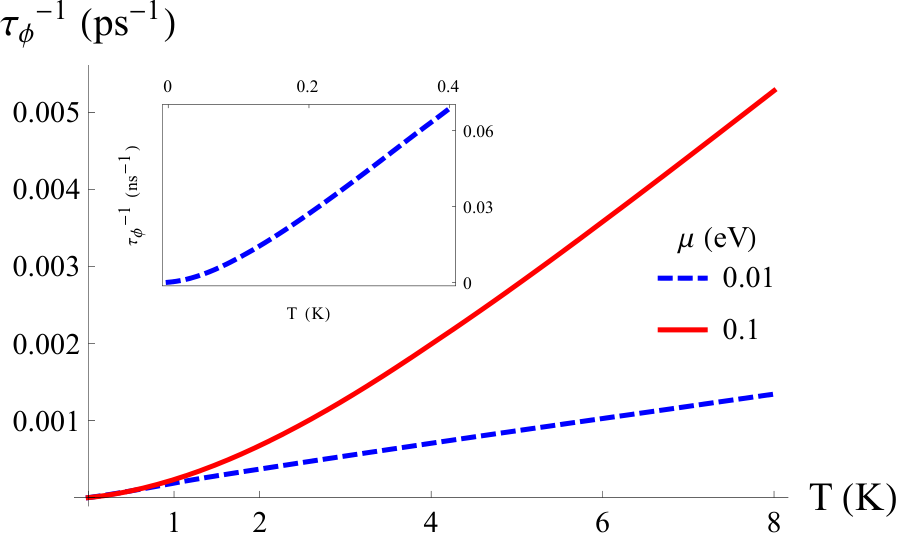
Note that besides the regions discussed in the main text, on the plane there exists another asymptotic region (IV), not mentioned in Eqs. (12m). It lies at very small densities below the blue line and above the line . In this region, the dephasing rate is still described by the GR, but contrary to region III, renormalization of the FP spectrum at low momenta is essential. In this situation, the dephasing rate equals . However, the relevant densities are so small, that this region does not fit into the scale of Fig. 3m.
It is instructive to compare the situation with flexural phonons to that for ordinary phonons in semiconductors, where the dephasing process can be viewed as coming from the energy diffusion via low-energy (i.e., quasi-elastic) collisions [4]. Under these conditions, the dephasing rate , where denotes the characteristic energy transfer during a single scattering event. Thus, the accumulation of phase in the course of the energy diffusion yields . The specific point of our problem, compared to dephasing via usual phonons, is that an electron is coupled to two flexural phonons, and dephasing cannot be described by the energy diffusion process. Because of this two-phonon interaction, the support of the correlation function of the fluctuations is not characterized by any typical frequency , and frequency transfer occurs in such a way that typical energy transfer is of the order of . In particular, this allows for an energy transfer exceeding , although the momentum transfer is limited by . As a result, the decay function at short times (i.e., in the non-GR regime) is proportional to , rather than as for the case of the energy diffusion. Note that the energy diffusion corresponds to the expansion of the factor which leads to the -dependence of . As we have already mentioned, in the case of FPs one cannot expand .
III.2 Vector potential coupling
III.2.1 Intervalley channel
The similarity (compare Eq. (24) with Eq. (26)) with the scalar potential case makes the calculation of asymptotes for the function straightforward. The function evolves with the growth of in the following fashion:
for
| (37) |
while for
| (38) |
Note that due to the absence of screening, dependence on is stronger than in the case of the scalar potential, compare Eq. (36) with Eq. (38).
Let us present some technical details. Here where and is defined in Eq. (31); specifically, for . In the GR region, the function is independent on . Its asymptotic behavior is given as follows:
Here, for (which is important for the convergence of the following integral),
| (41) |
and
| (42) |
where is the same as in the case of the scalar potential, and . For this yields and .
III.2.2 Intravalley channel
For the intravalley Cooperon, the function involves which does not vanish in the limit of . Therefore, it evolves with the growth of (i.e., from to ) as
| (43) |
where is defined in Eq. (III.2.1). It is noteworthy that the static deformations produce dephasing here. This happens because the electrons on the interfering trajectories are coupled to the vector potential of the same sign. The situation is similar to that for a particle in the random magnetic field [5, 6]. Unfortunately, the observation of this effect is obscured by the gaps inevitably produced in these channels by disorder scattering. The rate obtained from changes from to with increasing temperature, where
| (44) |
Here is the adiabatic parameter defined in the main text, and where describes the energy scale of the anharmonicity (see the main text). Note that for , the characteristic momentum transfer is instead of . As a result, the rate is independent of the chemical potential. Note also that for the intravalley channels the diffusive limit for the calculation of dephasing due to the el-FP interaction can be achieved at higher temperature as compared to the intervalley channels. For example, for dimensionless sheet conductance and chemical potential eV, the diffusive limit occurs already below K.
References
- [1] J. von Delft, F. Marquardt, R. A. Smith, and V. Ambegaokar, Phys. Rev. B 76, 195332 (2007).
- [2] E. McCann, K. Kechedzhi, V. I. Fal’ko, H. Suzuura, T. Ando, and B. L. Altshuler, Phys. Rev. Lett. 97, 146805 (2006).
- [3] F. Marquardt, J. von Delft, R. A. Smith, and V. Ambegaokar, Phys. Rev. B 76, 195331 (2007).
- [4] B. L. Altshuler, A. G. Aronov, and D. E. Khmelnitsky, Solid State Communications 39, 619 (1981).
- [5] A. G. Aronov, A. D. Mirlin, and P. Wölfle, Physical Review B 49, 16609 (1994).
- [6] A. G. Aronov and P. Wölfle, Phys. Rev. B 50, 16574 (1994).