Two Loop Neutrino Model with Dark Matter and Leptogenesis
Abstract
We study a two-loop induced radiative neutrino model at TeV scale with global symmetry, in which we analyze dark matter and resonant leptogenesis. The model includes two kinds of dark matter candidates. We discuss what kind of dark matter can satisfy the observed relic density as well as the current direct detection bound, and be simultaneously compatible with the leptogenesis. We also discuss whether our resonant leptogenesis can be differentiated from the other scenarios at TeV scale or not.
Keywords:
Radiative seesaw, Global symmetry, Dark matter, Resonant leptogenesisI Introduction
After the discovery of the Higgs boson at the LHC, the Standard Model (SM) has been established well. However the SM still has to be extended in order to explain the existence of dark matter (DM), the small neutrino masses, the baryon asymmetry in the universe and so on. Radiative seesaw scenarios are renowned as one of the economical models which simultaneously explain the existence of DM and the neutrino masses. Since the DM candidate is necessary to generate the neutrino masses in this kind of models, physics between DM and neutrinos is strongly correlated in this simple framework. For example, couplings and mass scale of DM are related with the neutrino mass scale. In addition, since this kind of models can naturally include a new particle with TeV scale mass, radiative seesaw scenarios have good testability in near future experiments. Along this line of idea, a vast literature has recently arisen in Ref. [1, 2, 3, 4, 5, 6, 7, 8, 9, 10, 11, 12, 13, 14, 15, 16, 17, 18, 19, 20, 21, 22, 23, 24, 25, 26, 27, 28, 29, 30, 31, 32, 33, 34, 35, 36, 37, 38, 39, 40, 41, 42, 43, 44, 45, 46, 47, 48, 49, 50, 51, 52, 53, 54, 55, 56, 57, 58, 59, 60, 61, 72, 62, 63, 64, 65, 66, 67, 68, 69, 70, 71].
On the other hand, explaining the observed baryon asymmetry in the universe via leptogenesis is one of the challenging issues in the framework of radiative seesaw models with right-handed neutrinos, since couplings related to the source of the leptogenesis are expected to be (1) due to the requirement of the neutrino masses. It causes the strong washout of the generated baryon asymmetry. In order to avoid this problem, we have to take hierarchical couplings with highly degenerated masses between the source and the mediated fields.11 1 Such couplings can be achieved by making use of the experimental fact that one of three neutrino masses can be negligible. To get the sufficient baryon asymmetry via thermal leptogenesis in the radiative seesaw framework, resonant leptogenesis would be only the solution that requires the mass degeneracy between the source and the mediated fields. For example, generating the baryon asymmetry via resonant leptogenesis has been discussed based on the Ma model [73].
In this paper, we study a two-loop induced radiative neutrino model at TeV scale with a global symmetry, in which we analyze DM and resonant leptogenesis simultaneously. In this model, we have a scalar or a fermion DM candidate. We discuss which kind of DM candidate can satisfy the observed relic density as well as the current direct detection bound, and can also be compatible with leptogenesis. Since our model has two sources of leptogenesis, we also show different points of our resonant leptogenesis from the other scenarios such as the Ma model at TeV scale [73].
This paper is organized as follows. In Sec. II, we show our model including field contents and their global charges, Higgs potential, and neutrino masses. In Sec. III, DM properties including relic density and current limit by direct detection experiments are discussed. In Sec. IV, we analyze resonant leptogenesis. Summary and conclusions are given in Sec. V.
II The Model
II.1 Model setup
| Accidental |
As shown in Tab. 1, we introduce two (or three) gauge singlet vector-like fermions , and gauge singlet Majorana fermions , and as new fermions. The number of these particles should be more than two in order to obtain at least two non-zero neutrino mass eigenvalues. We also introduce an inert doublet scalar , two neutral inert singlet scalars (), and a neutral singlet scalar as new scalars. We assume that only the Higgs doublet field in the SM and the new singlet scalar have vacuum expectation values (VEVs), which are symbolized by and respectively.22 2 The scale of should be larger than for successful leptogenesis as we will see later. Otherwise the annihilation channel whose reaction rate is determined by does not satisfy the out-of-equilibrium condition at where is the temperature of the universe. Thus the baryon asymmetry would be washed out due to this process. We impose a global symmetry, under which does not have a charge in order not to couple to the Goldstone boson (GB) [37]. The global charge is in principle an arbitrary, and the field assignments play a crucial role in realizing our neutrino masses at two-loop level. If the charge is fixed to be , we can identify this symmetry as a global symmetry. Hereafter we assume this global symmetry to be a kind of symmetry. Note that while the new fermions are added as vector-like and do not contribute to anomalies, this model is anomalous since the three chiral fermions with corresponding to the right-handed neutrinos are not introduced. If one would like to have an anomaly free model, the anomalies can be cancelled by introducing some pairs of new heavy vector-like fermions [74, 75]. However this is beyond the scope of this paper. This model has an accidental symmetry which can assure the DM stability, and the accidental assignments are shown in Tab. 1.
The renormalizable Lagrangian for Yukawa sector, mass term, and scalar potential under the charge assignments are given by
| (II.1) | |||||
| (II.2) | |||||
where the first term in generates the SM charged lepton masses, and we assume the couplings , , and in the scalar potential to be real for simplicity. As we will see below, these couplings become important for neutrino mass generation.
After the symmetry breaking, the scalar fields can be parametrized by
where GeV is the VEV of the SM Higgs doublet, and and are respectively the GBs which are absorbed by the longitudinal components of the and bosons. Inserting the tadpole conditions, the resulting mass matrix of the CP even scalar is given by
| (II.7) |
where is the SM-like Higgs boson and is an additional CP-even Higgs mass eigenstate. The gauge eigenstates and are rewritten in terms of the mass eigenstates and as
| (II.8) |
The GB in Eq. (II.1) appears due to the spontaneous symmetry breaking of the global symmetry. The couplings between the GB and the particles with non-trivial global charges are given by through the global current . As one can see, the coupling is suppressed by the VEV .
The mass matrices of the CP even and CP odd states of the inert scalar bosons are respectively given by
where we define diagonal mass matrices , and their mixing matrices , so that they satisfy . Depending on the couplings, the lightest CP even or CP odd mass eigenstate with the mass or can be a DM candidate.33 3 As we will discuss later, the CP even state is identified as DM. The non-standard couplings between DM and the GB induced by the non-self-conjugate couplings , , and may be relevant to compute the DM relic density. This coupling can be written down as
| (II.15) |
with the mixing matrix . In addition, the couplings between the CP even Higgs bosons and the GB are also relevant to compute the DM relic density. These couplings come from the kinetic term of and can be written as
| (II.16) |
Finally the mass eigenvalue of the charged inert scalar is given by
| (II.17) |
In this model, the typical mass scale of these new exotic particles is assumed to be TeV scale. On the other hand, we should take for successful leptogenesis. Therefore a certain degree of tuning among the relevant couplings cannot be avoided. More specifically, demanding that the diagonal elements of the mass matrix Eq. (II.7), (II.1) and (II.1) are TeV scale and off-diagonal elements are scale to obtain small mixings of the order of , the order of magnitude of the couplings should roughly be , , and , , , . Although this point may be a disadvantage of this model, it would be worth discussing such a new concrete model with a global symmetry as an example model since all the phenomenology of the neutrino masses, the existence of DM and the baryon asymmetry of the universe are closely correlated.
II.2 Neutrino mass matrix
Due to renormalizability and the strong restriction of interactions via the global symmetry in this model, neutrino masses are not generated neither tree level nor one-loop level. If the vector like fermion has a Majorana mass term, neutrino masses would be generated at one-loop level (for example see Ref. [1]), however this is not our case. As a result, neutrino masses are induced at two-loop level, and we have three types of diagrams as shown in Fig. 1. The formula of the total neutrino mass matrix can be given by
| (II.18) | |||||
where , a pair of and , a pair of and are the dimensionless loop functions which come from the left, center and right diagrams in Fig. 1 respectively. These loop functions are defined by
| (II.19) | |||||
| (II.20) | |||||
| (II.21) | |||||
| (II.22) | |||||
| (II.23) |
where and
| (II.24) | |||||
with . Note that in the derivation of the above formula, the CP phases except the Yukawa couplings are neglected.
The contribution of the left diagram can be understood as linear seesaw like formula by splitting the diagram into two Dirac masses induced at one-loop level. For the center and right diagrams, there are two kinds of contributions coming from right and left chiralities of the internal fermions. In other words, these two contributions to the neutrino masses come from the masses or momenta of the propagators in the loop respectively. The neutrino mass generation can be understood as follows. Due to the global symmetry breaking by the VEV of , the mixing between , and occurs. Then since the global symmetry is correlated with the lepton number conservation, the symmetry breaking implies breaking of the lepton number. Thus the neutrino Majorana mass term is generated after the symmetry breaking.
The neutrino mass matrix computed above can be diagonalized by the Pontecorvo-Maki-Nakagawa-Sakata matrix [76]; . The neutrino masses and their mixing angles are measured by experiments [77], and these values depend on normal or inverted mass hierarchy. In our model, the order of magnitude of the neutrino masses can roughly be estimated as where is the dominant Yukawa coupling in , , , , represents the mixing matrix of , , and is the loop function. Thus one can find that the order of is required to obtain the experimental value with the typical assumed mixing angle , and . Note that the neutrino mass matrix should be proportional to the VEV since is the origin of the lepton number violation.

We numerically compute the loop functions with the public code SecDec [78] in order to evaluate the neutrino masses more precisely in this model. Here one should note that the loop functions and include a divergence. This is obvious from the definition of the loop functions in Eq. (II.24) and (II.24). However the divergent terms eventually cancel out with each other as follows. The loop functions can be regularized with dimensional regularization and expanded around dimension which can be done within SecDec. With a brief evaluation, one can see that the terms including divergences are independent on at least either of or which is the index of the scalar mass eigenvalues. Thus the loop function including a divergence can be written as . Taking into account this fact and the orthogonality of the mixing matrices and which means , one can see that the first two terms and vanish after taking the summation over . Moreover the remaining third divergent term also cancels after all the relevant terms are summed in Eq. (II.22) and (II.23) as
| (II.29) | |||||
Thus the divergent terms do not contribute to the neutrino masses. The numerical value of the loop functions are almost fixed by the maximum mass in , , , and , and the result obtained by using SecDec is shown in Fig. 2.44 4 At most error is included in the numerical calculation. The numerical calculation shows that the loop function coming from the right diagram in Fig. 1 gives a dominant contribution to the neutrino masses.
II.3 LFV processes
We should take into account lepton flavor violations (LFVs) such as , which typically provide strong constraints on radiative neutrino mass models. In our case, such processes arise through only the term, and analyses are very similar with the case of the Ma model [79], and the Yukawa couplings , , , are not constrained by the LFV processes at least at one-loop level. Among the LFV processes, we focus on the one-loop induced that gives the most stringent constraint on and the mediating particles and . The resulting formula for and its experimental bound [80] are given by
| (II.30) | ||||
| (II.31) |
where GeV-2 is the Fermi constant, and is the electromagnetic fine structure constant. The simplest way to avoid this constraint is to assume to be diagonal, since its formula is proportional to the off-diagonal elements of as one can see in Eq. (II.30). In this case we expect the neutrino mixings can be derived through the other Yukawa couplings , , , . Otherwise the parameters are constrained as and . For instance, with the values , and , the maximum branching ratio is found to be .
Since we take for the LFV constraint and TeV of the new particle masses in the loop, the other Yukawa couplings , , , should be roughly larger than in order to obtain the scale of the observed neutrino mass eV assuming as discussed in the previous section.
II.4 Goldstone Boson
Here we mention some issues on the GB. Due to the direct consequence of our global symmetry, the GB remains as a physical state, which could be constrained by some experiments. In our case, the constraint comes from the invisible decay of the SM Higgs boson, and its decay width can be computed with the coupling given in Eq. (II.16) to be . This decay width should be smaller than 1.2 MeV at 95 confidential level [81], and thus we get the constraint
| (II.32) |
Moreover, itself is constrained by the latest LHC searches by ATLAS and CMS to be (conservatively) [82]. Therefore the above constraint is translated to the constraint on the VEV as . However since we take for successful leptogenesis, this bound is easily satisfied in our case.
Another bound comes from the Supernova 1987A observations and simulations, which tell us the following relation [83]:
| (II.33) |
This bound also does not affect to our model seriously, since both and are taken to be free values of physical parameters.
III Dark Matter

We have two DM candidates which are the lightest fermion and the lightest mass eigenstate of the scalars . These DM candidates can be stabilized by the accidental symmetry but not a remnant symmetry of the global symmetry. This accidental symmetry could be understood as a kind of the accidental symmetry which has been discussed for gauged in Ref. [84].
For the fermionic DM candidate , the relevant coupling for DM annihilations is only the Yukawa coupling , and the required strength of the Yukawa coupling is for the DM mass above the electroweak scale in order to accommodate the observed DM relic density. On the other hand, small coupling is needed to evade the LFV constraint as has been discussed in the previous section. Thus the fermionic DM candidate conflicts with the LFV constraint.55 5 Although the LFV constraint may be satisfied by considering a diagonal Yukawa matrix or specific flavor structure, we do not discuss this case.
Therefore we identify the lightest mass eigenstate of the scalars as a DM candidate. The mixing angles among are induced by the scalar couplings , , , and the magnitude of the mixing angles should roughly be in order to reproduce the measured neutrino masses without conflict with the process as discussed in the previous section. This order of the magnitude of the mixing angles can be achieved with the parameter setting given in Sec. II.1. Since the full scalar potential given by Eq. (II.2) is rather complicated, we take into account only , , , , , and for simplicity. Since the required order of the magnitude of the couplings , , , , is very small, they would not affect to the computation of the DM relic density and detection probability. However the coupling is important to induce the mixing angle , and is responsible for direct detection of DM since this coupling generates the dominant contribution to the elastic scattering with nuclei mediated by the SM-like Higgs boson .
The diagrams of the DM annihilations are shown in Fig. 3. The DM couplings in the scalar potential are basically weak in our parameter setting. However since the scalar DM candidate includes the doublet inert scalar , DM can annihilate into the gauge bosons via the gauge interactions in order to satisfy the observed DM relic density if the inert doublet scalar component of the DM candidate is sufficiently large. This can be achieved with a smaller compared to and in Eq. (II.1), and we consider such a case. In this case, the annihilation channels in the first line in Fig. 3 become dominant processes to determine the DM relic density.
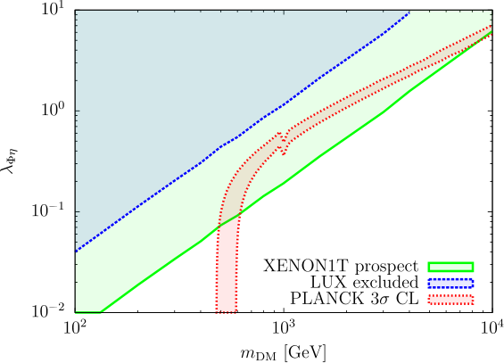
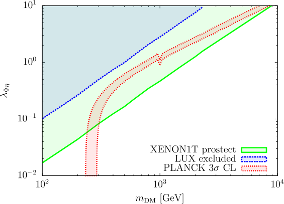
The DM relic density can be evaluated by using micrOMEGAs [85] and the results are shown in the (, ) plane in Fig. 4 where the heavier CP-even Higgs boson mass is taken to be and the mixing angle is as an example. Here we take the negative values of the scalar couplings , , . If the scalar couplings are positive, the lightest scalar in the imaginary components becomes DM candidate instead of the real components. The left plot shows the case that the masses of the other two heavier mass eigenstates are twice of the DM mass (lightest state), and the right plot shows the case that the heavier states are degenerate with the DM state. The red colored band represents the region satisfying the observed DM relic density by PLANCK within confidence level [86]. The blue region is excluded by the direct detection experiment LUX [87], and the green region is expected to be tested by the future direct detection experiment XENON1T [88]. From these plots, one can see that when the lightest DM state is non-degenerate with the other heavier states, DM is close to the inert doublet DM (left plot), because there is the mass threshold for the left plot in Fig. 4, which is the same property of the inert doublet DM [89]. As well-known, the inert doublet scalar DM candidate can satisfy the observed relic density in the mass ranges of and . On the other hand, the mass threshold can be lower as if and are degenerate with DM as one can see from the right plot in Fig. 4. This is because the interactions of the singlets and are described by the scalar potential, and extremely limited in the case of the simplified potential. There is a small resonance feature at due to the channel , however the resonance is not strong because of the small mixing angle .
IV Resonant leptogenesis
We consider the thermal leptogenesis in this model [90]. The lepton number asymmetry is expected to be generated through the out-of-equilibrium decay of the lightest Majorana fermions and , if we impose the lepton number of as . Although the Yukawa coupling is required to be smaller than from the LFV constraint, this is large enough that and the SM leptons are in the thermal equilibrium. Thus, the generated lepton number asymmetry in the sector can instantaneously be converted into the SM leptons, and then the baryon number asymmetry can be generated through sphaleron process.
After the global symmetry breaking, the Yukawa interactions for Majorana fermions are written as
| (IV.1) |
where and are expressed as the mass eigenstates of each Majorana fermion. Hereafter, we abbreviate them to and for convenience. The Yukawa couplings are redefined as
| (IV.2) |
where is the mixing angle of the -th generation.
.
In this model, we consider that the TeV scale masses of Majorana fermions and so that the annihilation channels are decoupled from the thermal bath before the temperature of the universe . Otherwise the generated lepton asymmetry would be washed out by these lepton number violating processes.
Although the TeV scale of the masses seems to be too small to realize the sufficient asymmetry associated with the decay processes for the generation of the required baryon number asymmetry, the generated baryon asymmetry can be enhanced by the resonance effect as known in resonant leptogenesis [91, 92, 93, 94, 95, 96, 97, 98, 99]. We define the parameter as the amplitude of the asymmetry. The dominant contribution for the asymmetry comes from the interference between the tree diagram and the one-loop self-energy diagram as depicted in the upper line in Fig. 5 and its formula is given by
| (IV.3) |
where and are the mass and the decay rate of respectively. From this equation, the maximum enhancement is caused when . In this model, we can take a larger compared to that of the second lightest right-handed neutrino in the canonical resonant leptogenesis at TeV scale, since the Yukawa couplings can be large without conflicting with the observed neutrino masses due to the loop suppression. Thus, the required magnitude of the degeneracy of the Majorana fermion mass can be quite milder to generate the sufficient baryon number asymmetry than those in the usual resonant leptogenesis at TeV scale [100, 73]. One may think that the baryon asymmetry should be correlated with the VEV of the singlet scalar since the breaking occurs with only . Indeed this breaking effect is included in the total mass matrix of , and the active neutrinos . For example, the violating Dirac mass term between and is induced at one-loop level as can be seen from the left diagram in Fig. 1. Thus the effect of the breaking is included in the masses of and , and one can understand that the baryon asymmetry is generated through the breaking effect in the mass matrix.
We need to take into account washout effects to evaluate the baryon number asymmetry. The generated lepton number asymmetry could be washed out through the lepton number violating 2-2 scattering processes and the inverse decay of . However, if the relevant Yukawa couplings are small enough, these processes can be nearly decoupled before the temperature of the thermal plasma decreases to . Thus, the washout of the generated lepton number asymmetry is expected to be suppressed sufficiently in this period. In order to examine this quantitatively, we numerically solve the coupled Boltzmann equations for the number density of and the lepton number asymmetry. We introduce the number density of , and the lepton number asymmetry in the comoving volume as , and respectively, by using the entropy density and the number densities which are expressed by , and . Their equilibrium values are given by , where is defined by , is the number of relativistic degrees of freedom and is the modified Bessel function of the second kind with the order . Since we assume is immediately translated into the SM leptons as we mentioned above, we use the relation which is derived from the chemical equilibrium condition in this model, and the baryon number asymmetry in the present Universe is estimated as , where is related to the sphaleron decoupling temperature .
The coupled Boltzmann equations for the leptogenesis in our model are written as [101]
| (IV.4) | |||
| (IV.5) | |||
| (IV.6) |
where is defined by
| (IV.7) |
with the modified Bessel function of the second kind with the order , is the reaction density for the scattering process which is given by
| (IV.8) |
with and the reduced cross section . There are two kinds of the processes and for the scattering processes as depicted in the bottom line of Fig. 5. The reduced cross section in our model is rather complicated since a lot of particles exist, but can be straightforwardly computed from the Lagrangian as same as Ref. [102, 103]. We solve the coupled Boltzmann equations numerically.
The decay of the lightest Majorana fermions should be out of thermal equilibrium so that the lepton number asymmetry can be generated through their decays. If we express the Hubble parameter as , this condition is given by at . Since we assume that each of the Majorana fermion mass is TeV, and TeV, the Yukawa couplings of and should be . On the other hand, the rest of the Yukawa couplings should be in order to generate the appropriate neutrino masses. Here we set Yukawa couplings in Eq. (IV.2) to be and and . We show the result for in Fig. 6 as an example, and also the generated baryon number asymmetry for each value of and in Fig. 7. Through this analysis, the masses of , and are fixed to be TeV and TeV respectively. These parameter set satisfies the condition for the DM phenomenology we discussed in the previous section.
From the left panel in Fig. 6, we can see that the required baryon number asymmetry can be obtained in this model. In the right panel, we plot the behavior of the relevant reaction rate for each process. This panel shows that the reaction rates of the inverse decay process and the lepton number-violating process induced by the s-channel exchange are quite large for a long time. Thus the baryon number asymmetry cannot be generated quickly until rather a late period. After , the generated baryon number asymmetry gradually increases and then the required value can be realized. This is because these processes are suppressed by the Boltzmann factor.
We show the relation between the generated baryon number asymmetry and the mass degeneracy of Majorana fermions in Fig. 7. Notice here that the generated baryon number asymmetry is always smaller than the required value in the case TeV. In this model, we can realize the large Yukawa couplings to explain the small neutrino mass due to the two-loop effects and then becomes larger compared to tree and one-loop neutrino mass models. Thus, the required mass degeneracy can be milder. However, the large Yukawa couplings cause the large washout effects. Since the Boltzmann suppression does not work well in the case of small , the large washout effects remain until quite a late period compared to the heavier cases. Thus the most of the generated baryon number asymmetry is washed out. We find that the observed baryon number asymmetry can be generated when the mass degeneracy is for TeV, as can be seen in Fig. 7. As we mentioned above, the magnitude of this mass degeneracy is quite milder than the canonical seesaw case for each value of due to the loop effects.66 6 The typical scale of is . It is also worth mentioning that the Ma model has an solution for [73].
V Conclusions
We have studied a two-loop induced radiative neutrino model at TeV scale with a global symmetry, in which two types of DM candidates (the lightest one of fermion or scalar) can be involved. The loop-induced neutrino masses have been evaluated appropriately and phenomenology of DM has also been discussed. The fermionic DM candidate is disfavored if we reproduce the measured neutrino masses and take into account the constraint from LFV with the same order of all the elements of . Then we have found that the scalar can be a good DM candidate which satisfies the observed relic density and the DM direct detection bound. We also found that the direct detection rate of DM is controlled by the coupling and some parameter region can be testable by the next future direct detection experiment XENON1T.
We have discussed baryon number asymmetry through the resonant leptogenesis with multi-sources scenario, in which the large Yukawa couplings (that is required to compensate the tiny neutrino masses at two-loop level) make the large asymmetry, but also cause the large washout effects. We have shown that the required baryon number asymmetry can be obtained for the parameter region i.e., for TeV, where or . In this case, the lightest Majorana fermions should satisfy TeV to suppress the washout effects by the Boltzmann factor. For larger , the required magnitude of the mass degeneracy is rather milder than the canonical seesaw case even at TeV scale models.
Acknowledgments
S. K. is supported by Grant-in-Aid for JSPS fellows (Grant No. 26 5862). H. O. expresses his sincere gratitude toward all the KIAS members, Korean cordial persons, foods, culture, weather, and all the other things. Y. O. is supported by the Korea Neutrino Research Center which is established by the National Research Foundation of Korea(NRF) grant funded by the Korea government(MSIP) (No. 2009-0083526). T. T. acknowledges support from P2IO Excellence Laboratory.
References
- [1] E. Ma, Phys. Rev. D 73, 077301 (2006) [hep-ph/0601225].
- [2] M. Aoki, J. Kubo and H. Takano, Phys. Rev. D 87, no. 11, 116001 (2013) [arXiv:1302.3936 [hep-ph]].
- [3] B. Dasgupta, E. Ma and K. Tsumura, Phys. Rev. D 89, no. 4, 041702 (2014) [arXiv:1308.4138 [hep-ph]].
- [4] L. M. Krauss, S. Nasri and M. Trodden, Phys. Rev. D 67, 085002 (2003) [arXiv:hep-ph/0210389].
- [5] M. Aoki, S. Kanemura and O. Seto, Phys. Rev. Lett. 102, 051805 (2009) [arXiv:0807.0361].
- [6] S. Baek, P. Ko, H. Okada and E. Senaha, JHEP 1409, 153 (2014) [arXiv:1209.1685 [hep-ph]].
- [7] D. Schmidt, T. Schwetz and T. Toma, Phys. Rev. D 85, 073009 (2012) [arXiv:1201.0906 [hep-ph]].
- [8] R. Bouchand and A. Merle, JHEP 1207, 084 (2012) [arXiv:1205.0008 [hep-ph]].
- [9] M. Aoki, J. Kubo, T. Okawa and H. Takano, Phys. Lett. B 707, 107 (2012) [arXiv:1110.5403 [hep-ph]].
- [10] Y. Farzan and E. Ma, Phys. Rev. D 86, 033007 (2012) [arXiv:1204.4890 [hep-ph]].
- [11] F. Bonnet, M. Hirsch, T. Ota and W. Winter, JHEP 1207, 153 (2012) [arXiv:1204.5862 [hep-ph]].
- [12] K. Kumericki, I. Picek and B. Radovcic, JHEP 1207, 039 (2012) [arXiv:1204.6597 [hep-ph]].
- [13] K. Kumericki, I. Picek and B. Radovcic, Phys. Rev. D 86, 013006 (2012) [arXiv:1204.6599 [hep-ph]].
- [14] E. Ma, Phys. Lett. B 717, 235 (2012) [arXiv:1206.1812 [hep-ph]].
- [15] G. Gil, P. Chankowski and M. Krawczyk, Phys. Lett. B 717, 396 (2012) [arXiv:1207.0084 [hep-ph]].
- [16] H. Okada and T. Toma, Phys. Rev. D 86, 033011 (2012) arXiv:1207.0864 [hep-ph].
- [17] D. Hehn and A. Ibarra, Phys. Lett. B 718, 988 (2013) [arXiv:1208.3162 [hep-ph]].
- [18] P. S. B. Dev and A. Pilaftsis, Phys. Rev. D 86, 113001 (2012) [arXiv:1209.4051 [hep-ph]].
- [19] Y. Kajiyama, H. Okada and T. Toma, Eur. Phys. J. C 73, no. 3, 2381 (2013) [arXiv:1210.2305 [hep-ph]].
- [20] H. Okada, arXiv:1212.0492 [hep-ph].
- [21] M. Aoki, S. Kanemura, T. Shindou and K. Yagyu, JHEP 1007, 084 (2010) [Erratum-ibid. 1011, 049 (2010)] [arXiv:1005.5159 [hep-ph]].
- [22] S. Kanemura, O. Seto and T. Shimomura, Phys. Rev. D 84, 016004 (2011) [arXiv:1101.5713 [hep-ph]].
- [23] M. Lindner, D. Schmidt and T. Schwetz, Phys. Lett. B 705, 324 (2011) [arXiv:1105.4626 [hep-ph]].
- [24] S. Kanemura, T. Nabeshima and H. Sugiyama, Phys. Rev. D 85, 033004 (2012) [arXiv:1111.0599 [hep-ph]].
- [25] S. Kanemura and H. Sugiyama, Phys. Rev. D 86, 073006 (2012) [arXiv:1202.5231 [hep-ph]].
- [26] P. -H. Gu and U. Sarkar, Phys. Rev. D 77, 105031 (2008) [arXiv:0712.2933 [hep-ph]].
- [27] P. -H. Gu and U. Sarkar, Phys. Rev. D 78, 073012 (2008) [arXiv:0807.0270 [hep-ph]].
- [28] M. Gustafsson, J. M. No and M. A. Rivera, Phys. Rev. Lett. 110, 211802 (2013) arXiv:1212.4806 [hep-ph].
- [29] Y. Kajiyama, H. Okada and K. Yagyu, Nucl. Phys. B 874, 198 (2013) [arXiv:1303.3463 [hep-ph]].
- [30] Y. Kajiyama, H. Okada and T. Toma, Phys. Rev. D 88, 015029 (2013) [arXiv:1303.7356].
- [31] A. E. Carcamo Hernandez, I. d. M. Varzielas, S. G. Kovalenko, H. Päs and I. Schmidt, Phys. Rev. D 88, 076014 (2013) [arXiv:1307.6499 [hep-ph]].
- [32] A. E. Carcamo Hernandez, RMartinez and F. Ochoa, arXiv:1309.6567 [hep-ph].
- [33] K. L. McDonald, JHEP 1311, 131 (2013) [arXiv:1310.0609 [hep-ph]].
- [34] H. Okada and K. Yagyu, Phys. Rev. D 89, no. 5, 053008 (2014) [arXiv:1311.4360 [hep-ph]].
- [35] S. Baek, H. Okada and T. Toma, JCAP 1406, 027 (2014) [arXiv:1312.3761 [hep-ph]].
- [36] E. Ma, Phys. Lett. B 732, 167 (2014) [arXiv:1401.3284 [hep-ph]].
- [37] S. Baek, H. Okada and T. Toma, Phys. Lett. B 732, 85 (2014) [arXiv:1401.6921 [hep-ph]].
- [38] A. Ahriche, S. Nasri and R. Soualah, Phys. Rev. D 89, no. 9, 095010 (2014) [arXiv:1403.5694 [hep-ph]].
- [39] S. Kanemura, T. Nabeshima and H. Sugiyama, Phys. Lett. B 703, 66 (2011) [arXiv:1106.2480 [hep-ph]].
- [40] S. Kanemura, T. Matsui and H. Sugiyama, Higgs Doublet Model,” Phys. Lett. B 727, 151 (2013) [arXiv:1305.4521 [hep-ph]].
- [41] H. Okada and K. Yagyu, Phys. Rev. D 90, no. 3, 035019 (2014) [arXiv:1405.2368 [hep-ph]].
- [42] S. Kanemura, T. Matsui and H. Sugiyama, Phys. Rev. D 90, 013001 (2014) [arXiv:1405.1935 [hep-ph]].
- [43] C. S. Chen, K. L. McDonald and S. Nasri, Phys. Lett. B 734, 388 (2014) [arXiv:1404.6033 [hep-ph]].
- [44] A. Ahriche, K. L. McDonald and S. Nasri, JHEP 1410, 167 (2014) [arXiv:1404.5917 [hep-ph]].
- [45] H. Okada, arXiv:1404.0280 [hep-ph].
- [46] A. Ahriche, C. S. Chen, K. L. McDonald and S. Nasri, Phys. Rev. D 90, 015024 (2014) [arXiv:1404.2696 [hep-ph]].
- [47] M. Aoki and T. Toma, JCAP 1409, 016 (2014) [arXiv:1405.5870 [hep-ph]].
- [48] M. Lindner, S. Schmidt and J. Smirnov, JHEP 1410, 177 (2014) [arXiv:1405.6204 [hep-ph]].
- [49] Y. H. Ahn and H. Okada, Phys. Rev. D 85, 073010 (2012) [arXiv:1201.4436 [hep-ph]].
- [50] E. Ma, A. Natale and A. Rashed, Int. J. Mod. Phys. A 27, 1250134 (2012) [arXiv:1206.1570 [hep-ph]].
- [51] Y. Kajiyama, H. Okada and K. Yagyu, JHEP 10, 196 (2013) arXiv:1307.0480 [hep-ph].
- [52] Y. Kajiyama, H. Okada and K. Yagyu, Nucl. Phys. B 887, 358 (2014) [arXiv:1309.6234 [hep-ph]].
- [53] E. Ma, Phys. Rev. Lett. 112, 091801 (2014) [arXiv:1311.3213 [hep-ph]].
- [54] E. Ma and A. Natale, Phys. Lett. B 734, 403 (2014) [arXiv:1403.6772 [hep-ph]].
- [55] S. Kanemura, M. Kikuchi and K. Yagyu, Nucl. Phys. B 896, 80 (2015) [arXiv:1502.07716 [hep-ph]].
- [56] S. Bahrami and M. Frank, Phys. Rev. D 91, 075003 (2015) [arXiv:1502.02680 [hep-ph]].
- [57] S. Baek, H. Okada and K. Yagyu, JHEP 1504, 049 (2015) [arXiv:1501.01530 [hep-ph]].
- [58] H. Hatanaka, K. Nishiwaki, H. Okada and Y. Orikasa, Nucl. Phys. B 894, 268 (2015) [arXiv:1412.8664 [hep-ph]].
- [59] H. Okada and Y. Orikasa, arXiv:1412.3616 [hep-ph].
- [60] D. Aristizabal Sierra, A. Degee, L. Dorame and M. Hirsch, JHEP 1503, 040 (2015) [arXiv:1411.7038 [hep-ph]].
- [61] H. Okada, T. Toma and K. Yagyu, Phys. Rev. D 90, no. 9, 095005 (2014) [arXiv:1408.0961 [hep-ph]].
- [62] A. E. Carcamo Hernandez and R. Martinez, arXiv:1501.05937 [hep-ph].
- [63] A. E. C. Hernandez and R. Martinez, arXiv:1501.07261 [hep-ph].
- [64] P. Culjak, K. Kumericki and I. Picek, Phys. Lett. B 744, 237 (2015) [arXiv:1502.07887 [hep-ph]].
- [65] P. Humbert, M. Lindner and J. Smirnov, JHEP 1506, 035 (2015) [arXiv:1503.03066 [hep-ph]].
- [66] H. Okada, arXiv:1503.04557 [hep-ph].
- [67] C. Q. Geng and L. H. Tsai, arXiv:1503.06987 [hep-ph].
- [68] H. Okada, N. Okada and Y. Orikasa, arXiv:1504.01204 [hep-ph].
- [69] C. Q. Geng, D. Huang and L. H. Tsai, Phys. Lett. B 745, 56 (2015) [arXiv:1504.05468 [hep-ph]].
- [70] A. Ahriche, K. L. McDonald, S. Nasri and T. Toma, Phys. Lett. B 746, 430 (2015) [arXiv:1504.05755 [hep-ph]].
- [71] A. Ahriche, K. L. McDonald and S. Nasri, arXiv:1504.06759 [hep-ph].
- [72] Hiroshi Okada, Yuta Orikasa, Phys.Rev. D90, 075023 (2014), arXiv:1407.2543 [hep-ph].
- [73] S. Kashiwase and D. Suematsu, Eur. Phys. J. C 73, 2484 (2013) [arXiv:1301.2087 [hep-ph]].
- [74] T. Appelquist, B. A. Dobrescu and A. R. Hopper, Phys. Rev. D 68, 035012 (2003) [hep-ph/0212073].
- [75] P. Batra, B. A. Dobrescu and D. Spivak, J. Math. Phys. 47, 082301 (2006) [hep-ph/0510181].
- [76] Z. Maki, M. Nakagawa and S. Sakata, Prog. Theor. Phys. 28, 870 (1962).
- [77] D. V. Forero, M. Tortola and J. W. F. Valle, Phys. Rev. D 90, no. 9, 093006 (2014) [arXiv:1405.7540 [hep-ph]].
- [78] S. Borowka, G. Heinrich, S. P. Jones, M. Kerner, J. Schlenk and T. Zirke, Comput. Phys. Commun. 196, 470 (2015) [arXiv:1502.06595 [hep-ph]].
- [79] T. Toma and A. Vicente, JHEP 1401, 160 (2014) [arXiv:1312.2840 [hep-ph]].
- [80] J. Adam et al. [MEG Collaboration], Phys. Rev. Lett. 110, 201801 (2013) [arXiv:1303.0754 [hep-ex]].
- [81] K. Cheung, J. S. Lee and P. Y. Tseng, JHEP 1305, 134 (2013) [arXiv:1302.3794 [hep-ph]].
- [82] T. Robens and T. Stefaniak, Eur. Phys. J. C 75, no. 3, 104 (2015) [arXiv:1501.02234 [hep-ph]].
- [83] W. Y. Keung, K. W. Ng, H. Tu and T. C. Yuan, Phys. Rev. D 90, no. 7, 075014 (2014) doi:10.1103/PhysRevD.90.075014 [arXiv:1312.3488 [hep-ph]].
- [84] M. Ibe, S. Matsumoto and T. T. Yanagida, Phys. Lett. B 708, 112 (2012) [arXiv:1110.5452 [hep-ph]].
- [85] G. Belanger, F. Boudjema, A. Pukhov and A. Semenov, Comput. Phys. Commun. 185, 960 (2014) [arXiv:1305.0237 [hep-ph]].
- [86] P. A. R. Ade et al. [Planck Collaboration], arXiv:1502.01589 [astro-ph.CO].
- [87] D. S. Akerib et al. [LUX Collaboration], Phys. Rev. Lett. 112, 091303 (2014) [arXiv:1310.8214 [astro-ph.CO]].
- [88] E. Aprile [XENON1T Collaboration], Springer Proc. Phys. 148, 93 (2013) [arXiv:1206.6288 [astro-ph.IM]].
- [89] T. Hambye, F.-S. Ling, L. Lopez Honorez and J. Rocher, JHEP 0907, 090 (2009) Erratum: [JHEP 1005, 066 (2010)] [arXiv:0903.4010 [hep-ph]].
- [90] M. Fukugita and T. Yanagida, Phys. Lett. B 174, 45 (1986).
- [91] M. Flanz, E. A. Paschos and U. Sarkar, Phys. Lett. B 345, 248 (1995) [Erratum-ibid. B 382, 447 (1996)] [hep-ph/9411366].
- [92] L. Covi, E. Roulet and F. Vissani, Phys. Lett. B 384, 169 (1996) [hep-ph/9605319].
- [93] A. Pilaftsis, Phys. Rev. D 56, 5431 (1997) [hep-ph/9707235].
- [94] E. K. Akhmedov, M. Frigerio and A. Y. Smirnov, JHEP 0309, 021 (2003) [hep-ph/0305322].
- [95] C. H. Albright and S. M. Barr, Phys. Rev. D 69, 073010 (2004) [hep-ph/0312224].
- [96] T. Hambye, J. March-Russell and S. M. West, JHEP 0407, 070 (2004) [hep-ph/0403183].
- [97] A. Pilaftsis and T. E. J. Underwood, Nucl. Phys. B 692, 303 (2004) [hep-ph/0309342].
- [98] A. Pilaftsis and T. E. J. Underwood, Phys. Rev. D 72, 113001 (2005) [hep-ph/0506107].
- [99] P. S. Bhupal Dev, P. Millington, A. Pilaftsis and D. Teresi, Nucl. Phys. B 886, 569 (2014) [arXiv:1404.1003 [hep-ph]].
- [100] S. Kashiwase and D. Suematsu, Phys. Rev. D 86, 053001 (2012) [arXiv:1207.2594 [hep-ph]].
- [101] E. W. Kolb and S. Wolfram, Nucl. Phys. B 172, 224 (1980) [Erratum-ibid. B 195, 542 (1982)].
- [102] M. A. Luty, Phys. Rev. D 45, 455 (1992).
- [103] M. Plumacher, Nucl. Phys. B 530, 207 (1998) [hep-ph/9704231].