Graph Partitioning via Parallel Submodular Approximation
to Accelerate Distributed Machine Learning
Abstract
Distributed computing excels at processing large scale data, but the communication cost for synchronizing the shared parameters may slow down the overall performance. Fortunately, the interactions between parameter and data in many problems are sparse, which admits efficient partition in order to reduce the communication overhead.
In this paper, we formulate data placement as a graph partitioning problem. We propose a distributed partitioning algorithm. We give both theoretical guarantees and a highly efficient implementation. We also provide a highly efficient implementation of the algorithm and demonstrate its promising results on both text datasets and social networks. We show that the proposed algorithm leads to 1.6x speedup of a state-of-the-start distributed machine learning system by eliminating 90% of the network communication.
1 Introduction
The importance of large-scale machine learning continues to grow in concert with the big data boom, the advances in learning techniques, and the deployment of systems that enable wider applications. As the amount of data scales up, the need to harness increasingly large clusters of machines significantly increases. In this paper, we address a question that is fundamental for applying today’s loosely-coupled “scale-out” cluster computing techniques to important classes of machine learning applications:
How to spread data and model parameters across a cluster of machines for efficient processing?
One big challenge for large-scale data processing problems is to distribute the data over processing nodes to fit the computation and storage capacity of each node. For instance, for very large scale graph factorization [2], one needs to partition a natural graph in a way such that the memory, which is required for storing local state of the partition and caching the adjacent variables, is bounded within the capacity of each machine. Similar constraints apply to GraphLab [20, 12], where vertex-specific updates are carried out while keeping other variables synchronized between machines. Likewise, in distributed inference for graphical models with latent variables [1, 26], the distributed state variables must be synchronized efficiently between machines. Furthermore, general purposed distributed machine learning framework such as the parameter server [18, 8] face similar issues when it comes to data and parameter layout.
Shared parameters are synchronized via the communication network. The sheer number of parameters and the iterative nature of machine learning algorithms often produce huge amounts of network traffic. Figure 1 shows that, if we randomly assign data (documents) to machines in a text classification application, the total amount of network traffic is 100 times larger than the size of training data. Specifically, almost 4 TB parameters are communicated for 300 GB training data. Given that the network bandwidth is typically much smaller than the local memory bandwidth, this traffic volume can potentially become a performance bottleneck.
There are three key challenges in achieving scalability for large-scale data processing problems:
- Limited computation (CPU) per machine:
-
therefore we need a well-balanced task distribution over machines.
- Limited memory (RAM) per machine:
-
the amount of storage per machine available for processing and caching model variables is often constrained to a small fraction of the total model.
- Limited network bandwidth:
-
the network bandwidth is typically 100 times worse than the local memory bandwidth. Thus we need to reduce the amount of communication between machines.
One key observation is the sparsity pattern in large scale datasets: most documents contain only a small fraction of distinct words, and most people have only a few friends in a social graph. Such nonuniformity and sparsity is both a boon and a challenge for the problem of dataset partitioning. Due to its practical importance, even though the dataset partitioning problems are often NP hard [28], it is still worth seeking practical solutions that outperform random partitioning, which typically leads to poor performance.
Our contributions: In this paper, we formulate the task of data and parameter placement as a graph partitioning problem. We propose Parsa , a PARallel Submodular Approximation algorithm for solving this problem, and we analyze its theoretical guarantees. A straightforward implementation of the algorithm has running time in the order of , where is the number of partitions and is the number of edges in the graph. Using an efficient vertex selection data structure, we provide an efficient implementation with time complexity . We also discuss the techniques including sampling, initialization and parallelization to improve the partitioning quality and efficiency.
Experiments on text datasets and social networks of various scales show that, on both partition quality and time efficiency, Parsa outperforms state-of-the-art methods, including METIS [16], PaToH [6] and Zoltan [9]. Parsa can also significantly accelerate the parameter server, a state-of-the-art general purpose distributed machine learning, on data of hundreds GBs size and with billions parameters.
2 Graph Partitioning
In this section, we first introduce the inference problem and the model of dependencies in distributed inference. Then we provide the formulation of the data partitioning problem in distributed inference. We also present a brief overview of related work in the end.
2.1 Inference in Machine Learning
In machine learning, many inference problems have graph-structured dependencies. For instance, in risk minimization [14], we strive to solve
| (1) |
where is a loss function measuring the model fitting error in the data , and is a regularizer on the model parameter . The data and parameters are often correlated only via the nonzero terms in , which exhibit sparsity patterns in many applications. For example, in email spam filtering, elements of ’ correspond to words and attributes in emails, while in computational advertising, they correspond to words in ads and user behavior patterns.
For undirected graphical models [4, 17], the joint distribution of the random variables in logscale can be written as a summation of potential of all the cliques in the graph, and each clique potential only depends on the subset of variables in the clique .
The learning and inference problems in undirected graphical models are often formulated as an optimization problem in the following form:
| (2) |
where local variables interact through the model parameters of the cliques.
Similar problems occur in the context of inference on natural graphs [3, 12, 2], where we have sets of interacting parameters represented by vertices on the graph, and manipulating a vertex affects all of its neighbors computationally.

2.2 Bipartite Graphs
The dependencies in the inference problems above can be modeled by a bipartite graph with vertex sets and and edge set . We denote the edge between two node and by . Figure 2 illustrates the case of risk minimization (1), where consists of the samples and consists of the parameters in . There is an edge if and only if the -th element of is non-zero. Therefore, is the working set of elements of for evaluating the loss function on the sample .
We can construct such bipartite graph to encode the dependencies in undirected graphical models and natural graphs with node set and edge set . One construction is to define , and add an edge to the edge set if they are connected in the original graph. An alternative construction is to define the node set to be , the set of all cliques of the original graph, and add an edge to the edge set if node belongs to the clique in the original graph.
Throughout the discussion, we refer to as the set of data (examples) nodes and as the set of parameters (results) nodes.

2.3 Distributed Inference
The challenge for large scale inference is that the size of the optimization problem in (2) is too large, and even the model may be too large to be stored on a single machine. One solution is to divide exploit the additive form of to decompose the optimization into smaller problems, and then employ multiple machines to solve these sub-problems while keeping the solutions (parameters) consistent.
There exist several frameworks to simplify the developing of efficient distributed algorithms, such as Hadoop [11] and its in-memory variant Spark [34] to execute MapReduce programs, and Graphlab for distributed graph computation [21]. In this paper, we focus on the parameter server framework [18], a high-performance general-purpose distributed machine learning framework.
In the parameter server framework, computational nodes are divided into server nodes and worker nodes, which are shown in Figure 3. The globally shared parameters are partitioned and stored in the server nodes. Each worker node solves a sub-problem and communicates with the server nodes in two ways: to push local results such as gradients or parameter updates to the servers, and to pull recent parameter (changes) from the servers. Both push and pull are executed asynchronously.
2.4 Multiple Objectives of Partitioning

In distributed inference, we divide the problem in (2) by partition the cost function as well as the associated dependency graph into blocks. Without loss of generality we consider a parameter server with server nodes and worker nodes, and each machine has exactly one server and one worker (otherwise we can aggregate multiple nodes in the same machines without affecting the following analysis). For the bipartite dependency graph , we partition the parameter set into parts and assign each part to a server node, and we partition the data set into parts and assign them to individual worker nodes. Figure 4 illustrates an example for . More specifically, we want to divide both and into non-overlapping parts
| (3) |
and assign the part and to the worker node and server node on machine respectively.
There are three goals when implementing the graph partitioning:
Balancing the computational load. We want to ensure that each machine has approximately the same computational load. Assume that each example incurs roughly the same workload, then one of the objective to keep small:
| (4) |
Satisfying the memory constraint. Inference algorithms frequently access the parameters (at random). Workers keep these parameters in memory to improve performance, yet RAM is limited. Denote by the neighbor set of
| (5) |
Then is the working set of the parameters worker needed. For simplicity we assume that each parameter has the same storage cost. Our goal to limit the worker’s memory footprint is given by
| (6) |
Minimizing the communication cost. The total communication cost per worker is , which is already minimized using our previous goal (6). To further reduce this cost, we can assign server to the same machine with worker , so that any communication uses memory rather than network. This reduces the inter-machine communication cost to . Figure 4 shows an example. Further note that if is not needed by worker , then server should never maintain . In other words, we have and the cost simplifies to .
On the other hand, is the communication cost of server because other workers must request parameters from server . Therefore, the goal to minimize the maximal communication cost of a machine is
| (7) |
2.5 Related Work
Graph partitioning has attracted much interest in scientific computing [16, 6, 9], scaling out large-scale computations [12, 35, 33, 5, 13, 31], graph databases [25, 32, 7], search and social network analysis [24, 31, 2], and streaming processing [28, 27, 22, 30].
Most previous work, such as METIS [16], is concerned with edge cuts. Only a few of them solve the vertex cut problem, which is closely related to this paper, to directly minimize the network traffic. PaToH [6] and Zoltan [9] used multilevel partitioning algorithms related to METIS, while PowerGraph [12] adopted a greedy algorithm. Very recently [5] studied the relation between edge cut and vertex cut.
Different to these works, we propose a new algorithm based on submodular approximation to solve the vertex-cut partitioning problem. We give theoretical analysis of the partition quality, and describe an efficient distributed implementation. We show that the proposed algorithm outperforms the state of the art on several large scale real datasets in both in terms of quality and speed.
3 Algorithm
In this section, we present our algorithm Parsa for solving the partitioning problem with multiple objectives in (4), (6) and (7).
Note that (6) is equal to a -way graph partition problem on vertex set with vertex-cut as the merit. This problem is NP-Complete [6]. Furthermore, (7) is more complex because of the involvement of . Rather than solving all these objectives together, Parsa decomposes this problem into two tasks: partition the data by solving (4) and (6), and given the partition of partition the parameters by solving (7). Intuitively, we first assigns data workers to balance the CPU load and minimize the memory footprint, and then distribute the parameters over servers to minimize inter-machine communication.
3.1 Partitioning over Worker Nodes
Note that is a set function in the variable . It is a submodular function similar to convex and concave functions in real variables. Although the problem in (4) is NP-Complete, there exist several algorithms to solve it approximately by exploiting the submodularity [29]. In our algorithm, we modified [29] to solve (4) and (6). The key difference is that we build up the sets incrementally, which is important for both partition quality and computational efficiency at a later stage.
As shown in Algorithm 1, the algorithm proceeds as follows: in each round we pick the smallest partition and find the best set of elements to add to it. To do so, we first draw a small subset of candidates and select the best subset using a minimum-increment weight via . If the optimal solution satisfies , i.e., the cost for increasing is not too large, we assign to partition .
Before showing the implementation details in Section 4, we first analyze the partitioning quality of Algorithm 1.
Proposition 1
Assume that there exists some partitioning that satisfies . Let , , and . Then Algorithm 1 will succeed with probability at least and it will generate a feasible solution with partitioning cost at most .
Proof.
The proof is near-identical as [29]. Note that we overload the meaning of as it refers to the remaining variables in the algorithm.
For a given iteration, without loss of generality we assume that maximizes for all . Denote this by . Since is the optimal solution at the current iteration we have . Further note that by monotonicity and submodularity . Moreover, holds since contains only the leftovers. Consequently . Finally, the algorithm only increases the size of whenever the cost is balanced. Hence . Combining this yields
Using the results from the proof of [29, Theorem 5.4] we know that and therefore happens with probability at least . Hence the probability of removing at least one vertex from within an iteration is greater than .
Chernoff bounds show that after iterations the algorithm will terminate with probability at least since the residual is small, i.e., .
The algorithm will never select a for augmentation unless (there would always be a smaller set). Moreover, the maximum increment at any given time is . Hence and therefore .
Finally, the contribution of the unassigned residual is at most since each is incremented by at most elements and since for all . In summary, this yields . ∎
3.2 Partitioning over Server Nodes
Next, given the partition of , we find an assignment of parameters in to servers. We reformulate (7) as a convex integer programming problem with totally unimodular constraints [15], which is then solved using a sequential optimization algorithm performing a sweep through the variables.
We define index variables , to indicate which server node maintains a particular parameter . They need to satisfy . Moreover, denote by variables that record whether . Then we can rewrite (7) as a convex integer program:
| (8a) | ||||
| subject to | (8b) | |||
Here we exploited the fact that and that . These constraints are totally unimodular, since they satisfy the conditions of [15]. As a consequence every vertex solution is integral and we may relax the condition to to obtain a convex optimization problem.
Algorithm 2 performs a single sweep over (8) to find a locally optimal assignment of one variable at a time. We found that it is sufficient for a near-optimal solution. Repeated sweeps over the assignment space are straightforward and will improve the objective until convergence to optimality in a finite number of steps: due to convexity all local optima are global. Further note that we need not store the full neighbor sets in memory. Instead, we can perform the assignment in a streaming fashion.
4 Efficient Implementation
The time complexity of Algorithm 2 is , however, it could be for Algorithm 1, which is infeasible in practice. We now discuss how to implement Algorithm 1 efficiently. We first present how to find the optimal and sample . Then we address the parallel implementation with the parameter server, and finally describe neighbor set initialization to improve the partition quality.
4.1 Finding efficiently
The most expensive operation in the inner loop of Algorithm 1 is step 10, determining which vertices, , to add to a partition. Submodular minimization problems incur time [23]. Given the fact that this step is invoked frequently and the problem is large, this strategy is impractical. A key approximation Parsa made is to add only a single vertex at a time instead of a set of vertices: Given a vertex set and partition , it finds vertex that minimizes
| (9) |
An additional advantage of this approximation is that we are now solving exactly the CPU load balancing problem (4). Since we only assign one vertex at a time to the smallest partition, we obtain perfect balancing.
Even though this approximation improves the performance, a naive way to calculate (9) is to compute all to find with the minimal value for each iteration. If the size of is a constant fraction of the entire graph, this leads to an undesirable time complexity of . This remains impractical for graphs with billions of vertices and edges.
We accelerate computation as follows: we store all vertex costs to avoid re-computing them, and we create a data structure to locate the lowest-cost vertex efficiently.
Storing vertex costs. If we subtract the constant from , we obtain the vertex cost
| (10) |
This is the number of new vertices that would be added to the neighbor set of partition due top adding vertex to .
When adding to a partition , only the costs of a few vertices will be changed. Denote by
the set of new vertices will be added into the neighbor set of when assigning to partition . Only vertices in connected to vertices in will have their costs affected, and these costs will only be reduced and never increased. Due to the sparsity of the graph, this is often a small subset of the total vertices. Hence the overhead of updating the vertex costs is much smaller than re-computing them repeatedly.
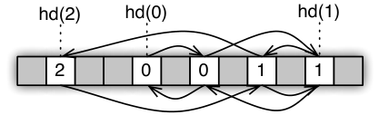
Fast vertex cost lookup. We build an efficient data structure to store the vertex costs, which is illustrated at Figure 5. For each partition , we use an array to store the -th vertex cost, , in the -th entry, denoted by . We then impose a doubly-linked list on top of this array in an increasing order to rapidly locate the lowest-cost vertex. When a vertex cost is modified (always reduced), we update the doubly-linked list to preserve the order.
Note that most large-scale graphs have a power-law degree distribution. Therefore a large portion of vertex costs will be small integers, which are always less equal that their degrees. We store a small array of “head” pointers to the locations in the list where the cost jumps to . The pointers accelerate locating elements in the list when updating. In practice, we found covers over 99% of vertex costs.
The algorithm is illustrated in Algorithm 3. The inputs are a bipartite graph , the number of partitions , together with sets , which is the union neighbor set of vertices have been assigned to partition before. The outputs are the partitions and updated with the neighbor set of included. Here we assume , the sampling strategy of will be addressed in next section.
Runtime. The initial can be computed in time and then be ordered in by counting sort, as they are integers, upper bounded by the maximal vertex degree. The most expensive part of Algorithm 3 is updating in step 13. This is are evaluated at most times because, for each partition, a vertex together with its neighbors is accessed at most once.
For most cases, the time complexity of updating the doubly-linked lists is . The cost to access the -th vertex is due to the sequential storing on an array. Finding a vertex with the minimal value or removing a vertex from the list is also in time because of the doubly links. Keeping the list ordered after decreasing a vertex cost by is in most cases ( for the worst case), as discussed above, by using the cached head pointers.
4.2 Division into Subgraphs
One goal of the sampling strategy used in Algorithm 1 is to keep the partitions of balanced, because the vertices assigned to a partition at a time is being limited. The additional constraint introduced in the previous section ensures that only a single vertex is assigned each time, which addresses balancing. Consequently we would like to sample as many vertices as possible to enlarge the search range of the optimal to partition quality. Sampling remains appealing since it is a trade-off between computation efficiency and partition quality.
Parsa first randomly divides into blocks. It next constructs the corresponding subgraphs by adding the neighbor vertices from and the corresponding edges, and then partitions these subgraphs sequentially by Algorithm 3. In other words, denote by the subgraphs, and the initialized neighbor sets, for instances for all ; at iteration , we sequentially feed and ’s into Algorithm 3 to obtain the partitions of and updated ’s, which contain the previous partition information. Then we union the results on each subgraph to the final partitions of by for .
Compared to the scheme described in Section 3.1 which samples a new subgraph () for each single vertex assignment, Parsa fixes those subgraphs at the beginning. This sampling strategy has several advantages. First, it partitions a subgraph by directly using Algorithm 3, which takes advantage of the head pointers and linked list to improve the efficiency. Next, it is convenient to place both the initialization of neighbor sets and parallelization which will be introduced soon on subgraph granularity. Finally, this strategy is I/O efficient, because we must only keep the current subgraph in memory. As a result, it is possible to partition graphs of sizes much larger than physical memory.
The number of subgraphs is a trade-off between partition quality and computational efficiency. In the extreme case of , the vertex assigned to a partition is the optimal one from all unassigned vertices. It is, however, the most time consuming. In contrast, though the time complexity reduces to when letting , we only get random partition results. Therefore, a well-chosen size not only removes the graph size constraint but also balances time and quality.
4.3 Parallelize with the Parameter Server
Although Parsa can partition very large graphs with a single process by taking advantage of sampling, parallelization is desirable because of the reduction of both CPU and I/O times on each machine. Parsa parallelizes the partitioning by processing different subgraphs in parallel (on different nodes) by using the shared neighbor sets.
To implement the algorithm using the parameter server, we need the following three groups of nodes:
- The scheduler
-
issues partitioning tasks to workers and monitors their progress.
- Server nodes
-
maintain the global shared neighbor sets. They process push and pull requests by workers.
- Worker nodes
-
partition subgraphs in parallel. Every time a worker first reads a subgraph from the (distributed) file system. It then pulls the newest neighbor sets associated with this subgraph from the servers. Then, it partitions this subgraph using Algorithm 3 and finally pushes the modified neighbor sets to the servers.
4.4 Initializing the Neighbor Sets
The neighbor sets play a similar role as cluster centers on clustering methods, both of which affect the assignment of vertices. Well-initialized neighbor sets potentially improve the partition results. Initialization by empty sets, which prefers assigning vertices with small degrees first, however, often helps little, or even degrades, the resulting assignment. Parsa uses several initialization strategies to improve the results:
- Individual initialization.
-
Given a graph that has been divided into subgraphs, we can runs iterations where the results for the first iterations are used for initialization. In other words, before processing the -th subgraph, , we reset the neighbor set by , where are the partitions of -th subgraph. The old results are dropped because otherwise a vertex will be assigned to its old partition again as contains the neighbors of and the cost will then be 0.
- Global initialization.
-
In parallel partitioning, before starting all workers, we first sample a small part from the graph and then let one worker partition this small subgraph. Then we can use the resulting neighbor sets as an initialization to all workers.
- Incremental partitioning.
-
In this setting, data arrives in an incremental way and we want to partition the new data efficiently. Since we already have the partitioning results on the old data, we can use these results as initialization of the neighbor sets.
4.5 Puting it all together
Algorithm 4 shows Parsa, which partitions into parts in parallel. Then we can assign using Algorithm 2 if necessary. The initial neighbor sets can be obtained from global initialization or incremental partitioning discussed in the previous section. There are several details worth noting: First, while communication in the parameter server is asynchronous, Parsa imposes a maximal allowed delay to control the data consistency. Second, the worker might only push the changes of the neighbor sets to the servers to save the communication traffic. Finally, a worker may start a separate data pre-fetching thread to run steps 3, 4 and 5 to improve the efficiency.
Scheduler:
Server:
Worker:
5 Experiments
We chose 7 datasets of varying type and scale, as summarized in Table 1. The first three are text datasets11 1 http://www.csie.ntu.edu.tw/~cjlin/libsvmtools/datasets/; live-journal and orkut are social networks22 2 http://snap.stanford.edu/data/; and the last two are click-through rate datasets from a large Internet company. The numbers of vertices and edges range from to .
5.1 Setup
| name | type | |||
|---|---|---|---|---|
| rcv1 | 20K | 47K | 1M | bipartite |
| news20 | 20K | 1M | 9M | bipartite |
| KDDa | 8M | 20M | 305M | bipartite |
| live-journal | 5M | 5M | 69M | directed |
| orkut | 3M | 3M | 113M | undirected |
| CTRa | 1M | 4M | 120M | bipartite |
| CTRb | 100M | 3B | 10B | bipartite |
| datasets | PowerGraph | METIS | PaToH | Zoltan | Parsa | |||||||||||||||
|---|---|---|---|---|---|---|---|---|---|---|---|---|---|---|---|---|---|---|---|---|
| imprv (%) | time | imprv (%) | time | imprv (%) | time | imprv (%) | time | imprv (%) | time | |||||||||||
| (sec) | (sec) | (sec) | (sec) | (sec) | ||||||||||||||||
| rcv1 | - | - | - | - | - | - | - | - | 19 | 26 | 279 | 7 | 17 | 105 | 154 | 6 | 33 | 112 | 108 | 0.2 |
| news20 | - | - | - | - | - | - | - | - | 2 | 123 | 389 | 23 | 0 | 214 | 267 | 21 | 23 | 187 | 155 | 1 |
| CTRa | - | - | - | - | - | - | - | - | 8 | 446 | 970 | 571 | 70 | 1052 | 1211 | 551 | 91 | 922 | 913 | 18 |
| KDDa | - | - | - | - | - | - | - | - | 54 | 905 | 1102 | 1401 | 4 | 238 | 313 | 2409 | 120 | 1973 | 1978 | 89 |
| live-journal | 61 | 84 | 89 | 9 | 185 | 231 | 279 | 65 | 103 | 152 | 160 | 3.5h | 50 | 84 | 386 | 1072 | 142 | 216 | 214 | 37 |
| orkut | 55 | 74 | 78 | 12 | 56 | 74 | 103 | 104 | 87 | 145 | 150 | 5.5h | 49 | 170 | 180 | 1413 | 105 | 177 | 121 | 39 |
We implemented Parsa in the parameter server [18]; the source is available at https://github.com/mli/parsa. We compared Parsa with popular vertex-cut graph partition toolboxes Zoltan33 3 http://www.cs.sandia.gov/Zoltan/ and PaToH44 4 http://bmi.osu.edu/~umit/software.html, which can also take bipartite graphs as inputs. We also used the well-known graph partition package METIS55 5 http://glaros.dtc.umn.edu/gkhome/metis/metis/overview and the greedy algorithm adopted by Powergraph66 6 http://graphlab.org/downloads/, though these handle only normal graphs. All algorithms are implemented in C/C++.
We report both runtime and partition results. The default measurement of the latter is the maximal individual traffic volume. We counted the improvement against random partition by where 100% improvement means that traffic or memory footprint are 50% of that achieved by random partitioning.
The default number of partitions was set to . As Parsa is a randomized algorithm, we recorded the average results over 10 trials. Single thread experiments used a desktop with an Intel i7 3.4GHz CPU, while the parallel experiments used a university cluster with 16 machines, each with an Intel Xeon 2.4GHz CPU and 1 Gigabit Ethernet.
5.2 Comparison to other Methods
Table 2 shows the comparison results on different datasets. We recorded the CPU time on running each algorithm except for loading the data, because its performance varies for different data formats each algorithm used. The improvements are measured on maximal individual memory footprint and traffic volume, together with total traffic volume, which is the objective for both PaToH and Zoltan. Since neither METIS nor PowerGraph handle general sparse matrices, only results on social networks are reported. The number of partitions is 16, and the parameters of Parsa are fixed by . See Figure 6 for improvements on maximal individual traffic volume and runtimes.
As can be seen, Parsa is not only 20x faster than PaToH and Zoltan, but also produces more stable partition results, especially on reducing the memory footprint. METIS outperforms Parsa on one of the two social networks but consumes twice as much CPU time. PowerGraph is the fastest but suffers the cost of worse partition quality. Under both measurements on maximal individual traffic volume and total traffic volume, Parsa produces similar results.
As the number of partitions increases, the recursive-bisection-based algorithms (METIS, PaToH, and Zoltan) retain their runtimes, but their partition quality degrades, as shown in Figure 7. In contrast, Parsa and Powergraph compute -partitions directly. Their runtimes increase linearly with , but their partition quality actually improves.
5.3 Number of subgraphs and initialization
We examine two important optimizations in Parsa: the size of subgraph and the neighbor set initialization. We first consider the single thread case, which starts with empty neighbor sets. We divide the data into different numbers of subgraphs and also varying the number of subgraphs used for initialization. The results on representative text dataset CTRa and social network live-journal are shown in Figure 8.
The x-axis plots , which is the percent of data used for constructing the initialization. It is clear that using more data for initialization improves partition quality. Although the improvement is not significant for the single subgraph case () because partitioning the same subgraph several times changes the results little, there is a stable 20% improvement over no initialization when at least 100% data are used for .
Without initialization, using small subgraphs has a positive effect on partition results for live-journal, but not for CTRa. The reason, as mentioned in Section 4.2, is that Parsa prefers to assign vertices with small degrees first when starting with empty neighbor sets. Those vertices offer little or no benefit for the subsequent assignment. Live-journal has many more sparse vertices than CTRa due to the power law distribution, and partitioning small subgraphs reduces the number of sparse vertices entering partitions too early.
Initialization solves the previous problem by dropping early partition results and resetting corresponding neighbor sets. With in Figure 8, small subgraphs improve the partition results on both CTRa and live-journal. This occurs since when using the same percentage of data for initialization, neighbor sets with small are reset more often.
Figure 8 also shows the runtime. Splitting into more blocks (larger ) narrows the search range for adding vertices, which reduces the cost of operating the doubly-linked list, boosting speed. The runtime increases linearly as we use and discard more samples for initialization, but the partition quality benefits of doing so appear worthwhile up to performing two passes (100% samples).
Next we consider the parallel case with non-empty starting neighbor sets. We use 4 workers to partition a subset of CTRb containing 1 billion of edges and use one worker to partition an even smaller subgraph to obtain the starting neighbor sets. The results of varying the size of the this subgraph are shown in Figure 9.
As can be seen, the partition quality is significantly improved even when only 0.1% data are used for the global initialization. In addition, although this initialization takes extra time, the total running time is minimized when we used initialization. A good initialization of the neighbor sets reduces the cost of operating the doubly linked lists, saving time.
5.4 Scalability
We test the scalability of Parsa on CTRb with 10 billion edges by increasing the number of machines. We run 4 workers and 4 servers at each machine with infinite maximum delay. The results are shown in Figure 1. As can be seen, the speedup is linear with the number of machines and close to the ideal case. In particular, we obtained a 13.7x speedup by increasing the number of machines from 1 to 16.
The main reason that Parsa scales well is due to the eventual consistency model (). In this model, there is no global barrier between workers, and each worker even does not wait the previous results pushed successfully. Therefore, workers fully utilize the computational resource and network bandwidth, and waste no time on waiting the data synchronization.
This consistency model, however, potentially leads to inconsistency of the neighbor sets between workers. However, we found that Parsa is robust to this kind of inconsistency. In our experiment, increasing the number of machines from 1 to 16 (4 to 64 in terms of workers) only decreases the quality of the partition result at most by . We believe the reason is twofold. First, the starting neighbor sets obtained on a small subgraph let all workers have a consistent initialization, which may contain the membership of most head (large degree) vertices in . Second, the modifications of the neighbor sets each worker contributed after partitioning a subgraph therefore are mainly about tail (small degree) vertices in . Due to the extreme sparsity of the tail vertices, the conflicts among workers could be small and therefore affect the results little.
5.5 Accelerating Distributed Inference
Finally we examine how much Parsa can accelerate distributed machine learning applications by better data and parameter placement. We consider -regularized logistic regression, which is one of the most widely used machine learning algorithm for large scale text datasets. We choose a state-of-the-art distributed inference algorithm, DBPG [19], to solve this application. It is based on the block proximal gradient method using several techniques to improve efficiency: it supports a maximal -delay consistency model similar to Parsa, and uses several user-defined filters, such as key caching, value compression, and an algorithm-specific KKT filter, to further reduce communication cost. This algorithm has been implemented in the parameter server [18], and is well optimized. It can use 1,000 machines to train -regularized logistic regression on 500 terabytes data within a hour [19].
We run DBPG on CTRb using 16 machines as the baseline. We enabled all optimization options described in [19]. Then we partition CTRb into 16 parts by Parsa and run DBPG again. The runtime is shown in Table 4. By random partitioning, DBPG stops after passing the data 45 times and uses 1.43 hours. On the other hand, Parsa uses 4 minutes to partition the data and then accelerates DBPG to 0.84 hour. As a result, Parsa can reduce the total time from 1.43 hours to 0.91 hourx, a 1.6x speedup.
The reason Parsa accelerates DBPG is shown clearly in Table 4. By random partition, only 6% of network traffic between servers and workers happens locally. Even though the prior work reported very low communication cost for DBPG [19], we observe that a significant amount of time was spent on data synchronization. The reason is twofold. First, [19] pre-processed the data to remove tail features (tail vertices in ) before training. But we fed the raw data into the algorithm and let the -regularizer do the feature selection automatically, which often yields a better machine learning model but induces more network traffic. Second, the network bandwidth of the university cluster we used is 20 times less than the industrial data-center used by [19]. Therefore, the communication cost can not be ignored in our experiment. However, after the partitioning, the inter-machine communication is decreased from 4.2TB to 0.3TB. Furthermore, the ratio of inner-machine traffic increases from 6% to 92%. In total, inter-machine communication is decreased by more than 90%, which significantly speeds inference.
| method | partition | inference | total |
|---|---|---|---|
| random | 0h | 1.43h | 1.43h |
| Parsa | 0.07h | 0.84h | 0.91h |
| method | inner-machine | inter-machine | total |
|---|---|---|---|
| random | 0.27 | 4.23 | 4.51 |
| Parsa | 3.68 | 0.32 | 4.00 |
6 Conclusion
This paper presented a new parallel vertex-cut graph partition algorithm, Parsa, to solve the data and parameter placement problem. Our contributions are the following:
- •
We give theoretical analysis and approximation guarantees for both decomposition stages of what is generally an NP hard problem.
- •
We show that the algorithm can be implemented very efficiently by judicious use of a doubly-linked list in time.
- •
We provide technologies such as sampling, initialization, and parallelizaiton, to improve the speed and partition quality.
- •
Experiments show that Parsa works well in practice, beating (or matching) all competing algorithms in both memory footprint and communication cost while also offering very fast runtime.
- •
We used Parsa to accelerate a stat-of-the-art distributed solver for -regularized logistic regression implemented in parameter server. We observed a 1.6x speedup on 16 machines with a dataset containing 10 billion nonzero entries.
In summary, Parsa is a fast, relatively simple, highly scalable and well performing algorithm.
Acknowledgments: We thank Stefanie Jegelka and Christos Faloutsos for inspiring discussions.
References
- [1] A. Ahmed, M. Aly, J. Gonzalez, S. Narayanamurthy, and A. J. Smola. Scalable inference in latent variable models. In WSDM, 2012.
- [2] A. Ahmed, N. Shervashidze, S. Narayanamurthy, V. Josifovski, and A. J. Smola. Distributed large-scale natural graph factorization. In WWW, 2013.
- [3] R. Andersen, D. Gleich, and V. Mirrokni. Overlapping clusters for distributed computation. In WSDM, 2012.
- [4] J. Besag. Spatial interaction and the statistical analysis of lattice systems (with discussion). JRSS Series B, 36(2):192–236, 1974.
- [5] F. Bourse, M. Lelarge, and M. Vojnovic. Balanced graph edge partition. In KDD, 2014.
- [6] U. Catalyurek and C. Aykanat. Hypergraph partitioning based decomposition for parallel sparse-matrix vector multiplication. IEEE TPDS, 10(7):673–693, 1999.
- [7] M. Curtiss, I. Becker, T. Bosman, S. Doroshenko, L. Grijincu, T. Jackson, S. Kunnatur, S. Lassen, P. Pronin, S. Sankar. Unicorn: A system for searching the social graph. VLDB, 6(11):1150–1161, 2013.
- [8] J. Dean, G. Corrado, R. Monga, K. Chen, M. Devin, Q. Le, M. Mao, M. Ranzato, A. Senior, P. Tucker, K. Yang, and A. Ng. Large scale distributed deep networks. In NIPS, 2012.
- [9] K. Devine, E. Boman, R. Heaphy, R. Bisseling, and U. Catalyurek. Parallel hypergraph partitioning for scientific computing. In Parallel and Distributed Processing Symposium, pages 10–pp. IEEE, 2006.
- [10] M. Faloutsos, P. Faloutsos, and C. Faloutsos. On power-law relationships of the internet topology. In SIGCOMM, pages 251–262, 1999.
- [11] Apache hadoop, 2009, http://hadoop.apache.org/.
- [12] J. E. Gonzalez, Y. Low, H. Gu, D. Bickson, and C. Guestrin. Powergraph: Distributed graph-parallel computation on natural graphs. In OSDI, 2012.
- [13] J. E. Gonzalez, R. S. Xin, A. Dave, D. Crankshaw, M. J. Franklin, and I. Stoica. GraphX: Graph processing in a distributed dataflow framework. In OSDI, 2014.
- [14] T. Hastie, R. Tibshirani, and J. Friedman. The Elements of Statistical Learning. Springer, 2009.
- [15] I. Heller and C. Tompkins. An extension of a theorem of Dantzig’s. In Linear Inequalities and Related Systems, volume 38, AMS, 1956.
- [16] G. Karypis and V. Kumar. Multilevel -way partitioning scheme for irregular graphs. J. Parallel Distrib. Comput., 48(1), 1998.
- [17] F. Kschischang, B. J. Frey, and H. Loeliger. Factor graphs and the sum-product algorithm. IEEE ToIT, 47(2):498–519, 2001.
- [18] M. Li, D. G. Andersen, J. Park, A. J. Smola, A. Amhed, V. Josifovski, J. Long, E. Shekita, and B. Y. Su. Scaling distributed machine learning with the parameter server. In OSDI, 2014.
- [19] M. Li, D. G. Andersen, A. J. Smola, and K. Yu. Communication efficient distributed machine learning with the parameter server. In NIPS, 2014.
- [20] Y. Low, J. Gonzalez, A. Kyrola, D. Bickson, C. Guestrin, and J. M. Hellerstein. GraphLab: A new parallel framework for machine learning. In Conference on Uncertainty in Artificial Intelligence, 2010.
- [21] Y. Low, J. Gonzalez, A. Kyrola, D. Bickson, C. Guestrin, and J. M. Hellerstein. Distributed graphlab: A framework for machine learning and data mining in the cloud. In PVLDB, 2012.
- [22] J. Nishimura and J. Ugander. Restreaming graph partitioning: Simple versatile algorithms for advanced balancing. In KDD, ACM, 2013.
- [23] J. Orlin. A faster strongly polynomial time algorithm for submodular function minimization. Mathematical Programming, 118(2):237–251, 2009.
- [24] J. M. Pujol, V. Erramilli, G. Siganos, X. Yang, N. Laoutaris, P. Chhabra, and P. Rodriguez. The little engine (s) that could: scaling online social networks. ACM SIGCOMM, 41(4):375–386, 2011.
- [25] B. Shao, H. Wang, and Y. Li. Trinity: A distributed graph engine on a memory cloud. In ACM SIGMOD, pages 505–516. ACM, 2013.
- [26] A. J. Smola and S. Narayanamurthy. An architecture for parallel topic models. In VLDB, 2010.
- [27] I. Stanton. Streaming balanced graph partitioning for random graphs. CoRR, abs/1212.1121, 2012.
- [28] I. Stanton and G. Kliot. Streaming graph partitioning for large distributed graphs. In KDD, 2012.
- [29] Z. Svitkina and L. Fleischer. Submodular approximation: Sampling-based algorithms and lower bounds. SIAM Computing, 40(6):1715–1737, 2011.
- [30] C. Tsourakakis, C. Gkantsidis, B. Radunovic, and M. Vojnovic. Fennel: Streaming graph partitioning for massive scale graphs. In WSDM, pg. 333–342, 2014.
- [31] J. Ugander and L. Backstrom. Balanced label propagation for partitioning massive graphs. In WSDM, pages 507–516. ACM, 2013.
- [32] V. Venkataramani, Z. Amsden, N. Bronson, G. Cabrera III, P. Chakka, P. Dimov, H. Ding, J. Ferris, A. Giardullo, J. Hoon. Tao: how Facebook serves the social graph. In ACM SIGMOD, pages 791–792. ACM, 2012.
- [33] S. Yang, X. Yan, B. Zong, and A. Khan. Towards effective partition management for large graphs. In ACM SIGMOD, pages 517–528, 2012.
- [34] M. Zaharia, M. Chowdhury, T. Das, A. Dave, J. Ma, M. Mccauley, M. J. Franklin, S. Shenker, and I. Stoica. Fast and interactive analytics over Hadoop data with Spark. USENIX ;login:, 37(4):45–51, August 2012.
- [35] J. Zhou, N. Bruno, and W. Lin. Advanced partitioning techniques for massively distributed computation. In ACM SIGMOD, pages 13–24, 2012.