Analogue algorithm for parallel factorization of an exponential number of large integers
Abstract
We describe a novel analogue algorithm that allows the simultaneous factorization of an exponential number of large integers with a polynomial number of experimental runs. It is the interference-induced periodicity of “factoring” interferograms measured at the output of an analogue computer that allows the selection of the factors of each integer [1, 2, 3, 4]. At the present stage the algorithm manifests an exponential scaling which may be overcome by an extension of this method to correlated qubits emerging from n-order quantum correlations measurements. We describe the conditions for a generic physical system to compute such an analogue algorithm. A particular example given by an “optical computer” based on optical interference will be addressed in the second paper of this series [5].
Keywords:
quantum computation interference algorithms analogue computers factorization exponential sums Gauss sums1 Fundamental principle of our work
Multiplying numbers is much easier than the inverse problem of finding the factors of large integers. Indeed, the security of codes relies on the current inability of a fast solution of this problem but is endangered by the well-known Shor’s factoring algorithm [6, 7, 8, 9, 10].
Recently, important works about the use of different kinds of exponential sums [11] for factorization purposes have been published [12, 13, 14, 15, 16, 17, 18, 19, 20, 21, 22]. Our method differs from the past experimental realizations [23, 24, 25, 26, 27, 28, 29] in three important simultaneous achievements [1, 2, 3]. First, the division of by the test factors is not pre-calculated, but it is performed by the experiment itself. Second, several test factors are tested simultaneously. Third, a scaling property inherent in the recorded interferograms allows us to obtain the factors of an exponential number of large integers.
The core of Shor’s factoring algorithm stands on the measurement of the periodicity in the dominant maxima of the quantum probability distribution at the output of a quantum computer [10]. In line with Shor’s idea, the key behind the algorithm we present in this paper stands in the measurement of the periodicity in the maxima of Continuous Truncated Exponential Sums (CTES) by performing first-order “factoring” interference processes with a physical system. Interestingly, the number n of necessary experimental runs scales logarithmically with respect to the largest integer to be factored. A noteworthy theoretical result at the core of the algorithm is that the periodicity of the resulting n interference patterns as a function of a continuous physical parameter in a given range, when appropriately scaled, allows us to achieve factorization of large numbers by simply looking at the interference maxima at integer values.
The paper is organized in the following way. In section II will be given some mathematical background about CTES in connection with the hyperbolic function. In section III we will describe the factoring algorithm for a generic physical system and the conditions this system must satisfy. We will provide a generalization of the described algorithm in Section IV. Section V and VI will address final remarks and perspectives of extensions to polynomial scaling methods of factorization, respectively.
2 Hyperbolic function, CTES periodicity and factorization
We define a continuous truncated exponential sum (CTES) in the form [1, 2, 3, 4]
| (1) |
where is the modulo-squared value of the generalized curlicue function [30, 1, 4]
| (2) |
of integer order , with interfering terms, and
| (3) |
is the hyperbolic function with continuous variable .
In Fig. 1, we represent the modulo squared of the curlicue function in its dependence on the argument for and . We note that has, for all the orders , a dominant maximum at with and decaying oscillations on the sides. The higher the order and the truncation parameter of the curlicue function are, the larger is the number of decaying oscillations on the sides and the sharper is the dominant peak. Moreover, we recognize from Eq. (2) the periodicity property . Therefore, it suffices to consider in the domain . In addition, is symmetric with respect to .
The hyperbolic function in Eq. (3) induces in the function a notable periodicity. Indeed, the function is characterized by dominant maxima, which repeat each time assumes integer values.
Why does such a CTES periodicity matter in factorization?
In order to answer this question we first point out that, as shown in Refs. [1, 3, 4], the factorization problem could be, in principle, solved if we can achieve the complete knowledge of the hyperbolic function .
Indeed, if we look at as a function of the new variable obtained by the scaling relation
| (4) |
we obtain
| (5) |
For each possible value of , the factors are given by the integer values such that
| (6) |
with a positive integer.
Unfortunately, it is not an easy task to compute the hyperbolic function so that for any given integer the condition (6) can be verified in order to identify the factors.
Interestingly, we can exploit the constructive/destructive periodic interference characterizing the CTES function in Eq. (1) as a tool in the distinction between factors and non factors of any given number . In particular, the rescaled hyperbolic function in Eq. (5) corresponds to the rescaled CTES
| (7) |
as a function of . The condition (6) leads to total constructive interference in the rescaled CTES function in Eq. (7). Indeed, the factors of an arbitrary number are the integer values of corresponding to dominant maxima in the function .
In Fig. 2 is simulated the rescaled CTES function in Eq. (7), with , , as a function of the variable for the factorization of . We can see that the two factors (represented by stars) correspond to complete constructive interference. On the other hand, for the other test factors (represented by triangles) there is partially destructive interference. Moreover, there are absolute maxima (represented by points) which do not correspond to integer test factors.
In Fig. 3, instead, we have simulated the CTES function in the case of for the same value of and and the same range of values of . As expected, it turns out that as the order of the exponential sum increases, the peaks associated with the absolute maxima become sharper. On the other hand, the values of the second order maxima in the interference pattern increase for larger orders . In order to suppress such maxima, it is necessary to increase the number of terms in the sum. Also, in such a case, the first order peaks become increasingly sharper.
If we consider the range of values of in Fig. 2 and Fig. 3, the closer a non factor is to a factor, the larger the corresponding value is of the rescaled CTES function. Of course, if we move to integer values of farther from the factors there is a larger probability of partial or total destructive interference between the terms in the CTES function. This makes the distinction between factors and non factors easier.
In general, the maximum possible step between consecutive values of where the CTES has to be computed can not be exactly determined since it depends on the value of the factors of the integer to be factored. However, it can be easily shown [1] that such value is included in the interval
| (8) |
if , or the interval
| (9) |
if .
In conclusion, the CTES function in Eq. (1) allows us to extract the information about factors encoded by its periodicity in the dominant maxima. Such a periodicity is imprinted by its functional dependence on the hyperbolic function . We recognize all the values corresponding to an integer value of as dominant maxima in the interference pattern. When for one of these values of we find, for a given large number , be an integer, such an integer is a factor of .
However, a digital implementation of the CTES function for factoring purposes would rely on performing an exponential number of divisions, which are expensive operations for digital computers. On the other hand, an analogue implementation of such a “factoring” function would rely on the help of “nature” to perform such divisions for us. In the next section, we will describe the prerequisites for a generic physical system to compute a factoring algorithm based on the implementation of CTES interferograms.
3 Factoring analogue algorithm
In the previous section we have shown how the implementation of the CTES function in Eq. (1) would allow, in principle, the prime number decomposition of arbitrary integers. Now, we want to describe the analogue implementation of the CTES algorithm with a generic physical system that exploits interference. This will lead us to the introduction of a two-dimensional interferogram as a function of a continuous physical parameter and a discrete physical parameter associated with two independent observables and , respectively. In the second paper of this series [5] we will give an example of an “optical computer” based on a multi-path Mach Zehnder interferometer, where the physical parameter and will correspond to the wavelengths associated with the spectrum of the optical source and the optical-path unit, respectively.
We will first introduce a CTES “factoring” procedure which takes advantage of a single interferogram associated with a given value of . We will determine the range of factorable numbers by covering all the trial factors in either the range or with a given range of values of the observable [1].
Next, we will show that the CTES “factoring” algorithm can exploit the degree of freedom in the variable of the analogue function in order to check all the necessary trial factors of an exponential number of large integers [1]. In particular, such a procedure is based on the measurement of the periodicity of a number of interferograms for different suitable values of . We will interestingly find that the value of scales logarithmically with respect to the largest number to be factored.
3.1 Analogue implementation of the CTES function
We have shown that the implementation of a CTES function in Eq. (1) would allow the factorization, in principle, of arbitrary numbers. Unfortunately, the calculation of such a sum would require an exponential number of divisions associated with the computation of the function . On a digital computer, for which division is a rather costly process, such a computation turns out to be very slow. Therefore, it would be more efficient to reproduce the CTES function with an analogue technique in order to solve the problem quickly. More explicitly, an analogue implementation of the CTES algorithm is possible if there is a physical system able to compute divisions for us and then read out the factors by taking advantage of the interference process leading to CTES interferograms.
In particular such a physical system needs to fulfill three main requirements.
First, we assume that the system is characterized by two independent observables and . The observable can be tuned to values
| (10) |
with a positive integer and . The unit of measurement can be, in principle, arbitrarily varied. On the other hand, the observable assumes a continuous range of values
| (11) |
where is the unit of measurement chosen in Eq. (10).
Second, the physical system needs to be able to compute the hyperbolic function in Eq. (3) in the form of ratios between the values of and for a given interval of the variable .
Third, the system must be able to exploit interference in order to reproduce the interferogram
as a function of . Of course, for a parallel evaluation of the sum for several values of it is necessary that the system contains at the same time the information about all the possible values of the physical observable . The corresponding CTES function in Eq. (1) will finally allow us to extract the information about factors.
In particular, for a generic value of the number to be factored, it is possible to look at the obtained interferogram in Eq. (3.1) as a function of the rescaled variable in Eq. (4)
| (13) |
where we use Eq. (11) in the second equality.
Indeed, we obtain the rescaled interferogram
| (14) |
corresponding to the rescaled CTES function defined in Eq. (7).
Each time there is a dominant maximum at a value of for which in Eq. (13) is an integer, we find such an integer to be a factor of .
It is important to point out that the information about the one-dimensional CTES function in Eq. (1) is inferred by the two-dimensional CTES interferogram in Eq. (3.1) as a function of the physical variable and the physical parameter . Indeed, as becomes clear later, this feature will turn out to be one of the key points to understand the working principle behind the CTES analogue algorithm.
3.2 Factorization with a single interferogram
In this section, we describe the “factoring” procedure based on the use of a single interferogram given by the CTES analogue function in Eq. (3.1) recorded at a given value of . We address the question of the interval of numbers factorable by covering all the trial factors in either the range 11 1 We are sure that there is at least one factor of in such interval. The trial factor is obviously excluded since it is easy to recognize if is an even integer. or with a given range of values for the observable .
In general, for each integer a generic trial factor can be checked only if
| (15) |
where and are respectively the smallest and largest values that the variable in Eq. (13) can assume for the rescaled interferogram .
We consider the case in which we want to check all the trial factors leading from Eq. (15) to the condition
| (16) |
By dividing the upper and lower bounds of each interval respectively by and we find
| (17) |
which implies
| (18) |
for each integer in the interval to be determined. By squaring the third term in this series of inequalities we obtain the condition
| (19) |
giving an upper bound to the choice of the parameter associated with the rescaled interferogram independent of the number to factorize. From Eq. (18) we also easily obtain 22 2 We recall that for any real number the ceiling is the smallest integer larger than , while the floor is the largest integer lower than .
| and | |||
| (20) |
defining the interval of factorable numbers with a single interferogram associated with a given value in Eq. (19) in the range .
In the particular case of an interferogram recorded at the maximum possible value in Eq. (19), the condition (18) reads
If is an integer, we find the largest but also the only integer
| (21) |
factorable by using a single experimental interferogram in Eq. (3.1) recorded for the value .
We consider now the second method in which we want to check all the trial factors leading from Eq. (15) to the condition
| (22) |
By dividing the lower bound and the upper bound of each interval by and , respectively, we find
| (23) |
which implies
| (24) |
for each integer in the interval to be determined. From the last inequality in Eq. (24) we obtain the condition
| (25) |
From Eq. (24) we also easily obtain
| and | |||
| (26) |
defining the interval of factorable numbers with a single interferogram associated with the generic value in Eq. (25) for the given range .
We consider now the case of a single interferogram recorded at the maximum value in Eq. (25) leading to the largest interval
| (27) |
of factorable integers.
We finally demonstrate that with a single interferogram it is possible to factorize a number
of integers exponential with respect to the number of binary digits associeted with . However, in general, the largest factorable integer is limited by the value associated with the physical system. For this reason, in the next section we will describe a factorization procedure which takes advantage of several interferograms in Eq. (3.1) at different values in order to factor numbers exploiting a limited fixed range of values of a physical observable . In such a method, the maximum factorable number will depend only on the largest value achievable for the parameter .
3.3 Factorization with a sequence of interferograms
So far we have restricted ourselves to a factorization method involving a single interferogram in Eq. (3.1) defined at a fixed value of the parameter . However, the remarkable scaling property characterizing the function allows us to vary the physical values of both and . This implies that we can, in principle, change arbitrarily both the number we are looking at and the relative trial factors to check by simply varying these two physical “knobs”.
In particular, we seek to address the question of the largest number that can be factored by measuring several interferograms corresponding to different values of in a fixed domain of the variable .
3.3.1 Factorization of a single integer
We consider first the case of a single generic large integer to be factored. The scaling property , written as , implies that, in principle, there is no limit to the largest possible value of if we can vary the unit up to arbitrary large values. Of course, in practice, the maximum achievable value of is limited by the particular physical system we are using. We now demonstrate that the number of values of , for which the “factoring” interferogram in Eq. (3.1) must be recorded, scales logarithmically with respect to the value of .
It should first be pointed out that a single interferogram registered at a given value allows us to check only the trial factors
| (28) |
which, in general, for the fixed domain of values , may correspond only to a subset of the total range or of values we would need to cover in order to factor a generic integer . For this reason, we consider a suitable sequence of values , with . Each interferogram registered at the value , with , allows us from Eq. (28) to cover all the trial factors
| (29) |
with , where
| (30) |
satisfies the condition for consecutive intervals.
This implies that the sequence , with , associated with the interferograms is defined by the condition
| (31) |
with
| (32) |
and, from Eq. (29),
| (33) |
From Eq. (32) we obtain
| (34) |
leading to the number
| (35) |
of interferograms necessary to cover all the trial factors
| (36) |
We deduce that the value for the first interferogram as well as the total number of interferograms depend on the integer to be factored and on the associated interval of trial factors to be checked. In particular, factorization can be achieved for a generic integer only if
| Method : | (37) | ||
or
| Method : | (38) | ||
Let us consider first the method . The lowest trial factor to be checked leads to the condition
| (39) |
implying
| (40) |
In an analogous way, the value of the largest trial factor to be checked in Eq. (37) determines the condition
| (41) |
This, together with Eq. (40), implies the minimum number
| (42) | |||||
of necessary interferograms , with , to factor a generic integer with the method (1).
We consider now the method in Eq. (38). The lowest trial factor to be checked leads to the condition
| (43) |
which implies
| (44) |
In an analogous way, the value of the largest trial factor to be checked in Eq. (38) determines the condition
| (45) |
This, together with Eq. (44), leads to the minimum number
| (46) |
of necessary interferograms , with , to factor a generic integer with the method (2).
This demonstrates that, in principle, the number of interferograms necessary for factorizing an arbitrary large number , using a given range of the physical variable , scales logarithmically with respect to and thereby polynomially with respect to the number of binary digits associated with . It is important to point out that the narrower the range is, the closer the value of in Eq. (32) is to and thereby the larger is the value of in Eq. (35). However, it would be enough to cover a spectrum such that in order to obtain a scaling that is logarithmic (base ) and thereby polynomial with respect to the number of binary digits associated with .
3.3.2 Extension to the factorization of an exponential number of integers
So far we have considered the case of factoring a single number with a sequence of “factoring” interferograms. However, the scaling property implies, as pointed out before, that we can exploit the same interferograms in order to factor not only a single integer but any integer in any given range . We determine how, in such a case, the number of experimental runs depends on the smallest and the largest number and that can be factored.
In particular, factorization can be achieved for all values of , with , only if for each single value is satisfied either the condition (37) for the method or the condition (38) for the method . Let us consider first the method in Eq. (37). The condition in Eq. (39) needs to be satisfied for each , which implies
leading to
| (47) |
In an analogous way, the condition in Eq. (41) needs to hold for each , leading to
This, together with Eq. (47), implies the minimum number
| (48) | |||||
of necessary interferograms , with , to factor all the integers in any given interval with the method (1).
We consider now the method in Eq. (38). The condition (43) needs to be satisfied for each , which implies
and thereby
| (49) |
In an equivalent way, Eq. (50) reads
| (50) |
of necessary interferograms , with , to factor all the integers in any given interval with the method (2).
In conclusion, the described algorithm allows in both method (1) and (2) the factorization of an exponential number
of integers, with number of binary digits of , by using a polynomial number of interferograms in a given physical domain . The largest factorable number is upper limited by the condition for in Eq. (47) and Eq. (49).
3.3.3 Example of factorization of
We now describe the implementation of our factoring algorithm for . We consider a generic observable with values in a given range which satisfies the condition
| (51) |
We consider first the method in Eq. (37). It turns out that any integer in the range can be factored, according to Eq. (48), by exploiting
interferograms defined by Eq. (3.1), with , where the value associated with the first interferogram satisfies the condition in Eq. (47)
| (52) |
From Eq. (13) we can now determine all the values
| (53) |
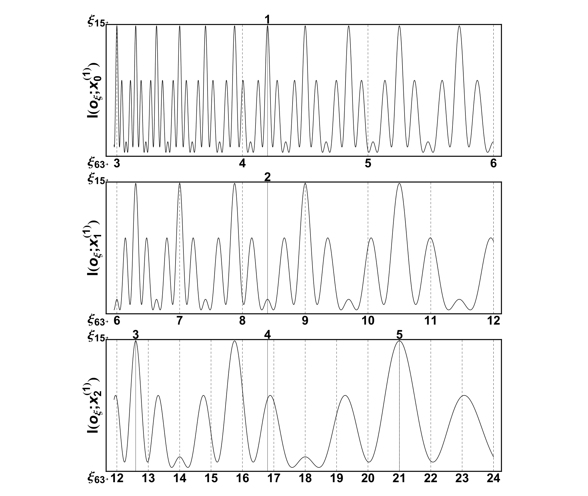
with , for each of the interferograms. We assume that our physical system is able to record such interferograms in the range . In Fig. we simulate these interferograms, which are able to cover all the trial factors in the interval for any integer in the range . An example is given for the factorization of by rescaling the axis as a function of and according to Eq. (13). The trial factors are marked, respectively, with continuous lines and dashed lines. We find the factors and of corresponding to maxima of the interferogram . On the other hand the factor of is associated with the maximum of the interferogram , while the factors and emerge from the maxima in the interferogram .
We consider now the method in Eq. (38). According to Eq. (50), any integer in the range can be factored by exploiting the same number
of interferograms defined by Eq. (3.1), with , where the value associated with the first interferogram satisfies the condition in Eq. (49)
| (54) |
From Eq. (13) we can now determine all the values
| (55) |
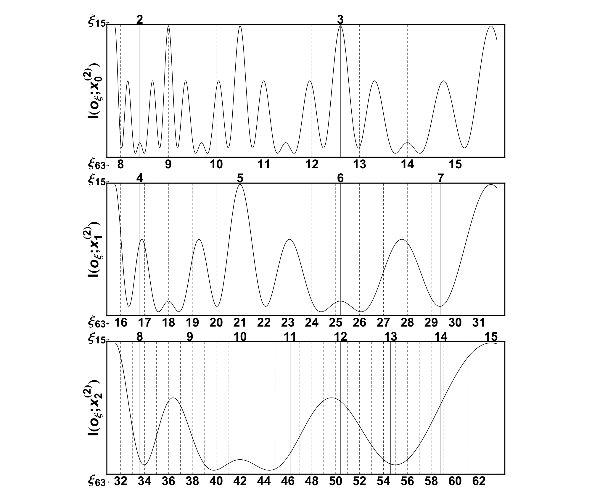
with , for each of the interferograms. We assume that our physical system covers the spectrum of values of a given observable . In Fig. we simulate such interferograms, which are able to cover all the trial factors in the interval for any integer in the range . We again give an example for the factorization of by rescaling the axis as a function of and according to Eq. (13). We find that the factor of corresponds to a maximum of the interferogram , while the factor is associated with a maximum of the interferogram . On the other hand the factor of is associated with the maximum of the interferogram .
 |
 |
4 Generalization of the CTES algorithm
In this section, we will introduce a generalization of the CTES algorithm. In particular, we generalize the scaling property defining the new auxiliary variable
| (56) |
where is equal to the product of one or more generic prime numbers (). We can now rescale the CTES function in Eq. (1) as a function of the continuous variable :
| (57) |
Let us describe how such a rescaled function allows us to find the factors of a generic number . If one of the chosen prime numbers that defines the value of is a factor of , we have solved the problem. If not, the factors of are the integer values of , different from the prime numbers that correspond to dominant maxima in the rescaled CTES function given by Eq. (57).
In a general analogue implementation, the auxiliary variable in Eq. (56) is obtained by rescaling the values of the observable according to
| (58) |
Thereby, the range of trial factors covered by the variable can be equivalent to the interval of trial factors covered by the variable by exploiting a range for the variable of the physical observable of length reduced by a factor . However, at the same time, each of the values , with , increases by the same factor according to the iteration formula (31) where in Eq. (49) now reads
| (59) |
with depending on the range (37) or (38), respectively, of trial factors we are considering. This implies that the maximum factorable integer is upper limited by , where is the maximum value physically allowed for the parameter .
5 Remarks
We have described a novel analogue algorithm based on the experimental measurement of CTES interferograms depending on the continuous argument and the discrete parameter associated with two suitable physical observables and , respectively. The domain of factorable integers is determined by the range of the continuous variable and by the maximum value allowed by the parameter .
The largest integer factorable with a single CTES interferogram associated with a given value of and defined in a certain range is upper limited by the value . For larger integers the available physical spectrum of observable values may not be enough to cover all the trail factors either in the range or . For this reason, we have introduced an algorithm based on the measurement of different interferograms , with , associated with the respective values . In this case the largest number factorable is upper limited by the value . We have demonstrated that the number of necessary experimental runs scales logarithmically with respect to the root of the number we want to factor. Very interestingly our method allows a parallel factorization of an exponential number of large integers with respect to the number of binary digits associated with . These results are very important in view of the optical implementation of the algorithm described in Ref. [5].
Moreover, we have introduced a generalized CTES procedure defined by the scaling property , where with generic prime numbers which are non factors of . We have shown that it is possible to reduce for a factor the length of the range of values in which the function is recorded. In such a case, the maximum factorable integer is upper limited by .
In Ref. [5], we describe in detail how an optical computer enables a physical computation of the CTES algorithm for several orders . In such a case the values and defining the analogue interferogram correspond, respectively, to the wavelengths of a polychromatic source and to the unit of displacement defining the optical paths in a generalized Michelson interferometer [2]. Indeed, an experimental proof of the principle of the CTES algorithm has been performed in the case of and , leading to the factorization of seven-digit numbers [5, 3].
6 Towards a polynomial scaling in the number of physical resources
We point out that any “classical” implementation of the algorithm described so far would lack exponential speed-up. Indeed, the largest number factorable is upper limited either by the value or , depending on the use of a single interferogram or a sequence of interferograms.
Moreover, the accuracy in the variable in Eq. (11)
depends on the given experimental indeterminations and associated with the measurement of the observables and , respectively. This shows from Eqs. (8) and (9) that the unit defining the CTES interferograms in Eq. (3.1) needs to grow exponentially with respect to the number of bits associated with the largest number in the interval of integers to be factored.
The ability to resolve the maxima associated with factors from non factors for larger and larger integers [1] can be, in general, improved by implementing ”factoring” interferograms of either a larger order or with a larger number of interfering terms as can be inferred by the relative curlicue functions in Fig. .
Ultimately, only a “quantum” system able to encode such physical observables in a qubit representation in line with Shor’s algorithm would make it possible to avoid the requirement of exponentially large values for the observable . In particular, a crucial role in our algorithm is played by the hyperbolic function in Eq. (3) emerging from the ratio of the values and and characterizing the “factoring” CTES interferograms in Eq. (3.1). A “qubit” parallel representation of functions analogous to the curlicue function may lead to novel factoring algorithms based on a polynomial number of resources. Moreover, multi-qubit quantum interference may serve as an efficient tool to distinguish factors from non factors.
Acknowledgements.
We thank H. Zhang, X. He, Y.H. Shih and W. P. Schleich for their contributions on this topic and J. Franson, M. Freyberger, A. Garuccio, S. Lomonaco, R. Meyers, T. Pittman and M. H. Rubin for many fruitful discussions.References
- (1) V. Tamma, Theoretical and experimental study of a new algorithm for factoring numbers (ProQuest, ISBN 978-1243759092, 2010).
- (2) V. Tamma, H. Zhang, X. He, A. Garuccio and Y. Shih, J. Mod. Opt. 56, 2125-2132 (2009).
- (3) V. Tamma, H. Zhang, X. He, A. Garuccio, W. P. Schleich, and Y.H. Shih, Phys. Rev. A (R) 83, 020304 (2011).
- (4) V. Tamma, C.O. Alley, W.P. Schleich and Y.H. Shih, Found. Phys. 42, 111-121 (2012).
- (5) V. Tamma, “Analogue algorithm for parallel factorization of an exponential number of large integers: I. Optical Implementation” (submitted to Quantum Information Processing)
- (6) P. Shor, in Proc. of the 35th Annual Symposium on Foundations of Computer Science, Santa Fe, NM, Nov. 20-22, 1994, IEEE Computer Society Press, pp. 124-134
- (7) For experimental implementations of the Shor algorithm see L.M.K. Vandersypen, M. Steffen, G. Breyta, C.S. Yannoni, M.H. Sherwood, and I.L. Chuang, Nature (London) 414, 883 (2001); C.-Y. Lu, D. E. Browne, T. Yang, and J.-W. Pan, Phys. Rev. Lett. 99, 250504 (2007); B. P. Lanyon, T. J. Weinhold, N. K. Langord, M.Barbieri, D. F. James, A. Gilchrist, and A. G: White, Phys. Rev. Lett. 99, 250505 (2007).
- (8) S. J. Lomonaco, Jr., Quantum Computation: A Grand Mathematical Challenge for the Twenty-First Century and the Millennium, Proceedings of Symposia in Applied Mathematics (2002)
- (9) M. A. Nielsen and I.L. Chuang, Quantum Computation and Quantum Information, Cambridge Univ. Press (2000).
- (10) N. D. Mermin, Quantum Computer Science, Cambridge Univ. Press (2007).
- (11) See for example H. Maier, and W. P. Schleich, Prime numbers 101, A primer on number theory (Wiley, New York, 2010).
- (12) J.F. Clauser, and J.P. Dowling, Phys. Rev. A 53, 4587 (1996).
- (13) J. Summhammer, Phys. Rev. A 56, 4324 (1997).
- (14) S. Wölk, W. Merkel, W. P. Schleich, I. S. Averbukh, and B. Girard, New Journal of Physics 13, 103007 (2011)
- (15) W. Merkel, S. Wölk, W. P. Schleich, I. S. Averbukh, B. Girard, and G. G. Paulus, New Journal of Physics 13, 103008 (2011)
- (16) S. Wölk and W. P. Schleich, New Journal of Physics 14, 013049 (2012)
- (17) H. Mack, M. Bienert, F. Haug, M. Freyberger, and W. P. Schleich, Phys. Status Solidi B 233, 408–415 (2002)
- (18) W. Merkel, I.Sh. Averbukh, B. Girard, G.G. Paulus, and W.P. Schleich, Fortschr. Phys. 54, 856 (2006).
- (19) M. Stefanak, W. Merkel, W.P. Schleich, D. Haase, and H. Maier, New J. Phys 9, 370 (2007).
- (20) M. Stefanak, D. Haase, W. Merkel, M.S. Zubairy, and W.P. Schleich, J. Phys. A: Math. Theor. 41, 304024 (2008).
- (21) S. Wölk, C. Feiler and W: P. Schleich, J. Mod. Opt. 56, 2118-2124 (2009).
- (22) A. A. Rangelov, J. Phys. B: At. Mol. Opt. Phys. 42, 021002 (2009).
- (23) M. Mehring, K. Müller, I.Sh. Averbukh, W. Merkel, and W.P. Schleich, Phys. Rev. Lett. 98, 120502 (2007).
- (24) T.S. Mahesh, N. Rajendran, X. Peng, and D. Suter, Phys. Rev. A 75, 062303 (2007).
- (25) X. Peng and D. Suter, EPL 84, 40006 (2008).
- (26) D. Bigourd, B. Chatel, W.P. Schleich, and B. Girard, Phys. Rev. Lett. 100, 030202 (2008).
- (27) S. Weber, B. Chatel and B. Girard, EPL 83, 34008 (2008).
- (28) M. Gilowsky, T. Wendrich, T. Muller, Ch. Jentsch, W. Ertmer, E.M. Rasel and W.P. Schleich, Phys. Rev. Lett. 100, 030201 (2008).
- (29) M. Sadgrove, S. Kumar, and K. Nakagawa, Phys. Rev. Lett. 101, 180502 (2008)
- (30) M.V. Berry, Physica D 33, 26 (1988); M.V. Berry and J. Goldberg, Nonlinearity 1,1 (1988).