跳到论文正文
W Papers独立论文阅读器 arXiv:1505.04421 论文正文 计算阅读时间 · 0%
引用这篇论文根据当前论文元数据生成,正式投稿前建议核对。


License: arXiv.org perpetual non-exclusive license
arXiv:1505.04421v1 [math.NA] 17 May 2015

MIDDLE EAST TECHNICAL UNIVERSITY Ankara, Turkey


INSTITUTE OF APPLIED MATHEMATICS
http://iam.metu.edu.tr


Time-space adaptive discontinuous Galerkin method for advection-diffusion equations with non-linear reaction mechanism

Bülent Karasözen11 1 Department of Mathematics and Institute of Applied Mathematics, Middle East Technical University, 06800 Ankara, Turkey, email: bulent@metu.edu.tr, Murat Uzunca22 2 Department of Mathematics, Middle East Technical University, 06800 Ankara, Turkey, email: uzunca@metu.edu.tr

Abstract. In this work, we apply a time-space adaptive discontinuous Galerkin method using the elliptic reconstruction technique with a robust (in Péclet number) elliptic error estimator in space, for the convection dominated parabolic problems with non-linear reaction mechanisms. We derive a posteriori error estimators in the L∞​(L2)+L2​(H1)L^{\infty}(L^{2})+L^{2}(H^{1})-type norm using backward Euler in time and discontinuous Galerkin (symmetric interior penalty Galerkin (SIPG)) in space. Numerical results for advection dominated reactive transport problems in homogeneous and heterogeneous media demonstrate the performance of the time-space adaptive algorithm.

Keywords. Non-linear diffusion-convection reaction, Discontinuous Galerkin, Time-space adaptivity, Elliptic reconstruction, A posteriori error estimates

Preprint No. 2014-6

August 2014

1 Introduction

Advection-diffusion-reaction (ADR) equations are widely used for systems in chemical reaction problems. In the linear convection or advection dominated case, stabilized continuous finite elements and discontinuous Galerkin (DG) methods are capable of handling the nonphysical oscillations. On the other hand, in the non-linear stationary case, the non-linear reaction term produces sharp layers in addition to the spurious oscillations due to the convection. Thus, an accurate and efficient numerical resolution of such layers is a challenge as the exact location of the layers are not known a priori. In the non-stationary case, the resolution of such layers is more critical since the nature of the sharp layers may vary as time progresses. Recently, several stabilization and shock/discontinuity capturing techniques were developed for linear and non-linear steady-state problems [4]. In contrast to the stabilized continuous Galerkin finite element methods, DG methods produce stable discretizations without the need for stabilization parameters. The DG combines the best properties of the finite volume and continuous finite elements methods. Finite volume methods can only use lower degree polynomials, and continuous finite elements methods require higher regularity due to the continuity requirements. The DG method is in particular suitable for non-matching grids and hp (space and order) adaptivity, detecting sharp layers and singularities. They are easily adapted locally for nonconforming finite elements requiring less regularity. Higher order DG approximation can be easily used by hierarchical bases [6], and the convergence rates are limited by the consistency error which makes the DG suitable for complex fluid flows. The DG methods are robust with respect to the variation of the physical parameters like diffusion constant and permeability. The stability of the DG approximation retained by adjusting the penalty parameter to penalize the jumps at the interface of the elements. Various choices of the penalty parameter is suggested in the literature [8, 10, 11, 21]. A unified analysis of the interior penalty DG methods for elliptic PDEs are given in [1]. Other advantages of the DG methods are conservation of mass and fluxes and parallelization. Moreover, DG methods are better suited for adaptive strategies which are based on (residual-based) a posteriori error estimation. The disadvantages are the resulting larger and denser matrices and ill-conditioning with increasing degree of the discontinuous polynomials.

The main tool in this paper is the adaptivity applied to the DG discretized (in space) systems using (residual-based) a posteriori error estimates. The aim of the a posteriori estimates is to derive bounds between the known numerical solution and the unknown exact solution. For elliptic diffusion-convection-reaction equations, there are various studies applying adaptivity using a posteriori error estimates in the literature [9, 12, 13, 17], which are well-understood. In this paper, we derive a posteriori error estimates for semi-linear ADR problems using the well-know elliptic a posteriori estimates, by which in contrast to the standard energy techniques we do not need to try to adapt the estimates case by case in order to compare the exact solution with numerical solution directly. For this reason, we use the elliptic reconstruction technique in [14] which allows us to utilize available a posteriori estimates derived for elliptic equations to control the main part of the spatial error. The idea of the elliptic reconstruction technique is to construct an auxiliary solution whose difference to the numerical solution can be estimated by a known (elliptic) a posteriori estimate, and the constructed auxiliary solution satisfies a variant of the given problem with a right hand side which can be controlled in an optimal way. By this way, we are able to obtain results being optimal order in both L2​(H1)L^{2}(H^{1}) and L∞​(L2)L^{\infty}(L^{2})-type norms, while the results obtained by the standard energy methods are only optimal order in L2​(H1)L^{2}(H^{1})-type norms, but sub-optimal order in L∞​(L2)L^{\infty}(L^{2})-type norms. In [7], a posteriori error estimates in the L∞​(L2)+L2​(H1)L^{\infty}(L^{2})+L^{2}(H^{1})-type norm are derived for linear parabolic diffusion-convection-reaction equations using backward Euler in time and discontinuous Galerkin in space utilizing the elliptic reconstruction technique. In this paper, we extend the study in [7] in a similar way by deriving and implementing a posteriori error estimates in the L∞​(L2)+L2​(H1)L^{\infty}(L^{2})+L^{2}(H^{1})-type norm using backward Euler in time and discontinuous Galerkin (symmetric interior penalty (SIPG)) in space for the convection dominated parabolic problems with non-linear reaction mechanisms. To derive the a posteriori error estimates, we use the modification of the robust (in Péclet number) a posteriori error estimator in [17] for linear steady-state diffusion-convection-reaction equations to the steady-state diffusion-convection equations with non-linear reaction mechanisms utilizing the elliptic reconstruction technique [14].

Application of the adaptive discontinuous Galerkin methods and a posteriori error estimates to the problems in geoscience are reviewed recently in [9]. Most of the applications of DG methods in geoscience concern reactive transport with advection [3, 13, 18] and strong permeability contrasts such as layered reservoirs [21] or vanishing and varying diffusivity posing challenges in computations [15]. The permeability in heterogeneous porous and fractured media varies over orders of magnitude in space, which results in highly variable flow field, where the local transport is dominated by advection or diffusion [19]. Accurate and efficient numerical solution of the ADR equations to predict the macroscopic mixing, anomalous transport of the solutes and contaminants for a wide range of parameters like permeability and Péclet numbers, different flow velocities and reaction rates and reaction rates are challenging problems [19]. In order to resolve the complex flow patterns accurately, higher order time stepping methods like exponential time stepping methods are used [19]. We show here using time-space adaptive first order backward Euler and DG in space, the same results can be obtained.

The rest of this paper is organized as follows. In the next section, we introduce the function spaces and related norms which are used in our analysis, and the model problem with the assumptions to have unique solution. In Section 3, we give the symmetric discontinuous interior penalty Galerkin discretized semi-discrete system, and fully-discrete system using Backward Euler in time. The derivation of a posteriori error estimator is given in Section 4, first for steady-state problems (with proofs), then for parabolic problems utilizing the elliptic reconstruction technique. In Section 5, we state the adaptive algorithm procedure using the a posteriori error estimators derived in Section 4. The solution procedure of the fully-discrete system by Newton method and the structures of the arising matrix and vectors are discussed in Section 6. After demonstrating the performance of the algorithm by some numerical studies in Section 7, the paper ends with conclusions.

2 Model problem

Let Ω⊂ℝ2\Omega\subset\mathbb{R}^{2} be a bounded, open and convex domain with boundary ∂Ω\partial\Omega. For a Banach space XX, define the spaces Lp​(0,T,X)L^{p}(0,T;X)

‖v‖Lp​(0,T,X)\displaystyle\|v\|_{L^{p}(0,T;X)} =(∫0T‖v⁡(t)‖Xp​𝑑t)1/p<∞,for ​1≤p<+∞\displaystyle=\left(\int_{0}^{T}\|v(t)\|_{X}^{p}dt\right)^{1/p}<\infty\;,\qquad\text{for }1\leq p<+\infty
‖v‖L∞​(0,T,X)\displaystyle\|v\|_{L^{\infty}(0,T;X)} =esssup0≤t≤T​‖v⁡(t)‖X<∞,for ​p=+∞\displaystyle=\underset{0\leq t\leq T}{\text{esssup}}\|v(t)\|_{X}<\infty\;,\qquad\text{for }p=+\infty

Also define the space

H1​(0,T,X)={v∈L2​(0,T,X)|vt∈L2​(0,T,X)}.H^{1}(0,T;X)=\{v\in L^{2}(0,T;X)|\;v_{t}\in L^{2}(0,T;X)\}.

We denote by C⁡(0,T,X)C(0,T;X) and C0,1​(0,T,X)C^{0,1}(0,T;X), the spaces of continuous and Lipschitz-continuous functions v:[0,T]↦Xv:[0,T]\mapsto X, respectively, equipped with the norms

‖v‖C⁡(0,T,X)\displaystyle\|v\|_{C(0,T;X)} =max0≤t≤T​‖v⁡(t)‖X<∞\displaystyle=\underset{0\leq t\leq T}{\text{max}}\|v(t)\|_{X}<\infty
‖v‖C0,1​(0,T,X)\displaystyle\|v\|_{C^{0,1}(0,T;X)} =max​{‖v‖C⁡(0,T,X),‖vt‖C⁡(0,T,X)}<∞\displaystyle=\text{max}\left\{\|v\|_{C(0,T;X)},\|v_{t}\|_{C(0,T;X)}\right\}<\infty

We consider the system of semi-linear diffusion-convection-reaction equations

∂ui∂t−∇⋅(ϵi∇ui)+β→i⋅∇ui+ri(u→)=fi,i=1,2,…,J\frac{\partial u_{i}}{\partial t}-\nabla\cdot(\epsilon_{i}\nabla u_{i})+\vec{\beta}_{i}\cdot\nabla u_{i}+r_{i}(\vec{u})=f_{i}\;\;,\quad i=1,2,\ldots,J (3)

in Ω×(0,T]\Omega\times(0,T] for the vector of unknowns u→=(u1,u2,…,uJ)T\vec{u}=(u_{1},u_{2},\ldots,u_{J})^{T} with appropriate boundary and initial conditions. We assume that the source functions fi∈C⁡(0,T,L2​(Ω))f_{i}\in C(0,T;L^{2}(\Omega)), and the velocity fields β→i∈C​(0,T,W1,∞​(Ω))2\vec{\beta}_{i}\in C\left(0,T;W^{1,\infty}(\Omega)\right)^{2} either given or computed. For flow in heterogeneous media in Section 7.4, the symmetric dispersion tensors ϵi\epsilon_{i} are taken of the form

ϵi=[Di100Di2]\epsilon_{i}=\begin{bmatrix}D_{i}^{1}&0\\ 0&D_{i}^{2}\end{bmatrix}

with 0<Di1,Di2≪10<D_{i}^{1},D_{i}^{2}\ll 1. Moreover, we assume that the non-linear reaction terms are bounded, locally Lipschitz continuous and monotone, i.e. satisfies for any s,s1,s2≥0s,s_{1},s_{2}\geq 0, s,s1,s2∈ℝs,s_{1},s_{2}\in\mathbb{R} the following conditions [20]

|ri​(s)|\displaystyle|r_{i}(s)| ≤Cs,Cs>0\displaystyle\leq C_{s},\quad C_{s}>0 (4a)
‖ri​(s1)−ri​(s2)‖L2​(Ω)\displaystyle\|r_{i}(s_{1})-r_{i}(s_{2})\|_{L^{2}(\Omega)} ≤L​‖s1−s2‖L2​(Ω),L>0\displaystyle\leq L\|s_{1}-s_{2}\|_{L^{2}(\Omega)},\quad L>0 (4b)
ri∈C1​(ℝ0+),ri​(0)=0,\displaystyle r_{i}\in C^{1}(\mathbb{R}_{0}^{+}),\quad r_{i}(0)=0, ri′​(s)≥0.\displaystyle\quad r_{i}^{\prime}(s)\geq 0. (4c)

We also assume that there are κ,κ∗≥0\kappa,\kappa_{*}\geq 0 satisfying for i=1,2,…,Ji=1,2,\ldots,J

−12∇⋅β→i(x)≥κ,∥−∇⋅β→i∥C⁡(0,T,L∞​(Ω))≤κ∗κ,-\frac{1}{2}\nabla\cdot\vec{\beta}_{i}(x)\geq\kappa,\qquad\|-\nabla\cdot\vec{\beta}_{i}\|_{C(0,T;L^{\infty}(\Omega))}\leq\kappa^{*}\kappa, (5)

The first inequality in (5) ensures the well-posedness of the problem, and the letter is used in the a posteriori error analysis.

The weak formulation of the system (3) reads as: for any v∈H01​(Ω)v\in H_{0}^{1}(\Omega), find ui∈L2​(0,T,H01​(Ω))∩H1​(0,T,L2​(Ω))u_{i}\in L^{2}(0,T;H_{0}^{1}(\Omega))\cap H^{1}(0,T;L^{2}(\Omega)), i=1,2,…,Ji=1,2,\ldots,J, such that for all t∈(0,T]t\in(0,T]

∫Ω∂ui∂t​v​𝑑x+a⁡(t,ui,v)+bi​(t,u→,v)=li​(v)\int_{\Omega}\frac{\partial u_{i}}{\partial t}vdx+a(t;u_{i},v)+b_{i}(t;\vec{u},v)=l_{i}(v) (6)
a⁡(t,ui,v)=\displaystyle a(t;u_{i},v)= ∫Ω(ϵi∇ui⋅∇v+β→i⋅∇uiv)dx,\displaystyle\int_{\Omega}(\epsilon_{i}\nabla u_{i}\cdot\nabla v+\vec{\beta}_{i}\cdot\nabla u_{i}v)dx, (7a)
bi​(t,u→,v)=\displaystyle b_{i}(t;\vec{u},v)= ∫Ωri​(u→)​v​𝑑x,\displaystyle\int_{\Omega}r_{i}(\vec{u})vdx, (7b)
li​(v)=\displaystyle l_{i}(v)= ∫Ωfi​v​𝑑x\displaystyle\int_{\Omega}f_{i}vdx (7c)

which have unique solutions {ui}i=1J\{u_{i}\}_{i=1}^{J} in the space C​(0,T,L2​(Ω))C(0,T;L^{2}(\Omega)) under the given regularity assumptions and the conditions (4a)-(4c).

In the sequel, for simplicity, we just consider a single equation of the system (3) (J=1) without any subscript to construct the discontinuous Galerkin discretization in the next section and thereafter, and we also continue with a homogeneous dispersion tensor leading to a simple diffusivity constant 0<ϵ≪10<\epsilon\ll 1. We, furthermore, take into account the homogeneous Dirichlet boundary conditions to simplify the notations. It can be proceeded with heterogeneous dispersion tensor and other type of boundary conditions in a standard way.

3 Discontinuous Galerkin discretization

For space discretization of a single equation of (3), we use the symmetric discontinuous interior penalty Galerkin (SIPG) method [1, 16] with the upwinding for the convection part [2, 12].

Let {ξh}\{\xi_{h}\} be a family of shape regular meshes with the elements (triangles) Ki∈ξhK_{i}\in\xi_{h} satisfying Ω¯=∪K¯\overline{\Omega}=\cup\overline{K} and Ki∩Kj=∅K_{i}\cap K_{j}=\emptyset for KiK_{i}, KjK_{j} ∈ξh\in\xi_{h}. Let us denote by Γ0\Gamma^{0} and Γ∂\Gamma^{\partial} the set of interior and Dirichlet boundary edges, respectively, so that Γ=Γ0∪Γ∂\Gamma=\Gamma^{0}\cup\Gamma^{\partial} forms the skeleton of the mesh. For any K∈ξhK\in\xi_{h}, let ℙk​(K)\mathbb{P}_{k}(K) be the set of all polynomials of degree at most kk on KK. Then, set the finite dimensional space

Vh(ξh)={v∈L2(Ω):v|K∈ℙk(K),∀K∈ξh}⊄H01(Ω).V_{h}(\xi_{h})=\left\{v\in L^{2}(\Omega):v|_{K}\in\mathbb{P}_{k}(K),\;\forall K\in\xi_{h}\right\}\not\subset H_{0}^{1}(\Omega).

The functions in Vh​(ξh)V_{h}(\xi_{h}), in contrast to the standard (continuous) finite elements, are discontinuous along the inter-element boundaries causing that along an interior edge, there are two different traces from the adjacent elements sharing that edge. In the light of this fact, let us first introduce some notations before giving the SIPG formulation. Let KiK_{i}, Kj∈ξhK_{j}\in\xi_{h} (i<ji<j) be two adjacent elements sharing an interior edge e=Ki∩Kj⊂Γ0e=K_{i}\cap K_{j}\subset\Gamma_{0} (see Fig.1). We denote the trace of a scalar function vv from inside KiK_{i} by viv_{i} and from inside KjK_{j} by vjv_{j}, and then we set the jump and average values of vv on the edge ee

[v]=vi​n→e−vj​n→e,{v}=12​(vi+vj).[v]=v_{i}\vec{n}_{e}-v_{j}\vec{n}_{e},\quad\{v\}=\frac{1}{2}(v_{i}+v_{j}).

Here n→e\vec{n}_{e} denotes the unit normal to the edge ee oriented from KiK_{i} to KjK_{j}. Similarly, we set the jump and average values of a vector valued function q→\vec{q} on e

[q→]=q→i⋅n→e−q→j⋅n→e,{q→}=12​(q→i+q→j),[\vec{q}]=\vec{q}_{i}\cdot\vec{n}_{e}-\vec{q}_{j}\cdot\vec{n}_{e},\quad\{\vec{q}\}=\frac{1}{2}(\vec{q}_{i}+\vec{q}_{j}),

Observe that [v][v] is a vector for a scalar function vv, while, [q→][\vec{q}] is scalar for a vector valued function q→\vec{q}. On the other hand, along any boundary edge e=Ki∩∂Ωe=K_{i}\cap\partial\Omega, we set

[v]=vi​n→,{v}=vi,[q→]=q→i⋅n→,{q→}=q→i[v]=v_{i}\vec{n},\quad\{v\}=v_{i},\quad[\vec{q}]=\vec{q}_{i}\cdot\vec{n},\quad\{\vec{q}\}=\vec{q}_{i}

where n→\vec{n} is the unit outward normal to the boundary at ee. We define the inflow and outflow boundary parts at a time tt by

Γt−={x∈∂Ω|β→​(x→,t)⋅n→​(x)<0},Γt+=∂Ω∖Γt−\Gamma_{t}^{-}=\{x\in\partial\Omega|\;\vec{\beta}(\vec{x},t)\cdot\vec{n}(x)<0\}\;,\qquad\Gamma_{t}^{+}=\partial\Omega\setminus\Gamma_{t}^{-}

At a time tt, the inflow and outflow parts of an element KK are defined by

∂Kt−={x∈∂K|β→​(x→,t)⋅n→K​(x)<0},∂Kt+=∂K∖∂Kt−\partial K_{t}^{-}=\{x\in\partial K|\;\vec{\beta}(\vec{x},t)\cdot\vec{n}_{K}(x)<0\}\;,\qquad\partial K_{t}^{+}=\partial K\setminus\partial K_{t}^{-}

where n→K​(x)\vec{n}_{K}(x) denotes the outward unit normal to the boundary of the element KK at xx.

K i K j e → n e K i ∂ Ω e → n
Figure 1: Two adjacent elements sharing an edge (left); an element near to domain boundary (right)

Under the given definitions, the semi-discrete problem reads as: for t=0t=0, set uh​(0)∈Vh​(ξh)u_{h}(0)\in V_{h}(\xi_{h}) as the projection (orthogonal L2L^{2}-projection) of u0u_{0} onto Vh​(ξh)V_{h}(\xi_{h}); for each t∈(0,T]t\in(0,T], for all vh∈Vh​(ξh)v_{h}\in V_{h}(\xi_{h}), find uh∈C0,1​(0,T,Vh​(ξh))u_{h}\in C^{0,1}(0,T;V_{h}(\xi_{h})) such that

∫Ω∂uh∂t​vh​𝑑x+ah​(t,uh,vh)+Kh​(uh,vh)+bh​(t,uh,vh)=lh​(vh),\int_{\Omega}\frac{\partial u_{h}}{\partial t}v_{h}dx+a_{h}(t;u_{h},v_{h})+K_{h}(u_{h},v_{h})+b_{h}(t;u_{h},v_{h})=l_{h}(v_{h}), (8)
ah​(t,uh,vh)=\displaystyle a_{h}(t;u_{h},v_{h})= ∑K∈ξh∫Kϵ∇uh⋅∇vhdx+∑K∈ξh∫Kβ→⋅∇uhvhdx\displaystyle\sum\limits_{K\in{\xi}_{h}}\int_{K}\epsilon\nabla u_{h}\cdot\nabla v_{h}dx+\sum\limits_{K\in{\xi}_{h}}\int_{K}\vec{\beta}\cdot\nabla u_{h}v_{h}dx (9a)
+∑K∈ξh∫∂Kt−∖∂Ωβ→⋅n→K(uho​u​t−uh)vhds−∑K∈ξh∫∂Kt−∩Γt−β→⋅n→Kuhvhds\displaystyle+\sum\limits_{K\in{\xi}_{h}}\int_{\partial K_{t}^{-}\setminus\partial\Omega}\vec{\beta}\cdot\vec{n}_{K}(u_{h}^{out}-u_{h})v_{h}ds-\sum\limits_{K\in{\xi}_{h}}\int_{\partial K_{t}^{-}\cap\Gamma_{t}^{-}}\vec{\beta}\cdot\vec{n}_{K}u_{h}v_{h}ds
+∑e∈Γσ​ϵhe∫e[uh]⋅[vh]ds,\displaystyle+\sum\limits_{e\in\Gamma}\frac{\sigma\epsilon}{h_{e}}\int_{e}[u_{h}]\cdot[v_{h}]ds,
Kh​(uh,vh)=\displaystyle K_{h}(u_{h},v_{h})= −∑e∈Γ∫e({ϵ∇vh}⋅[uh]+{ϵ∇uh}⋅[vh])ds\displaystyle-\sum\limits_{e\in\Gamma}\int_{e}(\{\epsilon\nabla v_{h}\}\cdot[u_{h}]+\{\epsilon\nabla u_{h}\}\cdot[v_{h}])ds (9b)
bh​(t,uh,vh)=\displaystyle b_{h}(t;u_{h},v_{h})= ∑K∈ξh∫Kr⁡(uh)​vh​𝑑x,\displaystyle\sum\limits_{K\in{\xi}_{h}}\int_{K}r(u_{h})v_{h}dx, (9c)
lh​(vh)=\displaystyle l_{h}(v_{h})= ∑K∈ξh∫Kfh​vh​𝑑x\displaystyle\sum\limits_{K\in{\xi}_{h}}\int_{K}f_{h}v_{h}dx (9d)

where uho​u​tu_{h}^{out} denotes the value on an edge from outside of an element KK. The parameter σ∈ℝ0+\sigma\in\mathbb{R}_{0}^{+} is called the penalty parameter which should be sufficiently large; independent of the mesh size hh and the diffusion coefficient ϵ\epsilon [16] [Sec. 2.7.1]. We choose the penalty parameter σ\sigma for the SIPG method depending on the polynomial degree kk as σ=3​k​(k+1)\sigma=3k(k+1) on interior edges and σ=6​k​(k+1)\sigma=6k(k+1) on boundary edges.

Upon integration by parts on the convective term, bilinear form (9a) will be

ah​(t,uh,vh)=\displaystyle a_{h}(t;u_{h},v_{h})= ∑K∈ξh∫Kϵ∇uh⋅∇vhdx−∑K∈ξh∫K(β→uh⋅∇vh+∇⋅β→uhvh)dx\displaystyle\sum\limits_{K\in{\xi}_{h}}\int_{K}\epsilon\nabla u_{h}\cdot\nabla v_{h}dx-\sum\limits_{K\in{\xi}_{h}}\int_{K}(\vec{\beta}u_{h}\cdot\nabla v_{h}+\nabla\cdot\vec{\beta}u_{h}v_{h})dx (10a)
+∑K∈ξh∫∂Kt+∖∂Ωβ→⋅n→Kuh(vh−vho​u​t)ds+∑K∈ξh∫∂Kt+∩Γt+β→⋅n→Kuhvhds\displaystyle+\sum\limits_{K\in{\xi}_{h}}\int_{\partial K_{t}^{+}\setminus\partial\Omega}\vec{\beta}\cdot\vec{n}_{K}u_{h}(v_{h}-v_{h}^{out})ds+\sum\limits_{K\in{\xi}_{h}}\int_{\partial K_{t}^{+}\cap\Gamma_{t}^{+}}\vec{\beta}\cdot\vec{n}_{K}u_{h}v_{h}ds
+∑e∈Γσ​ϵhe∫e[uh]⋅[vh]ds\displaystyle+\sum\limits_{e\in\Gamma}\frac{\sigma\epsilon}{h_{e}}\int_{e}[u_{h}]\cdot[v_{h}]ds

Note that the bilinear form ah​(t,u,v)a_{h}(t;u,v) is well-defined for the functions u,v∈H01​(Ω)u,v\in H_{0}^{1}(\Omega), and equal to

ah(t;u,v)=∫Ω(ϵ∇u⋅∇v+β→⋅∇uv)dxa_{h}(t;u,v)=\int_{\Omega}(\epsilon\nabla u\cdot\nabla v+\vec{\beta}\cdot\nabla uv)dx

Thus, the weak formulation (7a) can be rewritten for any t∈(0,T]t\in(0,T] as

∫Ω∂u∂t​v​𝑑x+ah​(t,u,v)+b⁡(t,u,v)=l⁡(v),∀v∈H01​(Ω)\int_{\Omega}\frac{\partial u}{\partial t}vdx+a_{h}(t;u,v)+b(t;u,v)=l(v)\;,\qquad\forall v\in H_{0}^{1}(\Omega) (11)

For the fully discrete system, consider a subdivision of [0,T][0,T] into nn time intervals Ik=(tk−1,tk]I_{k}=(t^{k-1},t^{k}] of length τk\tau_{k}, k=1,2,…,nk=1,2,\ldots,n. Set t0=0t^{0}=0 and for n≥1n\geq 1, tk=τ1+τ2+⋯+τkt^{k}=\tau_{1}+\tau_{2}+\cdots+\tau_{k}. Denote by ξh0\xi_{h}^{0} an initial mesh and by ξhk\xi_{h}^{k} the mesh associated to the kt​hk^{th} time step for k>0k>0, which is obtained from ξhk−1\xi_{h}^{k-1} by locally refining/coarsening. Moreover, we assign the finite element space Vhk=Vh​(ξhk)V_{h}^{k}=V_{h}(\xi_{h}^{k}) to each mesh ξhk\xi_{h}^{k}. Then, the fully discrete problem, backward Euler in time, reads as: for t=0t=0, set uh0∈Vh0u_{h}^{0}\in V_{h}^{0} as the projection (orthogonal L2L^{2}-projection) of u0u_{0} onto Vh0V_{h}^{0}; for k=1,2,…,nk=1,2,\ldots,n, find uhk∈Vhku_{h}^{k}\in V_{h}^{k} such that for all vhk∈Vhkv_{h}^{k}\in V_{h}^{k}

∫Ωuhk−uhk−1τk​vhk​𝑑x+ah​(tk,uhk,vhk)+Kh​(uhk,vhk)+bh​(tk,uhk,vhk)=∫Ωfk​vhk​𝑑x\int_{\Omega}\frac{u_{h}^{k}-u_{h}^{k-1}}{\tau_{k}}v_{h}^{k}dx+a_{h}(t^{k};u_{h}^{k},v_{h}^{k})+K_{h}(u_{h}^{k},v_{h}^{k})+b_{h}(t^{k};u_{h}^{k},v_{h}^{k})=\int_{\Omega}f^{k}v_{h}^{k}dx (12)

4 A posteriori error analysis

The problems concerned in this paper are convection/reaction dominated non-stationary models which often produce internal/boundary layers where the solutions have steep gradients. Thus, an efficient solution of such equations are needed. The most popular technique to solve the convection/reaction dominated problems is the adaptivity which requires an estimator to locate the regions where the error is too large. In this work, we construct the residual-based, robust (in Péclet number) a posteriori error estimators for non-stationary convection domianted diffusion-convection equations with non-linear reaction mechanisms. To construct the a posteriori error estimators, we extend the a posteriori error estimators for linear non-stationary problems constructed in [7] which uses the a posteriori error estimators for linear stationary models constructed in [17] utilizing the elliptic reconstruction technique [14] to make connection between the stationary and non-stationary error. As in [7], first we construct and prove the a posteriori error bounds for non-linear stationary models in Section 4.1. Then, in Section 4.2, we give the a posteriori error bounds for the semi-discrete system of the non-stationary problems with non-linear reaction term. Finally, in Section 4.3, we give the a posteriori error bounds for the fully-discrete system of the non-stationary problems with non-linear reaction term. The main contribution to the error analysis lies in the construction of the error bounds for non-linear stationary models in Section 4.1. The remaining utilize the constructions in [7].

4.1 A posteriori error bounds for non-linear stationary system

We consider first the stationary problem, i.e. for a given t∈(0,T]t\in(0,T], let us∈H01​(Ω)u^{s}\in H_{0}^{1}(\Omega) be the unique solution to the weak problem

a⁡(t,us,v)+b⁡(t,us,v)=l⁡(v),∀v∈H01​(Ω)a(t;u^{s},v)+b(t;u^{s},v)=l(v)\;,\qquad\forall v\in H_{0}^{1}(\Omega) (13)

and let uhs∈Vh​(ξh)u_{h}^{s}\in V_{h}(\xi_{h}) be the unique solution to the discrete problem

ah​(t,uhs,vh)+Kh​(uhs,vh)+bh​(t,uhs,vh)=l⁡(vh),∀v∈Vh​(ξh)a_{h}(t;u_{h}^{s},v_{h})+K_{h}(u_{h}^{s},v_{h})+b_{h}(t;u_{h}^{s},v_{h})=l(v_{h})\;,\qquad\forall v\in V_{h}(\xi_{h}) (14)

In order to measure the spatial error, we use the energy norm

|||v|||2=∑K∈ξh(∥ϵ∇v∥L2​(K)2+κ∥v∥L2​(K)2)+∑e∈Γϵ​σhe∥[v]∥L2​(e)2,|||v|||^{2}=\sum\limits_{K\in{\xi}_{h}}(\|\epsilon\nabla v\|_{L^{2}(K)}^{2}+\kappa\|v\|_{L^{2}(K)}^{2})+\sum\limits_{e\in\Gamma}\frac{\epsilon\sigma}{h_{e}}\|[v]\|_{L^{2}(e)}^{2},

and the semi-norm

|v|C2=|β→​v|∗2+∑e∈Γ(κ​he+heϵ)​‖[v]‖L2​(e)2,|v|_{C}^{2}=|\vec{\beta}v|_{*}^{2}+\sum\limits_{e\in\Gamma}(\kappa h_{e}+\frac{h_{e}}{\epsilon})\|[v]\|_{L^{2}(e)}^{2}, (15)

where

|u|∗=supw∈H01​(Ω)∖{0}⁡∫Ωu⋅∇w​𝑑x‖|w|‖,|u|_{*}=\mathop{\text{sup}}_{w\in H_{0}^{1}(\Omega)\setminus\{0\}}\frac{\int_{\Omega}u\cdot\nabla wdx}{|||w|||},

For each element K∈ξhK\in{\xi}_{h}, we define the local error indicators ηK2\eta_{K}^{2} as

ηK2=ηRK2+ηEK2+ηJK2,\displaystyle\eta_{K}^{2}=\eta_{R_{K}}^{2}+\eta_{E_{K}}^{2}+\eta_{J_{K}}^{2}, (16)

where

ηRK2\displaystyle\eta_{R_{K}}^{2} =\displaystyle= ρK2​‖fh+ϵ​Δ​uhs−β→h⋅∇uhs−r⁡(uhs)‖L2​(K)2,\displaystyle\rho_{K}^{2}\|f_{h}+\epsilon\Delta u_{h}^{s}-\vec{\beta}_{h}\cdot\nabla u_{h}^{s}-r(u_{h}^{s})\|_{L^{2}(K)}^{2},
ηEK2\displaystyle\eta_{E_{K}}^{2} =\displaystyle= 12∑e∈∂K∖Γ∂ϵ−12ρe∥[ϵ∇uhs]∥L2​(e)2,\displaystyle\frac{1}{2}\sum\limits_{e\in\partial K\setminus\Gamma^{\partial}}\epsilon^{-\frac{1}{2}}\rho_{e}\|[\epsilon\nabla u_{h}^{s}]\|_{L^{2}(e)}^{2},
ηJK2\displaystyle\eta_{J_{K}}^{2} =\displaystyle= 12​∑e∈∂K∖Γ∂(ϵ​σhe+κ​he+heϵ)​‖[uhs]‖L2​(e)2+∑e∈∂K∩Γ∂(ϵ​σhe+κ​he+heϵ)​‖uhs‖L2​(e)2,\displaystyle\frac{1}{2}\sum\limits_{e\in\partial K\setminus\Gamma^{\partial}}\left(\frac{\epsilon\sigma}{h_{e}}+\kappa h_{e}+\frac{h_{e}}{\epsilon}\right)\|[u_{h}^{s}]\|_{L^{2}(e)}^{2}+\sum\limits_{e\in\partial K\cap\Gamma^{\partial}}\left(\frac{\epsilon\sigma}{h_{e}}+\kappa h_{e}+\frac{h_{e}}{\epsilon}\right)\|u_{h}^{s}\|_{L^{2}(e)}^{2},

with the weights ρK\rho_{K} and ρe\rho_{e}, on an element KK, given by

ρK=min⁡{hK​ϵ−12,κ−12},ρe=min⁡{he​ϵ−12,κ−12},\rho_{K}=\min\{h_{K}\epsilon^{-\frac{1}{2}},\kappa^{-\frac{1}{2}}\},\;\rho_{e}=\min\{h_{e}\epsilon^{-\frac{1}{2}},\kappa^{-\frac{1}{2}}\},

for κ≠0\kappa\neq 0. When κ=0\kappa=0, we take ρK=hK​ϵ−12\rho_{K}=h_{K}\epsilon^{-\frac{1}{2}} and ρe=he​ϵ−12\rho_{e}=h_{e}\epsilon^{-\frac{1}{2}}. Then, our a posteriori error indicator is given by

η=(∑K∈ξhηK2)1/2.\eta=\left(\sum\limits_{K\in{\xi}_{h}}\eta_{K}^{2}\right)^{1/2}. (18)

We also introduce the data approximation terms,

ΘK2=ρK2​(‖f−fh‖L2​(K)2+‖(β→−β→h)⋅∇uhs‖L2​(K)2).\Theta_{K}^{2}=\rho_{K}^{2}(\|f-f_{h}\|_{L^{2}(K)}^{2}+\|(\vec{\beta}-\vec{\beta}_{h})\cdot\nabla u_{h}^{s}\|_{L^{2}(K)}^{2}).

and the data approximation error

Θ=(∑K∈ξhΘK2)1/2.\Theta=\left(\sum\limits_{K\in{\xi}_{h}}\Theta_{K}^{2}\right)^{1/2}. (19)

Then, we have the a posteriori error bounds

‖us−uhs‖D​G≲η+Θ\displaystyle\|u^{s}-u_{h}^{s}\|_{DG}\lesssim\eta+\Theta\qquad (reliability),\displaystyle(\text{reliability}), (20)
η≲‖us−uhs‖D​G+Θ\displaystyle\eta\lesssim\|u^{s}-u_{h}^{s}\|_{DG}+\Theta\qquad (efficiency).\displaystyle(\text{efficiency}). (21)

with

‖v‖D​G=‖|v|‖+|v|C\|v\|_{DG}=|||v|||+|v|_{C}

4.1.1 Proof of a posteriori error bounds

The proof for the bounds of spatial error estimates are analogous to the ones in [17] for the linear problems. Therefore, only the proofs for non-linear reaction term are stated explicitly . In the following, we use the symbols ≲\lesssim and ≳\gtrsim to denote the bounds that are valid up to positive constants independent of the local mesh size hh, the diffusion coefficient ϵ\epsilon and the penalty parameter σ\sigma.

The spatial error ‖us−uhs‖D​G\|u^{s}-u_{h}^{s}\|_{DG} is not well-defined, since us∈H01​(Ω)u^{s}\in H_{0}^{1}(\Omega) and uhs∈Vh​(ξh)⊈H01​(Ω)u_{h}^{s}\in V_{h}(\xi_{h})\nsubseteq H_{0}^{1}(\Omega). Therefore, we split the stationary SIPG solution uhsu_{h}^{s} as

uhs=uhc+uhru_{h}^{s}=u_{h}^{c}+u_{h}^{r}

with uhc∈H01​(Ω)∩Vh​(ξh)u_{h}^{c}\in H_{0}^{1}(\Omega)\cap V_{h}(\xi_{h}) being the conforming part of the solution and uhr∈Vh​(ξh)u_{h}^{r}\in V_{h}(\xi_{h}) is the remainder term. In this way, we have uhs∈H01​(Ω)+Vh​(ξh)u_{h}^{s}\in H_{0}^{1}(\Omega)+V_{h}(\xi_{h}), and from the triangular inequality

‖us−uhs‖D​G≤‖us−uhc‖D​G+‖uhr‖D​G\|u^{s}-u_{h}^{s}\|_{DG}\leq\|u^{s}-u_{h}^{c}\|_{DG}+\|u_{h}^{r}\|_{DG}

Now, both the terms on the right hand side are well-defined norms, and our aim is to find bounds for them. Next, we introduce the following auxiliary forms:

Dh​(u,v)=\displaystyle D_{h}(u,v)= ∑K∈ξh∫K(ϵ∇u⋅∇v−∇⋅β→uv)dx\displaystyle\sum\limits_{K\in{\xi}_{h}}\int_{K}\left(\epsilon\nabla u\cdot\nabla v-\nabla\cdot\vec{\beta}uv\right)dx (22a)
Oh​(u,v)=\displaystyle O_{h}(u,v)= −∑K∈ξh∫Kβ→u⋅∇vdx+∑K∈ξh∫∂K+∩Γ+β→⋅n→Kuvds\displaystyle-\sum\limits_{K\in{\xi}_{h}}\int_{K}\vec{\beta}u\cdot\nabla vdx+\sum\limits_{K\in{\xi}_{h}}\int_{\partial K^{+}\cap\Gamma^{+}}\vec{\beta}\cdot\vec{n}_{K}uvds
+∑K∈ξh∫∂K+∖∂Ωβ→⋅n→Ku(v−vo​u​t)ds\displaystyle+\sum\limits_{K\in{\xi}_{h}}\int_{\partial K^{+}\setminus\partial\Omega}\vec{\beta}\cdot\vec{n}_{K}u(v-v^{out})ds (22b)
Jh​(u,v)=\displaystyle J_{h}(u,v)= ∑e∈Γ0∪Γσ​ϵhe​∫e[u]⋅[v]​𝑑s.\displaystyle\sum\limits_{e\in\Gamma_{0}\cup\Gamma}\frac{\sigma\epsilon}{h_{e}}\int_{e}[u]\cdot[v]ds. (22c)

We note that, for a specific t∈(0,T]t\in(0,T], the SIPG bilinear form (10a) satisfies

ah​(t,u,v)=Dh​(u,v)+Oh​(u,v)+Jh​(u,v)a_{h}(t;u,v)=D_{h}(u,v)+O_{h}(u,v)+J_{h}(u,v)

and is well-defined on H01​(Ω)+Vh​(ξh)H_{0}^{1}(\Omega)+V_{h}(\xi_{h}). Using the first identity in (5), we can easily have for any u∈H01​(Ω)u\in H_{0}^{1}(\Omega)

ah​(t,u,v)≥‖|u|‖2{a}_{h}(t;u,v)\geq|||u|||^{2}

Moreover, the auxiliary forms are continuous [17][Lemma 4.2]:

|Dh​(u,v)|\displaystyle|D_{h}(u,v)| ≲\displaystyle\lesssim ‖|u|‖​‖|v|‖,u,v∈H01​(Ω)+Vh​(ξh),\displaystyle|||u|||\;|||v|||\;,\qquad u,v\in H_{0}^{1}(\Omega)+V_{h}(\xi_{h}), (23)
|Oh​(u,v)|\displaystyle|O_{h}(u,v)| ≲\displaystyle\lesssim |β→​u|∗​‖|v|‖,u∈H01​(Ω)+Vh​(ξh),v∈H01​(Ω),\displaystyle|\vec{\beta}u|_{*}\;|||v|||\;,\qquad u\in H_{0}^{1}(\Omega)+V_{h}(\xi_{h}),v\in H_{0}^{1}(\Omega), (24)
|Jh​(u,v)|\displaystyle|J_{h}(u,v)| ≲\displaystyle\lesssim ‖|u|‖​‖|v|‖,u,v∈H01​(Ω)+Vh​(ξh),\displaystyle|||u|||\;|||v|||\;,\qquad u,v\in H_{0}^{1}(\Omega)+V_{h}(\xi_{h}), (25)

and for u∈Vh​(ξh)u\in V_{h}(\xi_{h}), v∈Vh​(ξh)∩H01​(Ω)v\in V_{h}(\xi_{h})\cap H_{0}^{1}(\Omega) [17][Lemma 4.3]

|Kh​(u,v)|\displaystyle|K_{h}(u,v)| ≲\displaystyle\lesssim γ−1/2(∑e∈Γ0∪ΓDγ​ϵhe∥[u]∥L2​(e))1/2|||v|||.\displaystyle\gamma^{-1/2}\left(\sum_{e\in\Gamma_{0}\cup\Gamma^{D}}\frac{\gamma\epsilon}{h_{e}}\|[u]\|_{L^{2}(e)}\right)^{1/2}|||v|||. (26)

We also have for the non-linear form bh​(t,u,v)b_{h}(t;u,v), for a specific time tt, using the boundedness assumption (4a),

|bh​(t,u,v)|\displaystyle|b_{h}(t;u,v)| ≲\displaystyle\lesssim ‖|v|‖,u,v∈H01​(Ω)+Vh​(ξh).\displaystyle|||v|||\;,\qquad u,v\in H_{0}^{1}(\Omega)+V_{h}(\xi_{h}). (27)

Now, we give some auxiliary results and conditions which are used in the proofs.

  • •

    Inf-sup condition: [17][Lemma 4.4] For a nonzero u∈H01​(Ω)u\in H_{0}^{1}(\Omega), for a constant C>0C>0, we have

    ‖|u|‖+|β→​u|∗≲supv∈H01​(Ω)∖{0}​ah​(t,u,v)‖|v|‖.\displaystyle|||u|||+|\vec{\beta}u|_{*}\lesssim\underset{v\in H_{0}^{1}(\Omega)\setminus\{0\}}{\text{sup}}\frac{{a}_{h}(t;u,v)}{|||v|||}. (28)
  • •

    Approximation operator: Let Vhc=Vh​(ξh)∩H01​(Ω)V_{h}^{c}=V_{h}(\xi_{h})\cap H_{0}^{1}(\Omega) be the conforming subspace of Vh​(ξh)V_{h}(\xi_{h}). For any u∈Vh​(ξh)u\in V_{h}(\xi_{h}), there exists an approximation operator Ah:Vh​(ξh)↦VhcA_{h}:\;V_{h}(\xi_{h})\mapsto V_{h}^{c} satisfying

    ∑K∈ξ‖u−Ah​u‖L2​(K)2≲∑e∈Γ0∪ΓD∫ehe​|[u]|2​𝑑s,\displaystyle\sum_{K\in\xi}\|u-A_{h}u\|_{L^{2}(K)}^{2}\lesssim\sum_{e\in\Gamma_{0}\cup\Gamma^{D}}\int_{e}h_{e}|[u]|^{2}ds, (29)
    ∑K∈ξ‖∇(u−Ah​u)‖L2​(K)2≲∑e∈Γ0∪ΓD∫e1he​|[u]|2​𝑑s.\displaystyle\sum_{K\in\xi}\|\nabla(u-A_{h}u)\|_{L^{2}(K)}^{2}\lesssim\sum_{e\in\Gamma_{0}\cup\Gamma^{D}}\int_{e}\frac{1}{h_{e}}|[u]|^{2}ds. (30)
  • •

    Interpolation operator: For any u∈H01​(Ω)u\in H_{0}^{1}(\Omega), there exists an interpolation operator

    Ih:H01(Ω)↦{w∈C(Ω¯):w|K∈ℙ1(K),∀K∈ξ,w=0on Γ}I_{h}:\;H_{0}^{1}(\Omega)\mapsto\{w\in C(\overline{\Omega}):\;w|_{K}\in\mathbb{P}_{1}(K),\forall K\in\xi,w=0\;\text{on }\Gamma\}

    that satisfies

    ‖|Ih​u|‖≲‖|u|‖,\displaystyle|||I_{h}u|||\lesssim|||u|||, (31)
    (∑K∈ξρK−2​‖u−Ih​u‖L2​(K)2)1/2≲‖|u|‖,\displaystyle\left(\sum_{K\in\xi}\rho_{K}^{-2}\|u-I_{h}u\|_{L^{2}(K)}^{2}\right)^{1/2}\lesssim|||u|||, (32)
    (∑e∈Γ0∪ΓDϵ1/2​ρe−1​‖u−Ih​u‖L2​(K)2)1/2≲‖|u|‖.\displaystyle\left(\sum_{e\in\Gamma_{0}\cup\Gamma^{D}}\epsilon^{1/2}\rho_{e}^{-1}\|u-I_{h}u\|_{L^{2}(K)}^{2}\right)^{1/2}\lesssim|||u|||. (33)

    Now, consider the splitting of the stationary solution uhs=uhc+uhru_{h}^{s}=u_{h}^{c}+u_{h}^{r} as uhc=Ah​uhs∈H01​(Ω)∩Vh​(ξh)u_{h}^{c}=A_{h}u_{h}^{s}\in H_{0}^{1}(\Omega)\cap V_{h}(\xi_{h}) with AhA_{h} is the approximation operator and uhr=uhs−uhc∈Vhu_{h}^{r}=u_{h}^{s}-u_{h}^{c}\in V_{h}.

  • •

    Bound for remainder term: [17][Lemma 4.7] For the remainder term, we have the bound

    ‖uhr‖D​G≲η\displaystyle\|u_{h}^{r}\|_{DG}\lesssim\eta (34)

    where η\eta is our a posteriori error indicator (18).

Lemma: For a given t∈(0,T]t\in(0,T] and for any v∈H01​(Ω)v\in H_{0}^{1}(\Omega), we have

∫Ωf⁡(v−Ih​v)​𝑑x−ah​(t,uhs,v−Ih​v)−bh​(t,uhs,v−Ih​v)≲(η+Θ)​‖|v|‖\displaystyle\int_{\Omega}f(v-I_{h}v)dx-{a}_{h}(t;u_{h}^{s},v-I_{h}v)-b_{h}(t;u_{h}^{s},v-I_{h}v)\lesssim(\eta+\Theta)|||v||| (35)

where IhI_{h} is the interpolation operator.

Proof: Let

T=∫Ωf⁡(v−Ih​v)​𝑑x−ah​(t,uhs,v−Ih​v)−bh​(t,uhs,v−Ih​v).T=\int_{\Omega}f(v-I_{h}v)dx-{a}_{h}(t;u_{h}^{s},v-I_{h}v)-b_{h}(t;u_{h}^{s},v-I_{h}v).

Integration by parts yields

T\displaystyle T =\displaystyle= ∑K∈ξh∫K(f+ϵ​Δ​uhs−β→⋅∇uhs−r⁡(uhs))​(v−Ih​v)​𝑑x\displaystyle\sum\limits_{K\in{\xi}_{h}}\int_{K}(f+\epsilon\Delta u_{h}^{s}-\vec{\beta}\cdot\nabla u_{h}^{s}-r(u_{h}^{s}))(v-I_{h}v)dx
−∑K∈ξh∫∂Kϵ∇uhs⋅n→K(v−Ihv)ds\displaystyle-\sum\limits_{K\in{\xi}_{h}}\int_{\partial K}\epsilon\nabla u_{h}^{s}\cdot\vec{n}_{K}(v-I_{h}v)ds
+∑K∈ξh∫∂K−∖∂Ωβ→⋅n→k(uhs−uhs,o​u​t)(v−Ihv)ds\displaystyle+\sum\limits_{K\in{\xi}_{h}}\int_{\partial K^{-}\setminus\partial\Omega}\vec{\beta}\cdot\vec{n}_{k}(u_{h}^{s}-u_{h}^{s,out})(v-I_{h}v)ds
=\displaystyle= T1+T2+T3.\displaystyle T_{1}+T_{2}+T_{3}.

Adding and substracting the data approximation terms into the term T1T_{1}

T1\displaystyle T_{1} =\displaystyle= ∑K∈ξh∫K(fh+ϵ​Δ​uhs−β→h⋅∇uhs−r⁡(uhs))​(v−Ih​v)​𝑑x\displaystyle\sum\limits_{K\in{\xi}_{h}}\int_{K}(f_{h}+\epsilon\Delta u_{h}^{s}-\vec{\beta}_{h}\cdot\nabla u_{h}^{s}-r(u_{h}^{s}))(v-I_{h}v)dx
+∑K∈ξh∫K((f−fh)−(β→−β→h)⋅∇uhs)(v−Ihv)dx.\displaystyle+\sum\limits_{K\in{\xi}_{h}}\int_{K}((f-f_{h})-(\vec{\beta}-\vec{\beta}_{h})\cdot\nabla u_{h}^{s})(v-I_{h}v)dx.

Using the Cauchy-Schwarz inequality and interpolation operator identity (32)

T1\displaystyle T_{1} ≲\displaystyle\lesssim (∑K∈ξhηRK2)1/2​(∑K∈ξhρK−2​‖v−Ih​v‖L2​(K)2)1/2\displaystyle\left(\sum\limits_{K\in{\xi}_{h}}\eta_{R_{K}}^{2}\right)^{1/2}\left(\sum\limits_{K\in{\xi}_{h}}\rho_{K}^{-2}\|v-I_{h}v\|_{L^{2}(K)}^{2}\right)^{1/2}
+(∑K∈ξhΘK2)1/2​(∑K∈ξhρK−2​‖v−Ih​v‖L2​(K)2)1/2\displaystyle+\left(\sum\limits_{K\in{\xi}_{h}}\Theta_{K}^{2}\right)^{1/2}\left(\sum\limits_{K\in{\xi}_{h}}\rho_{K}^{-2}\|v-I_{h}v\|_{L^{2}(K)}^{2}\right)^{1/2}
≲\displaystyle\lesssim (∑K∈ξh(ηRK2+ΘK2))1/2​‖|v|‖.\displaystyle\left(\sum\limits_{K\in{\xi}_{h}}(\eta_{R_{K}}^{2}+\Theta_{K}^{2})\right)^{1/2}|||v|||.

For the terms T2T_{2} and T3T_{3}, we have [17][Lemma 4.8]

T2≲(∑K∈ξhηEK2)1/2​‖|v|‖T_{2}\lesssim\left(\sum\limits_{K\in{\xi}_{h}}\eta_{E_{K}}^{2}\right)^{1/2}|||v|||
T3≲(∑K∈ξhηJK2)1/2​‖|v|‖T_{3}\lesssim\left(\sum\limits_{K\in{\xi}_{h}}\eta_{J_{K}}^{2}\right)^{1/2}|||v|||

which finishes the proof.

Bound to the conforming part of the error: For a given t∈(0,T]t\in(0,T], there holds

‖us−uhc‖D​G≲η+Θ.\displaystyle\|u^{s}-u_{h}^{c}\|_{DG}\lesssim\eta+\Theta. (36)

Proof: Since us−uhc∈H01​(Ω)u^{s}-u_{h}^{c}\in H_{0}^{1}(\Omega), we have |us−uhc|C=|β→​(us−uhc)|∗|u^{s}-u_{h}^{c}|_{C}=|\vec{\beta}(u^{s}-u_{h}^{c})|_{*}. Then, from the inf-sup condition (28)

‖us−uhc‖D​G=‖|us−uhc|‖+|us−uhc|C≲supv∈H01​(Ω)∖{0}​ah​(t,us−uhc,v)‖|v|‖.\|u^{s}-u_{h}^{c}\|_{DG}=|||u^{s}-u_{h}^{c}|||+|u^{s}-u_{h}^{c}|_{C}\lesssim\underset{v\in H_{0}^{1}(\Omega)\setminus\{0\}}{\text{sup}}\frac{{a}_{h}(t;u^{s}-u_{h}^{c},v)}{|||v|||}.

So, we need to bound the term ah​(t,us−uhc,v){a}_{h}(t;u^{s}-u_{h}^{c},v). Using that us−uhc∈H01​(Ω)u^{s}-u_{h}^{c}\in H_{0}^{1}(\Omega), we have

ah​(t,us−uhc,v)\displaystyle{a}_{h}(t;u^{s}-u_{h}^{c},v) =\displaystyle= ah​(t,us,v)−ah​(t,uhc,v)\displaystyle{a}_{h}(t;u^{s},v)-{a}_{h}(t;u_{h}^{c},v)
=\displaystyle= ∫Ωf​v​𝑑x−bh​(t,us,v)−ah​(t,uhc,v)\displaystyle\int_{\Omega}fvdx-b_{h}(t;u^{s},v)-{a}_{h}(t;u_{h}^{c},v)
=\displaystyle= ∫Ωf​v​𝑑x−bh​(t,us,v)−Dh​(uhc,v)−Jh​(uhc,v)−Oh​(uhc,v)\displaystyle\int_{\Omega}fvdx-b_{h}(t;u^{s},v)-D_{h}(u_{h}^{c},v)-J_{h}(u_{h}^{c},v)-O_{h}(u_{h}^{c},v)
=\displaystyle= ∫Ωf​v​𝑑x−bh​(t,uhs,v)+bh​(t,uhs,v)−bh​(t,us,v)\displaystyle\int_{\Omega}fvdx-b_{h}(t;u_{h}^{s},v)+b_{h}(t;u_{h}^{s},v)-b_{h}(t;u^{s},v)
−ah​(t,uhs,v)+Dh​(uhr,v)+Jh​(uhr,v)+Oh​(uhr,v).\displaystyle\quad-{a}_{h}(t;u_{h}^{s},v)+D_{h}(u_{h}^{r},v)+J_{h}(u_{h}^{r},v)+O_{h}(u_{h}^{r},v).

We also have from the SIPG scheme

∫Ωf​Ih​v​𝑑x\displaystyle\int_{\Omega}fI_{h}vdx =\displaystyle= ah​(t,uhs,Ih​v)+Kh​(uhs,Ih​v)+bh​(t,uhs,Ih​v)\displaystyle a_{h}(t;u_{h}^{s},I_{h}v)+K_{h}(u_{h}^{s},I_{h}v)+b_{h}(t;u_{h}^{s},I_{h}v)

Hence, we obtain

a⁡(t,us−uhc,v)=T1+T2+T3+T4a(t;u^{s}-u_{h}^{c},v)=T_{1}+T_{2}+T_{3}+T_{4}
T1\displaystyle T_{1} =\displaystyle= ∫Ωf⁡(v−Ih​v)​𝑑x−ah​(t,uhs,v−Ih​v)−bh​(t,uhs,v−Ih​v)\displaystyle\int_{\Omega}f(v-I_{h}v)dx-{a}_{h}(t;u_{h}^{s},v-I_{h}v)-b_{h}(t;u_{h}^{s},v-I_{h}v)
T2\displaystyle T_{2} =\displaystyle= Dh​(uhr,v)+Jh​(uhr,v)+Oh​(uhr,v)\displaystyle D_{h}(u_{h}^{r},v)+J_{h}(u_{h}^{r},v)+O_{h}(u_{h}^{r},v)
T3\displaystyle T_{3} =\displaystyle= Kh​(uhs,Ih​v)\displaystyle K_{h}(u_{h}^{s},I_{h}v)
T4\displaystyle T_{4} =\displaystyle= bh​(t,uhs,v)−bh​(t,us,v)\displaystyle b_{h}(t;u_{h}^{s},v)-b_{h}(t;u^{s},v)

From the inequality (35), we have

T1≲(η+Θ)​‖|v|‖T_{1}\lesssim(\eta+\Theta)|||v|||

The continuity results (23-25) and the bound to remainder term (34) yields

T2≲(‖|uhr|‖+|β→​uhr|∗)|‖v‖|≤η​‖|v|‖T_{2}\lesssim(|||u_{h}^{r}|||+|\vec{\beta}u_{h}^{r}|_{*})|||v|||\leq\eta|||v|||

Moreover, using the identities (26) and (31), we get

T3≲γ−1/2(∑K∈ξηJK2)1/2|||Ihv|||≲γ−1/2(∑K∈ξηJK2)1/2|||v|||.T_{3}\lesssim\gamma^{-1/2}\left(\sum_{K\in\xi}\eta_{J_{K}}^{2}\right)^{1/2}|||I_{h}v|||\lesssim\gamma^{-1/2}\left(\sum_{K\in\xi}\eta_{J_{K}}^{2}\right)^{1/2}|||v|||.

Finally, using Cauchy-Shwarz inequality and the boundedness property (27), we get

T4\displaystyle T_{4} =\displaystyle= bh​(t,uhs,v)−bh​(t,us,v)=∫Ωr⁡(uhs)​v​𝑑x−∫Ωr⁡(us)​v​𝑑x\displaystyle b_{h}(t;u_{h}^{s},v)-b_{h}(t;u^{s},v)=\int_{\Omega}r(u_{h}^{s})vdx-\int_{\Omega}r(u^{s})vdx
≤\displaystyle\leq C1​‖v‖L2​(Ω)−C2​‖v‖L2​(Ω)\displaystyle C_{1}\|v\|_{L^{2}(\Omega)}-C_{2}\|v\|_{L^{2}(\Omega)}
≲\displaystyle\lesssim ‖|v|‖.\displaystyle|||v|||.

This finishes the proof.

Proof to the reliability: Combining the bounds (34) and (36) to the remainder and the conforming parts of the error, respectively, we obtain

‖us−uhs‖D​G\displaystyle\|u^{s}-u_{h}^{s}\|_{DG} ≤\displaystyle\leq ‖us−uhc‖D​G+‖uhr‖D​G\displaystyle\|u^{s}-u_{h}^{c}\|_{DG}+\|u_{h}^{r}\|_{DG}
≤\displaystyle\leq η+Θ+η\displaystyle\eta+\Theta+\eta
≲\displaystyle\lesssim η+Θ\displaystyle\eta+\Theta

Proof to the efficiency: The proof of the efficiency is similar to Theorem 3.3 in [17]. We only use the boundedness property (4a) of the non-linear reaction term to bound the terms occurring in the procedure in [17].

4.2 A posteriori error bounds for the semi-discrete system

In order to measure the error for the semi-discrete problem, we use the L∞​(L2)+L2​(H1)L^{\infty}(L^{2})+L^{2}(H^{1})-type norm

‖v‖∗2=‖v‖L∞​(0,T,L2​(Ω))2+∫0T‖|v|‖2​𝑑t\|v\|_{*}^{2}=\|v\|_{L^{\infty}(0,T;L^{2}(\Omega))}^{2}+\int_{0}^{T}|||v|||^{2}dt

We make use the elliptic reconstruction technique in [14]: the elliptic reconstruction w∈H01​(Ω)w\in H_{0}^{1}(\Omega) is defined as the unique solution of the problem

a⁡(t,w,v)+bh​(t,w,v)=∫Ω(f−∂uh∂t)​v​𝑑x,∀v∈H01​(Ω).a(t;w,v)+b_{h}(t;w,v)=\int_{\Omega}\left(f-\frac{\partial u_{h}}{\partial t}\right)vdx\;,\quad\forall v\in H_{0}^{1}(\Omega). (37)

The SIPG discretization, on the other hand, of the above system reads as: for each t∈(0,T]t\in(0,T], find wh∈C0,1​(0,T,Vh​(ξh))w_{h}\in C^{0,1}(0,T;V_{h}(\xi_{h})) such that for all vh∈Vh​(ξh)v_{h}\in V_{h}(\xi_{h})

ah​(t,wh,vh)+Kh​(wh,vh)+bh​(t,wh,vh)=∫Ω(f−∂uh∂t)​vh​𝑑xa_{h}(t;w_{h},v_{h})+K_{h}(w_{h},v_{h})+b_{h}(t;w_{h},v_{h})=\int_{\Omega}\left(f-\frac{\partial u_{h}}{\partial t}\right)v_{h}dx

which implies that wh=uhw_{h}=u_{h}. Hence, the error bound to the term ‖w−uh‖D​G\|w-u_{h}\|_{DG} can be found using the a posteriori error bound (20) for non-linear stationary problem.

We give the a posteriori error bounds for the semi-discrete system developed as in [7]. For the error e⁡(t)=u⁡(t)−uh​(t)e(t)=u(t)-u_{h}(t) of the semi-discrete problem, we set the decomposition e⁡(t)=μ⁡(t)+ν⁡(t)e(t)=\mu(t)+\nu(t) with μ⁡(t)=u⁡(t)−w⁡(t)\mu(t)=u(t)-w(t) and ν=w⁡(t)−uh​(t)\nu=w(t)-u_{h}(t). Then, for any t∈(0,T]t\in(0,T], using (11) and (37), we obtain that

∫Ω∂e∂t​v​𝑑x+ah​(t,μ,v)+bh​(t,μ,v)=0\int_{\Omega}\frac{\partial e}{\partial t}vdx+a_{h}(t;\mu,v)+b_{h}(t;\mu,v)=0

which yields the error bound [7][Theorem 5.4]

‖e‖∗≲η~\|e\|_{*}\lesssim\tilde{\eta}

where the error estimator η~\tilde{\eta} is defined by

η~2=‖e⁡(0)‖2+∫0Tη~S12​𝑑t+min​{(∫0Tη~S22​𝑑t)2,ρT2​∫0Tη~S22​𝑑t}+max0≤t≤T​η~S32\displaystyle\tilde{\eta}^{2}=\|e(0)\|^{2}+\int_{0}^{T}\tilde{\eta}_{S_{1}}^{2}dt+\text{min}\left\{\left(\int_{0}^{T}\tilde{\eta}_{S_{2}}^{2}dt\right)^{2},\rho_{T}^{2}\int_{0}^{T}\tilde{\eta}_{S_{2}}^{2}dt\right\}+\underset{0\leq t\leq T}{\text{max}}\tilde{\eta}_{S_{3}}^{2}

with

η~S12\displaystyle\tilde{\eta}_{S_{1}}^{2} =\displaystyle= ∑K∈ξhρK2‖f−∂uh∂t+ϵΔuh−β→⋅∇uh−r(uh)‖L2​(K)2+∑e∈Γ0ϵ−1/2ρe∥[ϵ∇uh]∥L2​(e)2\displaystyle\sum_{K\in{\xi}_{h}}\rho_{K}^{2}\left\|f-\frac{\partial u_{h}}{\partial t}+\epsilon\Delta u_{h}-\vec{\beta}\cdot\nabla u_{h}-r(u_{h})\right\|_{L^{2}(K)}^{2}+\sum_{e\in\Gamma_{0}}\epsilon^{-1/2}\rho_{e}\|[\epsilon\nabla u_{h}]\|_{L^{2}(e)}^{2}
+∑e∈Γ0∪ΓD(ϵ​σhe+κhe+heϵ)∥[uh]∥L2​(e)2\displaystyle+\sum_{e\in\Gamma_{0}\cup\Gamma^{D}}\left(\frac{\epsilon\sigma}{h_{e}}+\kappa h_{e}+\frac{h_{e}}{\epsilon}\right)\|[u_{h}]\|_{L^{2}(e)}^{2}
η~S22\displaystyle\tilde{\eta}_{S_{2}}^{2} =\displaystyle= ∑e∈Γ0∪ΓDhe​‖[∂uh∂t]‖L2​(e)2\displaystyle\sum_{e\in\Gamma_{0}\cup\Gamma^{D}}h_{e}\left\|\left[\frac{\partial u_{h}}{\partial t}\right]\right\|_{L^{2}(e)}^{2}
η~S32\displaystyle\tilde{\eta}_{S_{3}}^{2} =\displaystyle= ∑e∈Γ0∪ΓDhe​‖[uh]‖L2​(e)2\displaystyle\sum_{e\in\Gamma_{0}\cup\Gamma^{D}}h_{e}\|[u_{h}]\|_{L^{2}(e)}^{2}

and the weight ρT=min​(ϵ−12,κ−12)\rho_{T}=\text{min}(\epsilon^{-\frac{1}{2}},\kappa^{-\frac{1}{2}}).

4.3 A posteriori error bounds for the fully-discrete system

For the fully discrete case, we consider the solutions at discrete time instances. For this reason, let Ak∈VhkA^{k}\in V_{h}^{k} be the unique solution of the stationary system

ah​(tk,uhk,vhk)+Kh​(uhk,vhk)+bh​(tk,uhk,vhk)=∫ΩAk​vhk​𝑑x,∀vhk∈Vhka_{h}(t^{k};u_{h}^{k},v_{h}^{k})+K_{h}(u_{h}^{k},v_{h}^{k})+b_{h}(t^{k};u_{h}^{k},v_{h}^{k})=\int_{\Omega}A^{k}v_{h}^{k}dx\;,\quad\forall v_{h}^{k}\in V_{h}^{k}

Note that for k≥1k\geq 1, Ak=Ihk​fk−(uhk−Ihk​uhk−1)/τkA^{k}=I_{h}^{k}f^{k}-(u_{h}^{k}-I_{h}^{k}u_{h}^{k-1})/\tau_{k} with IhkI_{h}^{k} being the L2L^{2}-projection operator onto the space VhkV_{h}^{k}. Then, the elliptic reconstruction wk∈H01​(Ω)w^{k}\in H_{0}^{1}(\Omega) is defined as the unique solution of the stationary system

a⁡(tk,wk,v)+b⁡(tk,wk,v)=∫ΩAk​v​𝑑x,∀v∈H01​(Ω).a(t^{k};w^{k},v)+b(t^{k};w^{k},v)=\int_{\Omega}A^{k}vdx\;,\qquad\forall v\in H_{0}^{1}(\Omega). (38)

Next, we take, as in [7], the discrete solution uh​(t)u_{h}(t) as a piecewise continuous function so that on each interval (tk−1,tk](t^{k-1},t^{k}], uh​(t)u_{h}(t) is the linear interpolation of the values uhk−1u_{h}^{k-1} and uhku_{h}^{k} given by

uh​(t)=lk−1​(t)​uhk−1+lk​(t)​uhku_{h}(t)=l_{k-1}(t)u_{h}^{k-1}+l_{k}(t)u_{h}^{k}

with the linear Lagrange interpolation basis lk−1l_{k-1} and lkl_{k} defined on [tk−1,tk][t^{k-1},t^{k}]. Then, for the error e=u−uhe=u-u_{h}, using (11) and (38), we obtain for all v∈H01​(Ω)v\in H_{0}^{1}(\Omega)

∫Ω∂e∂t​v​𝑑x+ah​(t,e,v)+bh​(t,e,v)\displaystyle\int_{\Omega}\frac{\partial e}{\partial t}vdx+a_{h}(t;e,v)+b_{h}(t;e,v) =\displaystyle= ∫Ω(f−fk)​v​𝑑x+∫Ω(fk−∂uh∂t)​v​𝑑x\displaystyle\int_{\Omega}(f-f^{k})vdx+\int_{\Omega}\left(f^{k}-\frac{\partial u_{h}}{\partial t}\right)vdx
−ah​(t,uh,v)−bh​(t,uh,v)\displaystyle-a_{h}(t;u_{h},v)-b_{h}(t;u_{h},v)

which yields the error bound [7][Theorem 6.5]

‖e‖∗2≲ηS2+ηT2\|e\|_{*}^{2}\lesssim\eta_{S}^{2}+\eta_{T}^{2}

where ηS\eta_{S} is the spatial estimator given by [7]

ηS2\displaystyle\eta_{S}^{2} =\displaystyle= ‖e⁡(0)‖2+13​∑k=1nτk​(ηS1,k−12+ηS1,k2)+∑k=1nτk​ηS2,k2\displaystyle\|e(0)\|^{2}+\frac{1}{3}\sum_{k=1}^{n}\tau_{k}(\eta_{S_{1,k-1}}^{2}+\eta_{S_{1,k}}^{2})+\sum_{k=1}^{n}\tau_{k}\eta_{S_{2,k}}^{2}
+max0≤k≤n​ηS3,k2+min​{(∑k=1nτk​ηS4,k)2,ρT2​∑k=1nτj​ηS4,k2}\displaystyle+\underset{0\leq k\leq n}{\text{max}}\eta_{S_{3,k}}^{2}+\text{min}\left\{\left(\sum_{k=1}^{n}\tau_{k}\eta_{S_{4,k}}\right)^{2},\rho_{T}^{2}\sum_{k=1}^{n}\tau_{j}\eta_{S_{4,k}}^{2}\right\}

with

ηS1,k2\displaystyle{\eta}_{S_{1,k}}^{2} =\displaystyle= ∑K∈ξhk−1∪ξhkρK2‖Ak+ϵΔuhk−β→k⋅∇uhk−r(uhk)‖L2​(K)2+∑e∈Γ0ϵ−1/2ρe∥[ϵ∇uhk]∥L2​(e)2\displaystyle\sum_{K\in{\xi}_{h}^{k-1}\cup{\xi}_{h}^{k}}\rho_{K}^{2}\left\|A^{k}+\epsilon\Delta u_{h}^{k}-\vec{\beta}^{k}\cdot\nabla u_{h}^{k}-r(u_{h}^{k})\right\|_{L^{2}(K)}^{2}+\sum_{e\in\Gamma_{0}}\epsilon^{-1/2}\rho_{e}\|[\epsilon\nabla u_{h}^{k}]\|_{L^{2}(e)}^{2} (39)
+∑e∈Γ(ϵ​σhe+κhe+heϵ)∥[uhk]∥L2​(e)2\displaystyle+\sum_{e\in\Gamma}\left(\frac{\epsilon\sigma}{h_{e}}+\kappa h_{e}+\frac{h_{e}}{\epsilon}\right)\|[u_{h}^{k}]\|_{L^{2}(e)}^{2}
ηS2,k2\displaystyle{\eta}_{S_{2,k}}^{2} =\displaystyle= ∑K∈ξhk−1∪ξhkρK2​‖fk−Ihk​fk+uhk−1−Ihk​uhk−1τk‖L2​(K)2\displaystyle\sum_{K\in{\xi}_{h}^{k-1}\cup{\xi}_{h}^{k}}\rho_{K}^{2}\left\|f^{k}-I_{h}^{k}f^{k}+\frac{u_{h}^{k-1}-I_{h}^{k}u_{h}^{k-1}}{\tau_{k}}\right\|_{L^{2}(K)}^{2}
ηS3,k2\displaystyle{\eta}_{S_{3,k}}^{2} =\displaystyle= ∑e∈Γhe​‖[uhk]‖L2​(e)2\displaystyle\sum_{e\in\Gamma}h_{e}\|[u_{h}^{k}]\|_{L^{2}(e)}^{2}
ηS4,k2\displaystyle{\eta}_{S_{4,k}}^{2} =\displaystyle= ∑e∈Γhe​‖[uhk−uhk−1τk]‖L2​(e)2\displaystyle\sum_{e\in\Gamma}h_{e}\left\|\left[\frac{u_{h}^{k}-u_{h}^{k-1}}{\tau_{k}}\right]\right\|_{L^{2}(e)}^{2}

and ηT\eta_{T} is the temporal estimator given by [7]

ηT2=∑k=1n∫tk−1tkηT1,k2​𝑑t+min​{(∑k=1n∫tk−1tkηT2,k​𝑑t)2,ρT2​∑k=1n∫tk−1tkηT2,k2​𝑑t}\displaystyle\eta_{T}^{2}=\sum_{k=1}^{n}\int_{t_{k-1}}^{t_{k}}\eta_{T_{1},k}^{2}dt+\text{min}\left\{\left(\sum_{k=1}^{n}\int_{t_{k-1}}^{t_{k}}\eta_{T_{2,k}}dt\right)^{2},\rho_{T}^{2}\sum_{k=1}^{n}\int_{t_{k-1}}^{t_{k}}\eta_{T_{2,k}}^{2}dt\right\} (40)

with

ηT1,k2\displaystyle\eta_{T_{1,k}}^{2} =\displaystyle= ∑K∈ξhk−1∪ξhkϵ−1​‖lk​(β→k−β→)​uhk+lk−1​(β→k−1−β→)​uhk−1‖L2​(K)2\displaystyle\sum_{K\in{\xi}_{h}^{k-1}\cup{\xi}_{h}^{k}}\epsilon^{-1}\|l_{k}(\vec{\beta}^{k}-\vec{\beta})u_{h}^{k}+l_{k-1}(\vec{\beta}^{k-1}-\vec{\beta})u_{h}^{k-1}\|_{L^{2}(K)}^{2}
ηT2,k2\displaystyle\eta_{T_{2,k}}^{2} =\displaystyle= ∑K∈ξhk−1∪ξhk‖f−fk+lk−1​(Ak−Ak−1)+lk​(∇⋅β→k−∇⋅β→)​uhk+lk​(∇⋅β→j−1−∇⋅β→)​uhk−1‖L2​(K)2\displaystyle\sum_{K\in{\xi}_{h}^{k-1}\cup{\xi}_{h}^{k}}\|f-f^{k}+l_{k-1}(A^{k}-A^{k-1})+l_{k}(\nabla\cdot\vec{\beta}^{k}-\nabla\cdot\vec{\beta})u_{h}^{k}+l_{k}(\nabla\cdot\vec{\beta}^{j-1}-\nabla\cdot\vec{\beta})u_{h}^{k-1}\|_{L^{2}(K)}^{2}

5 Adaptive algorithm

The time-space adaptive algorithm for linear convection-diffusion problems in [7] is modified for semi-linear problems of type (1), see Fig. 2. It is based on the residual-based a posteriori error estimators given in the previous sections. The algorithm starts with an initial uniform mesh in space and with a given initial time step. At each time step, the space and time-step are adaptively arranged according to the user defined tolerances 𝐭𝐭𝐨𝐥\mathbf{ttol} for time-step refinement, and 𝐬𝐭𝐨𝐥+\mathbf{stol^{+}} and 𝐬𝐭𝐨𝐥−\mathbf{stol^{-}} for spatial mesh, former corresponding to refinement and latter corresponding to the coarsening procedures in space. Note that we do not need a temporal tolerance corresponding to time-step coarsening, since we start, in our problems, with a uniform equispaced distribution of [0,T][0,T] having sufficiently large time-steps. Thus, it is enough just bisecting the time intervals not satisfying the temporal tolerance 𝐭𝐭𝐨𝐥\mathbf{ttol}. Both the refinement and coarsening processes in space are determined by the indicator ηS1,k\eta_{S_{1,k}} (39) appearing in the spatial estimator. Since the temporal estimator ηT\eta_{T} (40) is not easy to compute, the adaptive refinement of the time-steps are driven by the modified temporal-indicator [7]

η~Tk2=∫tk−1tkηT1,k2​𝑑t+min⁡{ρT,T}​∫tk−1tkηT2,k2​𝑑t\tilde{\eta}_{T_{k}}^{2}=\int_{t_{k-1}}^{t_{k}}\eta_{T_{1,k}}^{2}dt+\min\{\rho_{T},T\}\int_{t_{k-1}}^{t_{k}}\eta_{T_{2,k}}^{2}dt

sum of which gives a bound for the temporal estimator ηT2\eta_{T}^{2}.

Known u h - k 1 on ξ h - k 1 Solve for on u h k ξ h - k 1 > ~ η T , k 2 ttol YESNOHalf currentinterval until ≤ ~ η T , k 2 ttol Resolve u h k on ξ h - k 1 Refine for > η S 1 , k 2 | K stol + Coarsen for < η S 1 , k 2 | K stol - Create ξ h k Solve for u h k on ξ h k Set = k + k 1
Figure 2: Adaptive algorithm chart

Although the adaptive algorithm, Fig. 2, stands for a single equation of the system (3), it is not difficult to extend the algorithm to the coupled systems. For this, say we have a system of two equations for the unknowns u1u_{1} and u2u_{2}, the temporal-indicators η~Tk1\tilde{\eta}_{T_{k}}^{1}, η~Tk2\tilde{\eta}_{T_{k}}^{2} and the spatial-indicators ηS1,k1\eta_{S_{1,k}}^{1}, ηS1,k2\eta_{S_{1,k}}^{2} corresponding to the unknowns u1u_{1} and u2u_{2}, respectively, are computed. To adapt the time-step size, we ask the temporal condition for the both temporal-indicators, i.e. η~Tk1≤𝐭𝐭𝐨𝐥\tilde{\eta}_{T_{k}}^{1}\leq\mathbf{ttol} and η~Tk2≤𝐭𝐭𝐨𝐥\tilde{\eta}_{T_{k}}^{2}\leq\mathbf{ttol}. On the other hand, to select the elements to be refined, we take the set of elements which is the union of the sets of the elements satisfying ηS1,k1>𝐬𝐭𝐨𝐥+\eta_{S_{1,k}}^{1}>\mathbf{stol^{+}} and ηS1,k2>𝐬𝐭𝐨𝐥+\eta_{S_{1,k}}^{2}>\mathbf{stol^{+}}, and similar procedure to select the elements to be coarsened, but not including any elements which are selected to be refined. Numerical studies demonstrate that the adaptive algorithm is capable of resolving the layers in space as the time progresses.

6 Solution of the fully-discrete system

In this section, we discuss the solution of the fully-discrete system (12) on an arbitrary kt​hk^{th} time-step, which is solved for all k=1,2,…,nk=1,2,\ldots,n. In order to not be confused about the notations, let us consider the system (12) on an arbitrary kt​hk^{th} time-step without the superscript for the time-step of the form

∫Ωuh−whτ​vh​𝑑x+ah​(uh,vh)+Kh​(uh,vh)+bh​(uh,vh)=∫Ωf​vh​𝑑x,∀vh∈Vh\int_{\Omega}\frac{u_{h}-w_{h}}{\tau}v_{h}dx+a_{h}(u_{h},v_{h})+K_{h}(u_{h},v_{h})+b_{h}(u_{h},v_{h})=\int_{\Omega}fv_{h}dx\;,\quad\forall v_{h}\in V_{h} (41)

where we set uh:=uhku_{h}:=u_{h}^{k}, wh:=uhk−1w_{h}:=u_{h}^{k-1}, vh:=vhkv_{h}:=v_{h}^{k}, f:=fkf:=f^{k}, τ:=τk\tau:=\tau_{k}, ah​(uh,vh):=ah​(tk,uhk,vhk)a_{h}(u_{h},v_{h}):=a_{h}(t^{k};u_{h}^{k},v_{h}^{k}), bh​(uh,vh):=bh​(tk,uhk,vhk)b_{h}(u_{h},v_{h}):=b_{h}(t^{k};u_{h}^{k},v_{h}^{k}) and Vh:=VhkV_{h}:=V_{h}^{k}. The approximate solution uhu_{h} and the known solution (from the previous time-step) whw_{h} of (41) have the form

uh=∑i=1N​e​l∑l=1N​l​o​culi​ϕli,wh=∑i=1N​e​l∑l=1N​l​o​cwli​ϕliu_{h}=\sum_{i=1}^{Nel}\sum_{l=1}^{Nloc}u_{l}^{i}\phi_{l}^{i}\;,\quad w_{h}=\sum_{i=1}^{Nel}\sum_{l=1}^{Nloc}w_{l}^{i}\phi_{l}^{i} (42)

where ϕli\phi_{l}^{i}’s are the basis polynomials spanning the space VhV_{h}, uliu_{l}^{i}’s are the unknown coefficients to be found, wliw_{l}^{i}’s are the known coefficients. N​e​lNel denotes the number of triangles and N​l​o​cNloc is the number of local dimension depending on the degree of polynomials kk (in 2D, N​l​o​c=(k+1)​(k+2)/2Nloc=(k+1)(k+2)/2). In DG methods, we choose the piecewise basis polynomials ϕli\phi_{l}^{i}’s in such a way that each basis function has only one triangle as a support, i.e. we choose on a specific triangle KeK_{e}, e∈{1,2,…,N​e​l}e\in\{1,2,\ldots,Nel\}, the basis polynomials ϕle\phi_{l}^{e} which are identically zero outside the triangle KeK_{e}, l=1,2,…,N​l​o​cl=1,2,\ldots,Nloc. By this construction, the stiffness and mass matrices obtained by DG methods has a block structure, each of which related to a triangle (there is no overlapping as in continuous FEM case). The product d​o​f:=N​e​l∗N​l​o​cdof:=Nel*Nloc gives the degree of freedom in DG methods. Inserting the linear combinations (42) of uhu_{h} and whw_{h} in (41) and choosing the test functions vh=ϕliv_{h}=\phi_{l}^{i}, l=1,2,…,N​l​o​cl=1,2,\ldots,Nloc, i=1,2,…,N​e​li=1,2,\ldots,Nel, the discrete residual of the system (41) in matrix vector form is given by

R​e​s​(u→)=M​u→−M​w→+τ⁡(S​u→+b→​(u→)−f→)=0Res(\vec{u})=M\vec{u}-M\vec{w}+\tau(S\vec{u}+\vec{b}(\vec{u})-\vec{f})=0 (43)

where u→,w→∈ℝd​o​f\vec{u},\vec{w}\in\mathbb{R}^{dof} are the vector of unknown and known coefficients uliu_{l}^{i}’s and wliw_{l}^{i}’s, respectively, M∈ℝd​o​f×d​o​fM\in\mathbb{R}^{dof\times dof} is the mass matrix, S∈ℝd​o​f×d​o​fS\in\mathbb{R}^{dof\times dof} is the stiffness matrix corresponding to the bilinear form a~h​(uh,vh):=ah​(uh,vh)+Kh​(uh,vh)\tilde{a}_{h}(u_{h},v_{h}):=a_{h}(u_{h},v_{h})+K_{h}(u_{h},v_{h}), b→∈ℝd​o​f\vec{b}\in\mathbb{R}^{dof} is the vector function of u→\vec{u} related to the non-linear form bh​(uh,vh)b_{h}(u_{h},v_{h}) and f→∈ℝd​o​f\vec{f}\in\mathbb{R}^{dof} is the vector to the linear form ∫Ωf​vh​𝑑x\int_{\Omega}fv_{h}dx. The explicit definitions are given by

S=[S11S12⋯S1,N​e​lS21S22⋱SN​e​l,1⋯SN​e​l,N​e​l],M=[M11M12⋯M1,N​e​lM21M22⋱MN​e​l,1⋯MN​e​l,N​e​l]S=\begin{bmatrix}S_{11}&S_{12}&\cdots&S_{1,Nel}\\ S_{21}&S_{22}&&\vdots\\ \vdots&&\ddots&\\ S_{Nel,1}&\cdots&&S_{Nel,Nel}\end{bmatrix}\;,\quad M=\begin{bmatrix}M_{11}&M_{12}&\cdots&M_{1,Nel}\\ M_{21}&M_{22}&&\vdots\\ \vdots&&\ddots&\\ M_{Nel,1}&\cdots&&M_{Nel,Nel}\end{bmatrix}
u→=[u→1u→2u→N​e​l],w→=[w→1w→2w→N​e​l],b→​(u→)=[b→1​(u→)b→2​(u→)b→N​e​l​(u→)],f→=[f→1f→2f→N​e​l]\vec{u}=\begin{bmatrix}\vec{u}_{1}\\ \vec{u}_{2}\\ \vdots\\ \vec{u}_{Nel}\end{bmatrix}\;,\quad\vec{w}=\begin{bmatrix}\vec{w}_{1}\\ \vec{w}_{2}\\ \vdots\\ \vec{w}_{Nel}\end{bmatrix}\;,\quad\vec{b}(\vec{u})=\begin{bmatrix}\vec{b}_{1}(\vec{u})\\ \vec{b}_{2}(\vec{u})\\ \vdots\\ \vec{b}_{Nel}(\vec{u})\end{bmatrix}\;,\quad\vec{f}=\begin{bmatrix}\vec{f}_{1}\\ \vec{f}_{2}\\ \vdots\\ \vec{f}_{Nel}\end{bmatrix}

where all the blocks have dimension N​l​o​cNloc:

Sj​i=[a~h​(ϕ1i,ϕ1j)a~h​(ϕ2i,ϕ1j)⋯a~h​(ϕN​l​o​ci,ϕ1j)a~h​(ϕ1i,ϕ2j)a~h​(ϕ2i,ϕ2j)⋱a~h​(ϕ1i,ϕN​l​o​cj)⋯a~h​(ϕN​l​o​ci,ϕN​l​o​cj)]S_{ji}=\begin{bmatrix}\tilde{a}_{h}(\phi_{1}^{i},\phi_{1}^{j})&\tilde{a}_{h}(\phi_{2}^{i},\phi_{1}^{j})&\cdots&\tilde{a}_{h}(\phi_{Nloc}^{i},\phi_{1}^{j})\\ \tilde{a}_{h}(\phi_{1}^{i},\phi_{2}^{j})&\tilde{a}_{h}(\phi_{2}^{i},\phi_{2}^{j})&&\vdots\\ \vdots&&\ddots&\\ \tilde{a}_{h}(\phi_{1}^{i},\phi_{Nloc}^{j})&\cdots&&\tilde{a}_{h}(\phi_{Nloc}^{i},\phi_{Nloc}^{j})\end{bmatrix}
Mj​i=[∫Ωϕ1i​ϕ1j​𝑑x∫Ωϕ2i​ϕ1j​𝑑x⋯∫ΩϕN​l​o​ci​ϕ1j​𝑑x∫Ωϕ1i​ϕ2j​𝑑x∫Ωϕ2i​ϕ2j​𝑑x⋱∫Ωϕ1i​ϕN​l​o​cj​𝑑x⋯∫ΩϕN​l​o​ci​ϕN​l​o​cj​𝑑x]M_{ji}=\begin{bmatrix}\int_{\Omega}\phi_{1}^{i}\phi_{1}^{j}dx&\int_{\Omega}\phi_{2}^{i}\phi_{1}^{j}dx&\cdots&\int_{\Omega}\phi_{Nloc}^{i}\phi_{1}^{j}dx\\ \int_{\Omega}\phi_{1}^{i}\phi_{2}^{j}dx&\int_{\Omega}\phi_{2}^{i}\phi_{2}^{j}dx&&\vdots\\ \vdots&&\ddots&\\ \int_{\Omega}\phi_{1}^{i}\phi_{Nloc}^{j}dx&\cdots&&\int_{\Omega}\phi_{Nloc}^{i}\phi_{Nloc}^{j}dx\end{bmatrix}
u→i=[u1iu2iuN​l​o​ci],w→i=[w1iw2iwN​l​o​ci],b→i​(u→)=[bh​(uh,ϕ1i)bh​(uh,ϕ2i)bh​(uh,ϕN​l​o​ci)],f→i=[∫Ωf​ϕ1i​𝑑x∫Ωf​ϕ2i​𝑑x∫Ωf​ϕN​l​o​ci​𝑑x].\vec{u}_{i}=\begin{bmatrix}u_{1}^{i}\\ u_{2}^{i}\\ \vdots\\ u_{Nloc}^{i}\end{bmatrix}\;,\quad\vec{w}_{i}=\begin{bmatrix}w_{1}^{i}\\ w_{2}^{i}\\ \vdots\\ w_{Nloc}^{i}\end{bmatrix}\;,\quad\vec{b}_{i}(\vec{u})=\begin{bmatrix}b_{h}(u_{h},\phi_{1}^{i})\\ b_{h}(u_{h},\phi_{2}^{i})\\ \vdots\\ b_{h}(u_{h},\phi_{Nloc}^{i})\end{bmatrix}\;,\quad\vec{f}_{i}=\begin{bmatrix}\int_{\Omega}f\phi_{1}^{i}dx\\ \int_{\Omega}f\phi_{2}^{i}dx\\ \vdots\\ \int_{\Omega}f\phi_{Nloc}^{i}dx\end{bmatrix}.

The block structure of DG methods causes to the increase of the condition number of the obtained matrices by the degree kk of basis polynomials, which is a drawback of DG methods comparing to the classical (continuous) finite elements. However, taking into account the locality, a valuable property, of DG methods, this drawback can be handled by various preconditioners developed for DG discretized schemes in the literature. Besides, the condition number of the stiffness matrix SS increases linearly by the penalty parameter σ\sigma, as well. Therefor, the penalty parameter should not be chosen too large. On the other hand, it should be selected sufficiently large to ensure the coercivity of the bilinear form [16][Sec. 27.1], which is needed for the stability of the convergence of the DG method. It ensures that the stiffness matrix arising from the DG discretization is symmetric positive definite. In the literature, several choices of the penalty parameter are suggested. In [11], computable lower bounds are derived, and in [10], the penalty parameter is chosen depending on the diffusion coefficient ϵ\epsilon. The effect of the penalty parameter on the condition number was discussed in detail for the DG discretization of the Poisson equation in [8] and in [21] for layered reservoirs with strong permeability contrasts. In our study, we select the penalty parameter σ\sigma depending only on the polynomial degree kk, as σ=3​k​(k+1)\sigma=3k(k+1) on interior edges and σ=6​k​(k+1)\sigma=6k(k+1) on boundary edges. The reason of the coupling of the penalty parameter σ\sigma on boundary edges is sufficient penalization of the solution on the boundary due to the non-homogeneous Dirichlet boundary conditions which are imposed weakly in DG methods.

Next, we solve the system (43) by Newton method. In the sequel, we start with an initial guess u→(0)\vec{u}^{(0)} (most possibly u→(0)=w→\vec{u}^{(0)}=\vec{w}, i.e. the known solution from the previous time-step) and we solve the system

Js​δ​u→(s)\displaystyle J^{s}\delta\vec{u}^{(s)} =\displaystyle= −R​e​s​(u→(s))\displaystyle-Res(\vec{u}^{(s)})
u→(s+1)\displaystyle\vec{u}^{(s+1)} =\displaystyle= u→(s)+δ​u→(s),s=0,1,…\displaystyle\vec{u}^{(s)}+\delta\vec{u}^{(s)}\;,\quad s=0,1,\ldots

where Js=M+τ⁡(S+Jb→s)J^{s}=M+\tau(S+J^{s}_{\vec{b}}) is the Jacobian matrix of the system at the iteration u→(s)\vec{u}^{(s)}, and Jb→sJ^{s}_{\vec{b}} denotes the Jacobian matrix to the non-linear vector b→​(u→)\vec{b}(\vec{u}) at the iteration u→(s)\vec{u}^{(s)}.

7 Numerical studies

In this section, we give the numerical studies demonstrating the performance of the time-space adaptive algorithm. All the computations are implemented on MATLAB-R2014a. In the problems, by the very coarse initial mesh, we mean an initial mesh which is formed, for instance on Ω=(0,1)2\Omega=(0,1)^{2}, by dividing the domain with Δ​x1=Δ​x2=0.5\Delta x_{1}=\Delta x_{2}=0.5 leading to 8 triangular elements and 48 DoFs for quadratic elements. As the first example, Example 7.1, we give a test example with polynomial type non-linearity having a non-moving internal layer to figure out the benchmark of the algorithm by using different tolerances and diffusion parameters ϵ\epsilon: rates of error, spatial and temporal estimators, and effectivity indices (proportion of the estimator to the error). We expect that the effectivity indices lie in a small band for different diffusion parameters meaning that our estimators are robust in the system Péclet number. Moreover, to demonstrate the mentioned properties, we use the weighted DoFs as in [7]

Weighted DoFs=1T​∑k=1nτk​λk\text{Weighted DoFs}=\frac{1}{T}\sum_{k=1}^{n}\tau_{k}\lambda_{k}

where λk\lambda_{k} denotes the total number of DoFs on the union mesh ξhk−1∪ξhk\xi_{h}^{k-1}\cup\xi_{h}^{k}. Since the first example has a non-moving internal layer, a monotonic increase in the DoFs is expected by the time progresses. Conversely, we give problems having moving layers by the time progresses in Example 7.2-7.3. In this case, we expect that the refinement and coarsening procedures in space work simultaneously leading to oscillations in time vs DoFs plots. By Example 7.2, we also test the performance of our algorithm for a coupled system. As the final example, Example 7.4, we consider an important real life problem representing a reaction in porous media having internal layers at different locations due to the high-permeability rocks.

7.1 Example with polynomial type non-linearity (benchmark of the algorithm)

The first example is taken from [4] with a polynomial non-linear term

ut+β→⋅∇u−ϵ​Δ​u+r⁡(u)=fin ​Ω=(0,1)2,u_{t}+\vec{\beta}\cdot\nabla u-\epsilon\Delta u+r(u)=f\quad\text{in }\;\Omega=(0,1)^{2},

with the convection field β→​(x,y)=(2,3)T\vec{\beta}(x,y)=(2,3)^{T}, diffusion coefficient ϵ=10−6\epsilon=10^{-6}, the non-linear reaction term r⁡(u)=u4r(u)=u^{4}. The source function ff and the Dirichlet boundary condition are chosen so that the exact solution is given by

u⁡(x→,t)\displaystyle u(\vec{x},t) =\displaystyle= 16​sin⁡(π​t)​x1​(1−x1)​x2​(1−x2)\displaystyle 16\sin(\pi t)x_{1}(1-x_{1})x_{2}(1-x_{2})
[0.5+π−1arctan(2ϵ−1/2(0.252−(x1−0.5)2−(x2−0.5)2))].\displaystyle[0.5+\pi^{-1}\arctan(2\epsilon^{-1/2}(0.25^{2}-(x_{1}-0.5)^{2}-(x_{2}-0.5)^{2}))].

We start by demonstrating the decrease of the errors by uniform time-space refinement using linear DG elements. In Fig. 3, the expected first order convergence in space and time is shown.

Figure 3: Example 7.1: Decays of estimators and errors for uniform time-space
()
()
Figure 4: Example 7.1: Error/spatial estimator for ϵ=10−2\epsilon=10^{-2} (left) and ϵ=10−4\epsilon=10^{-4} (right)

For the time-space adaptive solution, we use quadratic DG elements. We investigate the performance of the spatial estimator by fixing the temporal time-step τ=0.005\tau=0.005 so that the temporal error dominated by the spatial error. We reduce the spatial estimator tolerance 𝐬𝐭𝐨𝐥+\mathbf{stol^{+}} from 10−110^{-1} to 10−610^{-6}. The rates of the error and the spatial estimator are similar as illustrated in Fig. 4 for ϵ=10−2\epsilon=10^{-2} and ϵ=10−4\epsilon=10^{-4}. Fig. 5 shows the spatial effectivity indices and the decrease of the spatial estimators for the diffusion constant ϵ\epsilon. The effectivity indices do not exceed 7 which are acceptable as in [7] for linear convection-diffusion problems.

()
()
Figure 5: Example 7.1: Spatial effectivity indices (left) and estimators (right)

To investigate the performance of the temporal estimator, we fix a sufficiently fine spatial mesh so that the the spatial error dominated by the temporal error, and then we reduce the temporal estimator tolerance 𝐭𝐭𝐨𝐥\mathbf{ttol} in the range 10−1−10−610^{-1}-10^{-6}. In Fig. 6, the temporal effectivity indices and the decrease of the temporal estimators are not affected by ϵ\epsilon, and effectivity indices are almost the same within the band 1-2.

()
()
Figure 6: Example 7.1: Temporal effectivity indices (left) and estimators (right)

Finally, we apply the time-space adaptive algorithm with the tolerances 𝐭𝐭𝐨𝐥=10−3\mathbf{ttol}=10^{-3}, 𝐬𝐭𝐨𝐥+=3×10⁻⁴\mathbf{stol^{+}}=3\times 10^{-4} and 𝐬𝐭𝐨𝐥−=3×10⁻⁷\mathbf{stol^{-}}=3\times 10^{-7}. Firstly, we prepare an initial mesh starting from a very coarse spatial mesh and a uniform partition of the time interval [0,0.5][0,0.5] with the step-size τ=0.25\tau=0.25 until the the user defined tolerances 𝐭𝐭𝐨𝐥\mathbf{ttol} and 𝐬𝐭𝐨𝐥+\mathbf{stol^{+}} are satisfied. The adaptive mesh at the final time T=0.5T=0.5 is shown in Fig. 7. In Fig. 9 on the right, the change of the time-steps is shown, whereas the change in the DoFs is illustrated in Fig. 9 on the left. Since the layers in the problem do not move as the time progresses, the number of DoFs increases monotonically by the spatial grid refinement. In Fig. 8, it is shown that all the oscillations are damped out by adaptive algorithm using less DoFs compared to the uniform one.
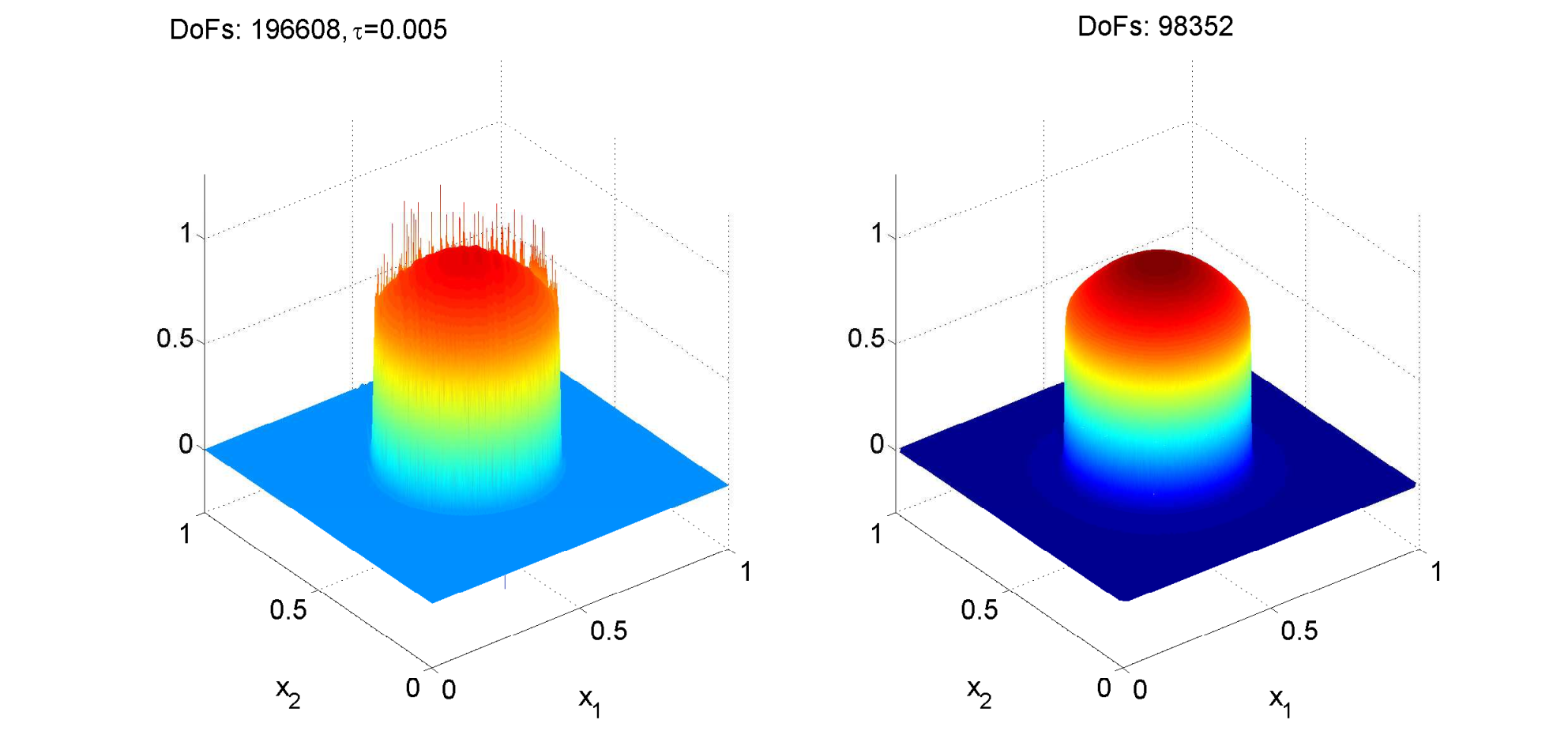
Figure 7: Example 7.1: Adaptive mesh
Refer to caption
Figure 8: Example 7.1: Uniform (left) and adaptive (right) solutions at T=0.5
()
()
Figure 9: Example 7.1: Evolution of DoFs (left) and time-steps τ\tau (right)

7.2 Coupled example with polynomial type non-linearity

The next example is a coupled non-linear problem taken from [5].

∂ui∂t−ϵ​Δ​ui+β→i⋅∇ui+u1​u2\displaystyle\frac{\partial u_{i}}{\partial t}-\epsilon\Delta u_{i}+\vec{\beta}_{i}\cdot\nabla u_{i}+u_{1}u_{2} =\displaystyle= fi,i=1,2\displaystyle f_{i},\quad i=1,2

on Ω=(0,1)2\Omega=(0,1)^{2} with the convection fields β→1=(1,0)T\vec{\beta}_{1}=(1,0)^{T} and β→2=(−1,0)T\vec{\beta}_{2}=(-1,0)^{T}, and the diffusion constant ϵ=10−5\epsilon=10^{-5}. The Dirichlet boundary conditions, initial conditions and the load functions fif_{i} are chosen so that the exact solutions are

u1​(x→,t)=12​(1−tanh⁡2​x1−0.2​t−0.85​ϵ)u_{1}(\vec{x},t)=\frac{1}{2}\left(1-\tanh\frac{2x_{1}-0.2t-0.8}{\sqrt{5\epsilon}}\right)
u2​(x→,t)=12​(1+tanh⁡2​x1+0.2​t−0.95​ϵ)u_{2}(\vec{x},t)=\frac{1}{2}\left(1+\tanh\frac{2x_{1}+0.2t-0.9}{\sqrt{5\epsilon}}\right)

We use again quadratic DG elements. We prepare an initial mesh, Fig. 11 on the left, starting with a very coarse spatial mesh and a uniform partition of the time interval [0,1][0,1] with the step-size τ=0.1\tau=0.1 until the user defined tolerances 𝐭𝐭𝐨𝐥=10−3\mathbf{ttol}=10^{-3} and 𝐬𝐭𝐨𝐥+=10−1\mathbf{stol^{+}}=10^{-1} are satisfied. Here, two sharp fronts move towards to each other and then mix directly after the time t=0.1t=0.1, Fig. 10. The movement of the fronts are also visible in Fig. 11 claiming that refinement/coarsening of the adaptive algorithm works well. We see that the sharp fronts in the cross-wind direction x2=0.5​x1+0.75x_{2}=0.5x_{1}+0.75 are almost damped out. Moreover, Fig. 11-12 show that both the spatial and temporal estimators catch the time where the two sharp fronts mix.

()
()
Figure 10: Example 7.2: Cross-section plots in the cross-wind direction at t=0.1t=0.1 (left) and t=1t=1 (right)
()
()
()
Figure 11: Example 7.2: Adaptive meshes at t=0t=0, t=0.1t=0.1 and t=1t=1 (from left to right)
()
()
Figure 12: Example 7.2: Evolution of DoFs (left) and time-steps τ\tau (right)

7.3 Non-linear ADR equation in homogeneous porous media

We consider the advection-diffusion-reaction (ADR) equation in [19] with polynomial type non-linear reaction

∂u∂t−ϵ​Δ​u+β→⋅∇u+γ​u2​(u−1)\displaystyle\frac{\partial u}{\partial t}-\epsilon\Delta u+\vec{\beta}\cdot\nabla u+\gamma u^{2}(u-1) =\displaystyle= 0in ​Ω×(0,T]\displaystyle 0\quad\text{in }\;\Omega\times(0,T]

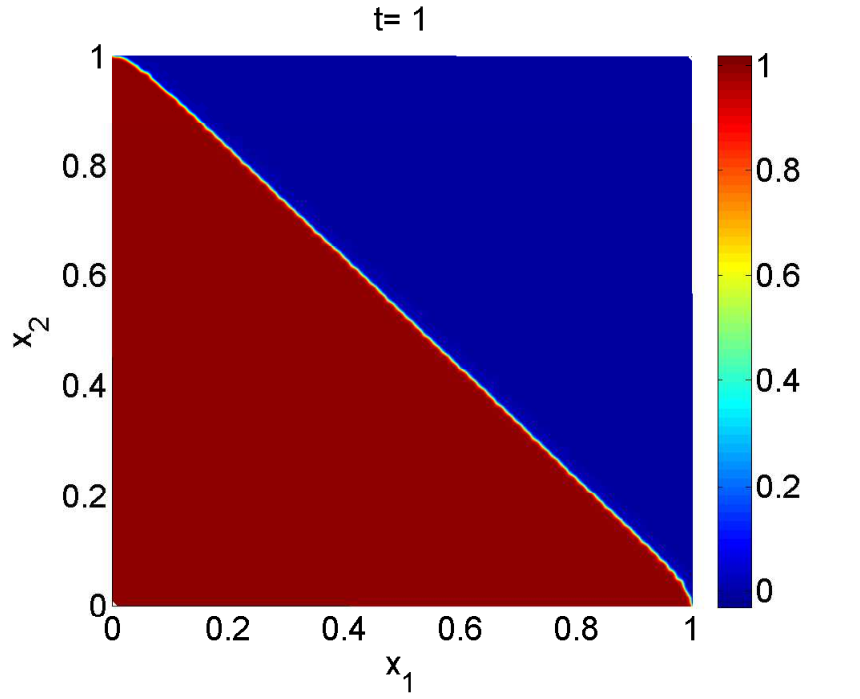
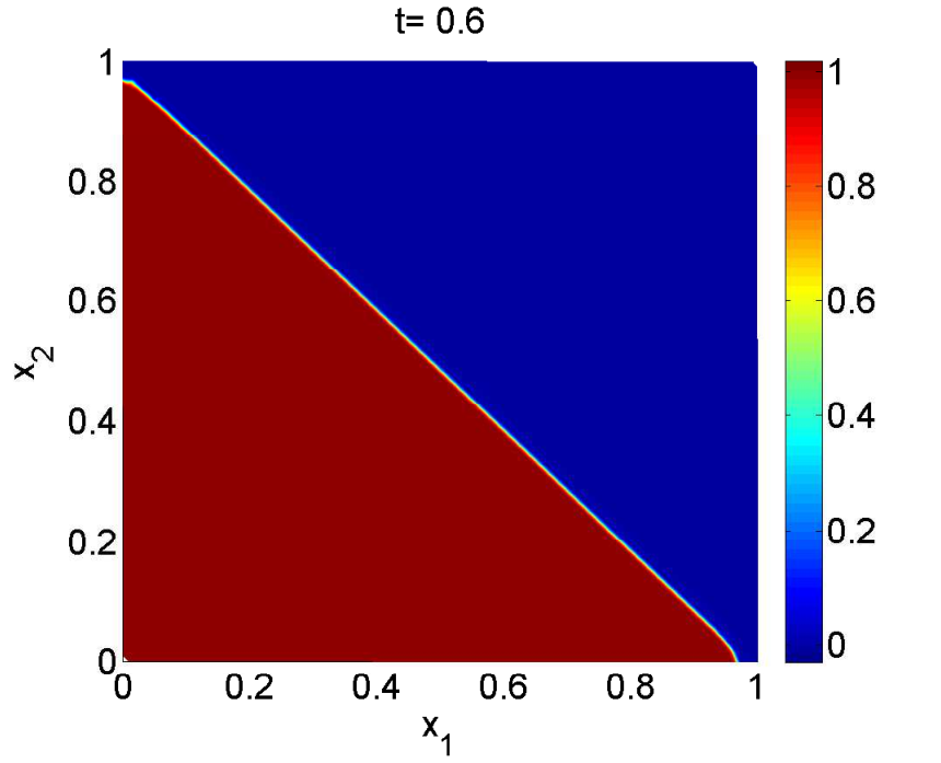
on Ω=(0,1)2\Omega=(0,1)^{2}. We take as in [19] the homogeneous dispersion tensor as ϵ=10−4\epsilon=10^{-4}, the velocity field β→=(−0.01,−0.01)T\vec{\beta}=(-0.01,-0.01)^{T} and γ=100\gamma=100. The initial and boundary conditions are chosen by the exact solution

u⁡(x→,t)=[1+exp⁡(a⁡(x1+x2−b​t)+a⁡(b−1))]−1u(\vec{x},t)=[1+\exp(a(x_{1}+x_{2}-bt)+a(b-1))]^{-1}

with a=γ/(4​ϵ)a=\sqrt{\gamma/(4\epsilon)} and b=−0.02+γ​ϵb=-0.02+\sqrt{\gamma\epsilon}. The problem is a transport of a front in homogeneous porous media. We simulate the given problem for the final time T=1T=1, and with quadratic DG elements. We begin by preparing an initial mesh starting from a very coarse spatial mesh and a uniform partition of the time interval [0,1][0,1] with the step-size τ=0.25\tau=0.25 until the user defined tolerances 𝐭𝐭𝐨𝐥=3×10⁻³\mathbf{ttol}=3\times 10^{-3} and 𝐬𝐭𝐨𝐥+=10−3\mathbf{stol^{+}}=10^{-3} are satisfied. In Fig. 13, the adaptive meshes and solution profiles are shown at the times t={0.2,0.6,1}t=\{0.2,0.6,1\} where the movement of the front can be seen. The time vs DoFs and time vs time step-size plots in Fig. 14 indicate clearly the oscillations in DoFs and time-steps due to the movement of the front.

()
()
()
Refer to caption
()
Refer to caption
()
Refer to caption
()
Figure 13: Example 7.3: Adaptive meshes (top) and solution profiles (bottom) at t=0.2t=0.2, t=0.6t=0.6 and t=1t=1 (from left to right)
()
()
Figure 14: Example 7.3: Evolution of DoFs (left) and time-steps τ\tau (right)

7.4 Non-linear ADR in deterministic heterogeneous porous media

We consider the ADR equation in [19] with Monod or Langmuir isotherm type non-linear reaction

∂u∂t−∇⋅(ϵ∇u)+β→(x)⋅∇u+u1+u\displaystyle\frac{\partial u}{\partial t}-\nabla\cdot(\epsilon\nabla u)+\vec{\beta}(x)\cdot\nabla u+\frac{u}{1+u} =\displaystyle= 0in ​Ω×(0,T]\displaystyle 0\quad\text{in }\;\Omega\times(0,T]
u⁡(x,t)\displaystyle u(x,t) =\displaystyle= 1on ​ΓD×[0,T]\displaystyle 1\quad\text{on }\;\Gamma^{D}\times[0,T]
−ϵ∇u(x,t)⋅n→\displaystyle-\epsilon\nabla u(x,t)\cdot\vec{n} =\displaystyle= 0on ​(∂Ω∖ΓD)×[0,T]\displaystyle 0\quad\text{on }\;(\partial\Omega\setminus\Gamma^{D})\times[0,T]
u⁡(x,0)\displaystyle u(x,0) =\displaystyle= 0in ​Ω\displaystyle 0\quad\text{in }\;\Omega

with Ω=(0,3)×(0,2)\Omega=(0,3)\times(0,2) and ΓD={0}×[0,2]\Gamma^{D}=\{0\}\times[0,2]. The problem represents a reaction in porous media, for instance, transport in a highly idealized fracture pattern. Here ϵ\epsilon stands for the heterogeneous dispersion tensor given by

ϵ=[10−30010−4]\epsilon=\begin{bmatrix}10^{-3}&0\\ 0&10^{-4}\end{bmatrix}

The velocity field β→​(x)\vec{\beta}(x) is determined via the Darcy’s law

β→=−k⁡(x)μ∇p\vec{\beta}=-\frac{k(x)}{\mu}\nabla p

where pp is the fluid pressure, μ\mu is the fluid viscosity and k⁡(x)k(x) is the permeability of the porous medium. Using the mass conservation property ∇⋅β→​(x)=0\nabla\cdot\vec{\beta}(x)=0 under the assumption that rock and fluids are incompressible, the velocity field β→​(x)\vec{\beta}(x) is computed by solving

∇⋅(k⁡(x)μ∇p)\displaystyle\nabla\cdot\left(\frac{k(x)}{\mu}\nabla p\right) =\displaystyle= 0in ​Ω\displaystyle 0\quad\text{in }\;\Omega
p\displaystyle p =\displaystyle= 1on ​{0}×[0,2]\displaystyle 1\quad\text{on }\;\{0\}\times[0,2]
p\displaystyle p =\displaystyle= 0on ​{3}×[0,2]\displaystyle 0\quad\text{on }\;\{3\}\times[0,2]
−k(x)∇p⋅n→\displaystyle-k(x)\nabla p\cdot\vec{n} =\displaystyle= 0on ​(0,3)×{0,2}\displaystyle 0\quad\text{on }\;(0,3)\times\{0,2\}

We simulate the given problem for the final time T=1T=1 using linear DG elements. We take the fluid viscosity μ=0.1\mu=0.1, and the permeability field as in [19] with three parallel streaks the permeability of which are 100 times greater than the permeability of the surrounding domain, see Fig. 15 on the left, by which the flow is canalized from the lower-permeability rocks into the high-permeability ones, Fig. 15 on the right. For the adaptive procedure, we prepare an initial mesh starting from a very coarse spatial mesh and a uniform partition of the time interval [0,1][0,1] with the step-size τ=0.05\tau=0.05 until the user defined tolerances 𝐭𝐭𝐨𝐥=10−3\mathbf{ttol}=10^{-3} and 𝐬𝐭𝐨𝐥+=3×10⁻⁴\mathbf{stol^{+}}=3\times 10^{-4} are satisfied. Fig. 16-17 show the adaptive meshes and concentrations at t=0.3t=0.3 and t=1t=1, where we can clearly see the flow-focusing due to the high-permeability.

()
()
Figure 15: Example 7.4: Permeability field (left) and velocity streamlines (right)
Refer to caption
Figure 16: Example 7.4: Adaptive mesh (left) and concentration (right) at t=0.3t=0.3
Refer to caption
Figure 17: Example 7.4: Adaptive mesh (left) and concentration (right) at t=1t=1

Time vs DoFs and time vs time step-size plots are given in Fig. 18. We see that initially small time steps are used and then it reaches a steady time step, Fig. 18 on the right. The number of DoFs increases (refinement dominates coarsening) monotonically after the meet of first high-permeability rock until the meet of third high-permeability rock and then the increase stops, Fig. 18 on the left. This is meaningful since there is no sharp flow canalization after the third high-permeability rock.

()
()
Figure 18: Example 7.4: Evolution of DoFs (left) and time-steps τ\tau (right)

8 Conclusion

We implemented a time-space adaptive algorithm for non-linear ADR equations based on utilizing the elliptic reconstruction technique to be able to use the elliptic a posteriori error estimator for the convection dominated parabolic problems with non-linear reaction mechanisms. We derived a posteriori error estimator in the L∞​(L2)+L2​(H1)L^{\infty}(L^{2})+L^{2}(H^{1})-type norm using backward Euler in time and SIPG in space. We demonstrated the performance of the algorithm by numerical studies.

References

  • [1] Arnold, D., Brezzi, F., Cockborn, B., Marini, L.: Unified analysis of discontinuous Galerkin methods for elliptic problems. SIAM J. Numer. Anal. 39, 1749–1779 (2002)
  • [2] Ayuso, B., Marini, L.D.: Discontinuous Galerkin methods for advection-diffusion-reaction problems. SIAM J. Numer. Anal. 47, 1391–1420 (2009)
  • [3] Bastian, P., Engwer, C., Fahlke, J., Ippisch, O.: An unfitted discontinuous Galerkin method for pore-scale simulations of solute transport. Mathematics and Computers in Simulation 81(10), 2051–2061 (2011)
  • [4] Bause, M., Schwegler, K.: Analysis of stabilized higher-order finite element approximation of nonstationary and non-linear convection-diffusion-reaction equations. Comput. Methods Appl. Mech. Engrg. 209–212, 184–196 (2012)
  • [5] Bause, M., Schwegler, K.: Higher order finite element approximation of systems of convection-diffusion-reaction equations with small diffusion. Journal of Computational and Applied Mathematics 246, 52–64 (2013)
  • [6] Bürger, R., Sepùlveda, M., Voitovich, T.: On the Proriol-Koornwinder-dubiner hierarchical orthogonal polynomial basis for the DG-FEM (2009)
  • [7] Cangiani, A., Georgoulis, E.H., Metcalfe, S.: Adaptive discontinuous Galerkin methods for nonstationary convection-diffusion problems. IMA Journal of Numerical Analysis pp. 1–20 (2013)
  • [8] Castillo, P.: Performance of discontinuous Galerkin methods for elliptic PDEs. SIAM J. Sci. Comput. 24, 524–547 (2012)
  • [9] Di Pietro, D.A., Vohralik, M.: A review of recent advances in discretization methods, a posteriori error analysis, and adaptive algorithms for numerical modeling in geosciences. Geosciences Numerical Methods 69, 701–729 (2014)
  • [10] Dobrev, V.A., Lazarov, R.D., Zikatanov, L.T.: Preconditioning of symmetric interior penalty discontinuous Galerkin FEM for elliptic problems. In: Domain Decomposition Methods in Science and Engineering XVII, Lecture Notes in Computer Science and Engineering, vol. 60, pp. 33–44. Springer (2008)
  • [11] Epshteyn, Y., Rivière, B.: Estimation of penalty parameters for symmetric interior penalty Galerkin methods. J. Comput. Appl. Math. 206, 843–872 (2007)
  • [12] Houston, P., Schwab, C., Süli, E.: Discontinuous hp-finite element methods for advection-diffusion-reaction problems. SIAM J. Numer. Anal. 39, 2133–2163 (2002)
  • [13] Klieber, W., Rivière, B.: Adaptive simulations of two-phase flow by discontinuous Galerkin methods. Computer Methods in Applied Mechanics and Engineering 196(1–3), 404–419 (2006)
  • [14] Makridakis, C., Nochetto, R.H.: Elliptic reconstruction and a posteriori error estimates for parabolic problems. SIAM J. Numer. Anal. 41(4), 1585–1594 (2003)
  • [15] Proft, J., Riviere, B.: Discontinuous Galerkin methods for convection-diffusion equations for varying and vanishing diffusivity. Int. J. Numer. Anal. Model 6(4), 533–561 (2009)
  • [16] Rivière, B.: Discontinuous Galerkin methods for solving elliptic and parabolic equations, Theory and implementation. SIAM (2008)
  • [17] Schötzau, D., Zhu, L.: A robust a-posteriori error estimator for discontinuous Galerkin methods for convection-diffusion equations. Applied Numerical Mathematics 59, 2236–2255 (2009)
  • [18] Sun, S., Wheeler, M.F.: L2(H1) norm a posteriori error estimation for discontinuous Galerkin approximations of reactive transport problems. Journal of Scientific Computing 22–23(1–3), 501–530 (2005)
  • [19] Tambue, A., Lord, G.J., Geiger, S.: An exponential integrator for advection-dominated reactive transport in heterogeneous porous media. Journal of Computational Physics 229, 3957–3969 (2010)
  • [20] Uzunca, M., Karasözen, B., Manguoğlu, M.: Adaptive discontinuous Galerkin methods for non-linear diffusion-convection-reaction equations. Computers and Chemical Engineering 68, 24–37 (2014)
  • [21] Van Slingerland, P., Vuik, C.: Fast linear solver for diffusion problems with applications to pressure computation in layered domains. Computational Geosciences pp. 1–14 (2014)