Transitionless-based shortcuts for the fast and robust generation of states
Abstract
We propose a scheme to generate states based on transitionless-based shortcuts technique in cavity quantum electrodynamics (QED) system. In light of quantum Zeno dynamics, we first effectively design a system whose effective Hamiltonian is equivalent to the counter-diabatic driving Hamiltonian constructed by transitionless quantum driving, then, realize the states’ generation within this framework. For the sake of clearness, we describe two stale schemes for states’ generation via traditional methods: the adiabatic dark-state evolution and the quantum Zeno dynamics. The comparison among these three schemes shows the shortcut scheme is closely related to the other two but better than them. That is, numerical investigation demonstrates that the shortcut scheme is faster than the adiabatic one, and more robust against operational imperfection than the Zeno one. What is more, the present scheme is also robust against decoherence caused by spontaneous emission and photon loss.
Keywords:
state; Transitionless quantum driving; Shortcuts to adiabatic passage.pacs
03.67. Pp, 03.67. Mn, 03.67. HKI Introduction
Quantum entanglement is an intriguing property of composite systems. The generation of entangled states for two or more particles is not only fundamental for demonstrating quantum nonlocality [1, 2], but also useful in quantum information processing (QIP) [3, 4]. For three-qubit entanglement, there are two main kinds of entangled states , the states [5] and the Greenberger-Horne-Zeilinger (GHZ) states [2]. These two kinds of entangled states cannot be converted to each other by local operations and classical communications. In recent years, the states attract more attentions because of its robustness against qubit loss and advantages in quantum teleportation [6]. So far, lots of theoretical schemes have been proposed to generate states in different systems via different techniques [7, 8, 9, 10, 11, 12, 13, 14]. There are two techniques famous for their robustness against decoherence in proper conditions and have been widely used in QIP: one is named stimulated Raman scattering involving adiabatic passage (STIRAP) including their variants [15, 16, 17, 18, 19], and the other one is Quantum Zeno dynamics (QZD) [20, 21, 22, 24, 23]. Generally speaking, the adiabatic passage technique is robust against variations in the experimental parameters and atomic spontaneous emission. To restrain the influence of photon leakage on the fidelity, a widely used way is choosing parameters to reduce populations of the intermediate excited states. However, such operation inevitably increase the operation time. As is known to all, using adiabatic technique (we name it “adiabatic scheme” for short in this paper) asks for an adiabatic condition that the change of a system’s Hamiltonian in time is managed to be slow to make sure each of the eigenstates of the system evolves along itself. Using QZD method, by contrast, might be faster than using adiabatic passage. But that depends, especially in multiparticle systems. Usually, in a scheme based on QZD (we name it “Zeno scheme” for short in this paper), we consider the system’s Hamiltonian as , where is the Hamiltonian of the quantum system investigated, is the coupling constant, and is viewed as an additional interaction Hamiltonian performing the measurement. When , the system’s effective Hamiltonian is approximated as , where is the th eigenvalue projection of with eigenvalue . Similar to the adiabatic passage, there is also a limited condition in a Zeno scheme that limits the system’s speed: the Zeno condition . It has been confirmed by lots of schemes that using QZD for QIP is usually robust against photon leakage but sensitive to the atomic spontaneous emission. Therefore, in order to restrain the influence of atomic spontaneous emission, some researchers introduced detunings between the atomic transitions to decrease the population of atomic excited states. That also inevitably increases the operation time. In addition, the operation time required in a scheme via QZD always needs to be controlled accurately, which increases the difficulty to realize the scheme in experiment. As we know, the operation time for a method is the shorter the better, otherwise, the method may be useless because the dissipation caused by decoherence, noise, and losses on the target state increases with the increasing of the interaction time. Many experiments also desire fast and robust theoretical methods because high repetition rates contribute to the achievement of better signal-to-noise ratios and better accuracy.
Therefore, fast and noise-resistant generation of entangled states becomes a research hotspot in recent years, especially, after the technique named “Shortcuts to adiabatic passage” (STAP) [25, 26] was proposed. This technique is related to adiabatic passage but successfully breaks the limit of the adiabatic condition. It describes a fast adiabatic-like process which is not really adiabatic but leading to the same final populations with adiabatic process. Newly, STAP has shown its charm in theory and experiment [27, 42, 28, 29, 31, 32, 30, 50, 51, 52, 53, 54, 41, 43, 44, 45, 46, 47, 48, 49, 33, 34, 35, 36, 37, 38, 39, 40, 55]. In 2014, by using transitionless tracking algorithm under large detuning condition , Lu et al. proposed an effective scheme to implement fast populations transfer and fast maximum entanglement preparation between two atoms in a cavity [30]. The idea inspires that using some traditional methods to approximate a complicated Hamiltonian into an effective and simple one first, then constructing shortcuts for the effective Hamiltonian might be a promising method to speed up a system. Soon after that, Chen et al. first combined invariant-based inverse engineering with Zeno subspaces to construct shortcuts to perform fast and noise-resistant populations transfer for multiparticle systems [29]. In their method, they demonstrated that besides constructing STAP, slightly broking down the Zeno condition under certain conditions is another simple way to speed up the evolution. Soon after that, similar ideas with slightly breaking the Zeno condition down are rapidly used to perform fast and noise-resistant QIP [32, 33, 57, 58, 56].
Motivated by the above analysis, we discuss how to construct STAP to rapidly generate states by using the approach of “transitionless tracking algorithm” in cavity QED systems. Different from ref. [32] which proposed a method through combining Lewis-Riesenfeld theory and Zeno subspaces to generate a -atom state by atoms, we do not need to abandon any atoms. An -atom is fast generated directly by atoms in one step. In order to explain the charm by using STAP to generate states, we first give a brief description about generation of states via two traditional methods (STIRAP and QZD). Then, we propose the scheme by using transitionless tracking algorithm in detail. The comparison among these three schemes demonstrates that the shortcut scheme is not only faster than the adiabatic one, and more robust against operational imperfection than the Zeno one. What is more, this method might be promising when it comes to generation of multi-level and multi-qubit entangled states, i.e., the singlet states.
The rest of the paper is organized as follows. In section II, we give the model of atom-cavity system and introduce two schemes to generate states via traditional adiabatic method and Zeno method. Then in section III, we use the transitionless-based shortcuts method to propose a fast and noise-resistant scheme to generate states. The conclusion is derived in section IV.

II theoretical Generation of states in a three-atom system
For simplicity, we assume that three -type atoms (, , ) are trapped in a cavity () as shown in Figs. 1 (a) and (b), each atom has an excited state and two ground states and . Atomic transition is resonantly driven by classical field , and the transition is coupled resonantly to the cavity with coupling . Under the rotating-wave approximation (RWA), the interaction Hamiltonian for this system reads
| (1) |
where is the annihilation operator of the cavity. We assume the initial state of the system is , the system will evolve within a single-excitation subspace spanned by:
| (2) | |||||
| (3) | |||||
| (4) | |||||
| (5) | |||||
| (6) | |||||
| (7) | |||||
| (8) |
Here it is worth noting that in a natural case, the atoms are usually in the same state initially, i.e., the steady state . So, it is necessary to prepare the initial state before implementing the scheme. That is, a population transfer is imperative before the scheme. Fortunately, such operation is not hard to be realized. pulse, stimulated Raman adiabatic passage, large detuning dynamics, and many other techniques are applicable to transfer population from to . Therefore, in subspace , the interaction Hamiltonian is simplified as (we set to be constant coupling coefficients)
| (9) | |||||
| (10) | |||||
| (11) |
For the sake of clearness, we will describe two traditional different methods (STIRAP and QZD) to generate states in brief.


II.1 Based on STIRAP
For the Hamiltonian in eq. (9) in the single-excitation subspace, we easily find a dark state
| (12) |
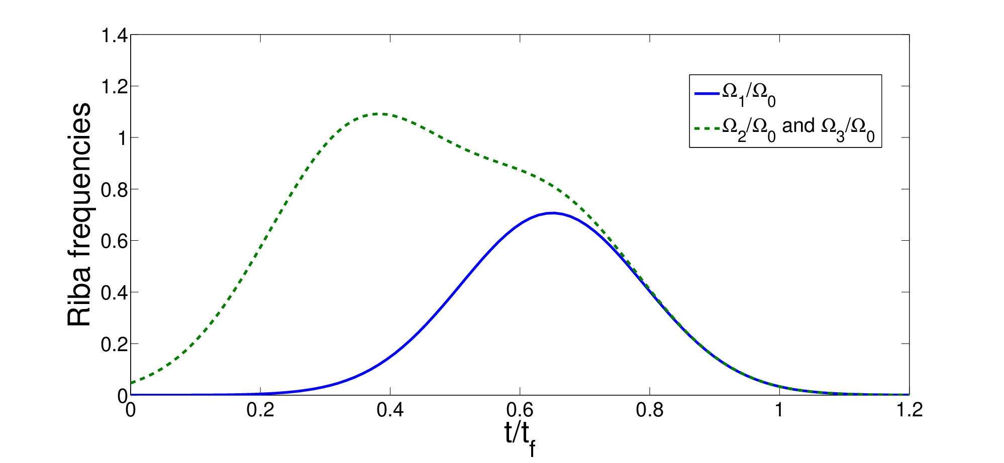
where is the normalization coefficient. If we choose at first and make sure that the adiabatic condition is satisfied, where is the th eigenstate with nonzero eigenvalue , the initial state will follow closely. Then, we slowly decrease and while increase until at time . Accordingly, the dark state becomes which is the state. As shown in Fig. 3, to complete this process, we choose the Rabi frequencies as (we set )
| (13) | |||||
| (17) | |||||
where is the amplitude and are related parameters. To meet the conditions mentioned above, we choose , , and . Generally speaking, the adiabatic condition is satisfied better with a relatively large because the nonzero eigenvalue is proportional to . Fig. 3 shows the fidelity of the state in adiabatic scheme versus the interaction time and . The fidelity for any target state is given through the relation , where is the density operator given through . As shown in Fig. 3, the fidelity is getting higher with both the increases of and . It seems that when , a high-fidelity state is achievable. That means when is large enough, we also can create a state in a short interaction time via adiabatic passage. But further investigation tells us that the system’s evolution is far different from adiabatic dark-state evolution with a relatively large and a short interaction time . Fig. 4 (a) shows the time-dependent populations for states {, , , } when and , Fig. 4 (b) shows the time-dependent populations for states {, , , } when and , and Fig. 4 (c) shows time-dependent evolution of the dark state . The comparison of these three figures draws a result that even with a large , a relatively long interaction time is still necessary to make sure the controlling parameters change slowly enough to allow adiabatic passage from an initial state to a target state. In addition, because a relatively large might cause that the RWA is no longer effective for the system, and it also means a great population of state including a cavity-excited state that makes the system sensitive to the cavity photon leakage, it is better to choose a relatively small and a long interaction time for an adiabatic process.

II.2 Based on QZD
Before we start using QZD to create a three-atom state, we set and use two orthogonal vectors and to rewrite the Hamiltonian in eq. (9) as
| (20) | |||||
| (22) |
It is obvious that when the initial state is , the terms containing are negligible because they are decoupled to the time evolution of initial state. Then, under the condition (Zeno condition), the subspace is split into three Zeno subspaces according to the degeneracy of eigenvalues of ,
| (23) | |||||
| (24) |
where
| (25) | |||||
| (26) | |||||
| (27) |
corresponding eigenvalues , , and . Under the Zeno condition, we obtain the effective Hamiltonian governing the evolution
| (28) |
where . When and are constant parameters, the general evolution of eq. (9) by solving the Schrödinger equation in time is
| (31) | |||||
where . By choosing and , the final state becomes which is the state.
In general, the interaction time required in a Zeno scheme is shorter than that in an adiabatic scheme. For example, in the present scheme, when we choose relatively large laser pulses, i.e., , the interaction time in the Zeno scheme is only about . However, it is well known that the interaction time should be controlled accurately in a scheme via QZD. We plot the fidelity of the state in Zeno scheme versus the variation in in Fig. 5. Here we define as the deviation of any parameter , where is the actual value and is the ideal value. It is clear that a deviation causes a reduction about in the fidelity, which shows the scheme is sensitive to the variation of the interaction time. In experiment, if we choose a related parameter GHZ, the required interaction time is s. That means, the experimental researchers should accurately control the interaction time to ensure the deviation in is less than s. That is really a challenge in the current experimental technology. Moreover, known from eq. (31), the intermediate state including atomic-excited states would be greatly populated during the evolution if is too large, and that might make the system sensitive to the spontaneous emission.

III Using STAP to fast generate a state
Different from the two methods (adiabatic scheme and Zeno scheme) mentioned above, we start from finding a Hamiltonian which is related to to fast generate a state via STAP. The key point to construct shortcuts for a system governed by is to find out a Hamiltonian which drives the instantaneous eigenstates () of exactly. Known from Berry’s general transitionless tracking algorithm [59], the Hamiltonian can be reverse engineered from . And disregarding the effect of phases, the simplest Hamiltonian is derived in form of
| (32) |
However, it seems impossible to directly design such Hamiltonian from according to eq. (9) because the eigenstates given by solving the intrinsic equation are very complex such that mathematically solving eq. (32) seems an outstanding challenge. So here we make a limiting condition to simplify the calculation. Under this condition, by substituting the instantaneous eigenstates of in eq. (9) into eq. (32), we obtain the Hamiltonian that exactly drives the eigenstates of
| (33) | |||||
| (35) |
where , , and . Obviously, there is no way to directly apply a pulse between the state and . So, to realize such a Hamiltonian, we need to find out an alternative physically feasible (APF) system whose effective Hamiltonian is equivalent to . The model of the APF system is the same as that in Fig. 1 (a). The difference happens in the atomic level configuration as shown in Fig. 1 (c), each atom also has three levels , , and . The transition is non-resonantly driven by classical field with time-dependent Rabi frequency and detuning . The transition is coupled non-resonantly to the cavity with coupling and detuning . Similar to the transformation from eq. (9) to eq. (20), the interaction Hamiltonian in the subspace (the single-excitation subspace for this model is also spanned by eq. (2)) for the present model can be described as (we set and )
| (36) | |||||
| (40) | |||||
| (42) | |||||
| (44) |
The terms including are also neglected because they are decoupled to the time evolution of initial state when the initial state is set as . Using the eigenstates of to rewrite this Hamiltonian and performing the unitary transformation , we obtain
| (47) | |||||
| (49) |
Consider , we neglect terms containing high oscillating frequencies and terms decoupled to the time evolution of initial state. Then we obtain an effective Hamiltonian
| (52) | |||||
Then by adiabatically eliminating the state under large detuning condition , we obtain an effective Hamiltonian
| (55) | |||||
When we choose and (here is a real number),
| (56) | |||||
| (57) |
where . It is not hard to find, the first term in eq. (56) only affects the global phase for the dynamics governed by . So, in fact, we can directly take off the first term and further simplify the Hamiltonian as when we pay no attention to the global phase. That means, as long as and ; the Hamiltonian for speeding up the adiabatic dark-state evolution governed by under condition has been constructed. As we mentioned above, to create a three-atom state by adiabatic dark-state evolution, the Riba frequencies and can be chosen in the form in eq. (13). Hence, is given
| (58) |
If we set , according to eq. (13) we can obtain two dimensionless parameters
| (59) | |||||
| (61) |
Therefore, putting eqs. (23) and (59) into eq. (58), we obtain
| (62) |
where
| (63) |
is a dimensionless wave function. A brief analysis of tells us that the amplitude of is close to . That is, the amplitude of is mainly dominated by . According to the limited conditions above, we have
| (64) | |||||
| (66) |
When is a constant value, under the premise that the interaction time is short, to meet the first condition in eq. (64), it is better to choose a smaller , while to meet the second condition, a larger is required. This is also demonstrated in Fig. 6 which shows the fidelity of the state in the shortcut scheme versus parameters and . We can find, too small or too large cause a long operation time for the scheme. Then, we choose a set of suitable parameters {} for the scheme. As shown in Fig. 7 (a), with these parameters, we can achieve a perfect populations transfer after very slightly correcting a related parameter () by numerical simulation. The parameter should be slightly corrected because speeding up the evolution needs to slightly broke the Zeno condition, and that cause a slight failure of the approximation. We plot the time evolution of the populations in intermediate states and in Fig. 7 (b) to prove this operation is necessary. In the figure, the state should have been neglected is slightly populated (the Zeno condition is slightly broken) while the state is negligible (the second condition in eq. (64) is fulfilled). We give a comparison of the fidelities via these three different methods in Fig. 7 (c). Contrasting with the Zeno method, the advantage of the present shortcut method is obvious: the shortcut scheme is more robust against operational imperfection than the Zeno one, especially, it is not necessary to control the interaction time accurately. As demonstrated in Fig. 8, the fidelity almost keeps unchanging with the variation , where is the total operation time chosen to complete the scheme, and a deviation which means the variation in the amplitude of only causes a reduction about 1% in the fidelity.


Now, we will check the robustness of the shortcut scheme against possible mechanisms of decoherence. The evolution of the system can be modeled by a master equation in Lindblad form when the decoherence is considered,
| (67) |
where is the density operator for the whole system and are the Lindblad operators. For the shortcut scheme, there are seven lindblad operators governing the dissipation:
| (68) | |||||
| (69) | |||||
| (70) | |||||
| (71) |
where () are the atomic spontaneous emissions and is the cavity decay. We set for simplicity. Then by numerically solving the master equation in eq. (68), we plot the fidelity of the state in the shortcut scheme versus and in Fig. 9 (a). We can find that the shortcut scheme is more sensitive to the cavity decay than atomic spontaneous emissions with parameters {}. The reason has been mentioned above that with this set of parameters, the Zeno condition is not satisfied faultlessly. So the states and containing cavity-excited state are populated in a certain extent during the evolution. Furthermore, the parameters can be selected properly to restrain the cavity decay in the experiment according to eq. (64). For example, when we choose {, }, the Zeno condition can be satisfied well. We plot Fig. 9 (b) depicting the fidelity of the state governed by the APF Hamiltonian versus and when {, }. It shows that the influence of cavity decay is restrained with these parameters. However, it is without doubt that the scheme is robust because the fidelity decreases slowly and even when , we still can create a state with a high fidelity .
This scheme can be easily generalized to generate -atom states. We assume -type atoms are trapped in a cavity. For the original Hamiltonian, the atomic level configuration of each atom is the same as that in Fig. 1 (a), and for the APF Hamiltonian, the atomic level configuration of each atom is the same as that in Fig. 1 (c). Suppose that the atoms ‘see’ the same field, and spatial separation size of these atoms is much bigger than the wavelength of the emitted radiation, so the atomic dipole-dipole interaction can be omitted. In this case, the interaction Hamiltonian for the original Hamiltonian reads
| (72) |
and the APF Hamiltonian reads
| (73) |
We consider that the initial state of the system is in . For the atom , the classical field drives the transition resonantly between the level and with the Rabi frequency . Then, atom will emit a photon which will be absorbed by one of the other atoms with the same probability when . Therefore, the excited process of atoms (in this part, the “ atoms” means the atoms except the atom ) can be described by the state . Then, by setting , the classical fields will drive the state to . Hence, the single-excitation subspace could be spanned by
| (74) | |||||
| (75) | |||||
| (76) | |||||
| (77) | |||||
| (78) |
Meanwhile, the Hamiltonian in the single-excitation subspace can be written as
| (79) |
Similarly, the APF Hamiltonian in the single-excitation subspace is
| (82) | |||||
Obviously, the Hamiltonians in eqs. (79) and (82) are in the same form with those in eqs. (20) and (36), respectively. Therefore, similar as above, under the condition and , where are the nonzero eigenvalues of , and will be approximated as and , respectively. By setting and , the effective Hamiltonian which is equivalent to the counter-diabatic driving Hamiltonian of the original Hamiltonian will be achieved. Then, the shortcut can be constructed and the -qubit states can be rapidly generated.
In a real experiment, the cesium atoms which have been cooled and trapped in a small optical cavity in the strong-coupling regime [60, 61] can be used in this scheme. On the other hand, a set of cavity QED parameters MHz is predicted to be available in an optical cavity [62]. With these parameters, the fidelity of the state in the shortcut scheme is .


IV conclusion
In this paper, we have proposed a scheme to fast generate states via transitionless-based shortcuts. In order to highlight the advantages of the present scheme, we have described two similar schemes based on STIRAP and QZD. The comparison among these three schemes demonstrates that the shortcut scheme is faster than the adiabatic one, and more robust against operational imperfection than the Zeno one. Numerical investigation also demonstrates the present scheme is robust against the decoherence caused by both atomic spontaneous emission and photon leakage. When it comes to the generation of -atom states, the only change is setting and . Known from ref. [63], the Hamiltonian for a system with three four-level atoms trapped in a cavity also can be approximated into an effective Hamiltonian in form of eq. (28). For a similar model described in ref. [64], if the atomic transitions are non-resonant, one can also obtain an effective Hamiltonian in form of eq. (55). That means, with the same method in section III, a multi-qubit singlet state also can be fast generated. In addition, the shortcut method might also show its glamour in other fields, for example, fast transfer of entanglement [32, 65] That demonstrates the present method has a wide rang of application in quantum information processing. This might lead to a useful step toward realizing fast and noise-resistant quantum information processing for multi-qubit systems in current technology.
V Acknowledgments
This work was supported by the National Natural Science Foundation of China under Grants No. 11575045 and No. 11374054, the Foundation of Ministry of Education of China under Grant No. 212085, and the Major State Basic Research Development Program of China under Grant No. 2012CB921601.
References
- [1] J. S. Bell, Physics (Lon Island City, NY) 1, 195 (1965).
- [2] D. M. Greenberger, M. A. Horne, A. Shimony, and A. Zeilinger, Am. J. Phys. 58, 1131 (1990).
- [3] A. K. Ekert, Phys. Rev. Lett. 67, 661 (1991).
- [4] N. Gisin and S. Massar, Phys. Rev. Lett. 79, 2153 (1997).
- [5] W. Dür, G. Vidal, and J. I. Cirac, Phys. Rev. A 62, 062314 (2000).
- [6] C. H. Bennett, G. Brassard, C. Crepeau, R. Jozsa, A. Peres, and W. K. Wootters, Phys. Rev. Lett. 70, 1895 (1993).
- [7] N. B. An, Phys. Lett. A 344, 77 (2005).
- [8] S. B. Zheng, J. Opt. B 7, 10 (2005).
- [9] J. Song, Y. Xia, and H. S. Song, J. Phys. B 40, 4503 (2007).
- [10] T. Bastin, C. Thiel, J. von Zanthier, L. Lamata, E. Solano, and G. S. Agarwal, Phys. Rev. Lett. 102, 053601 (2009).
- [11] X. W. Wang, G. J. Yang, Y. H. Su, and M. Xie, Quant. Info. Proc. 8, 431 (2009).
- [12] R. X. Chen and L. T. Shen, Phys. Lett. A 375, 3840 (2011).
- [13] M. Lu, Y. Xia, J. Song, and N. B. An, J. Opt. Soc. Am. B 30, 2142 (2013).
- [14] Y. H. Chen, Y. Xia, and J. Song, Quant. Info. Proc. 12, 3771 (2013).
- [15] M. P. Fewell, B. W. Shore, and K. Bergmann, Aust. J. Phys. 50, 281 (1997).
- [16] K. Bergmann, H. Theuer, and B. W. Shore, Rev. Mod. Phys. 70, 1003 (1998).
- [17] N. V. Vitanov, T. Halfmann, B. W. Shore, and K. Bergmann, Annu. Rev. Phys. Chem. 52, 763 (2001).
- [18] P. Král, I. Thanopulos, and M. Shapiro, Rev. Mod. Phys. 79, 53 (2007).
- [19] L. B. Chen and W. Yang, Laser Phys. Lett. 11, 105201 (2014).
- [20] B. Misra and E. C. G. Sudarshan, J. Math. Phys. 18, 756 (1977).
- [21] W. M. Itano, D. J. Heinzen, J. J. Bollinger, and D. J. Wineland, Phys. Rev. A 41, 2295 (1990).
- [22] P. Kwiat, H. Weinfurter, T. Herzog, A. Zeilinger, and M. A. Kasevich, Phys. Rev. Lett. 74, 4763 (1995).
- [23] P. Facchi, V. Gorini, G. Marmo, S. Pascazio, and E. C. G. Sudarshan, Phys. Lett. A 275, 12 (2000).
- [24] P. Facchi and S. Pascazio, Phys. Rev. Lett. 89, 080401 (2002).
- [25] X. Chen, I. Lizuain, A. Ruschhaupt, D. Guéry-Odelin, and J. G. Muga, Phys. Rev. Lett. 105, 123003 (2010).
- [26] E. Torrontegui, S. Ibáñez, S. Martínez-Garaot, M. Modugno, A. del Campo, D. Gué-Odelin, A. Ruschhaupt, X. Chen, and J. G. Muga, Adv. Atom. Mol. Opt. Phys. 62, 117 (2013).
- [27] A. del Campo, Phys. Rev. Lett. 111, 100502 (2013).
- [28] S. Masuda and K. Nakamura, Phys. Rev. A 84, 043434 (2011).
- [29] Y. H. Chen, Y. Xia, Q. Q. Chen, and J. Song, Phys. Rev. A 89, 033856 (2014).
- [30] M. Lu, Y. Xia, L. T. Shen, J. Song, and N. B. An, Phys. Rev. A 89, 012326 (2014).
- [31] M. Lu, Y. Xia, L. T. Shen, and J. Song, Laser Phys. 24, 105201 (2014).
- [32] Y. H. Chen, Y, Xia, Q. Q. Chen, and J. Song, Laser Phys. Lett. 11, 115201 (2014); Phys. Rev. A 91, 012325 (2015).
- [33] Y. H. Chen, Y, Xia, J. Song, and Q. Q. Chen, Sci. Rep 5, 15616 (2015).
- [34] S. Ibáñez, X. Chen, E. Torrontegui, J. G. Muga, and A. Ruschhaupt, Phys. Rev. Lett. 109, 100403 (2012).
- [35] S. Martínez-Garaot, E. Torrontegui, X. Chen, and J. G. Muga, Phys. Rev. A 89, 053408 (2014).
- [36] T. Opatrný and K. Mølmer, New J. Phys. 16, 015025 (2014).
- [37] H. Saberi, T. Opatrny, K. Mølmer, and A. del Campo, Phys. Rev. A 90, 060301(R) (2014).
- [38] S. Ibáñez, X. Chen, and J. G. Muga, Phys. Rev. A 87, 043402 (2013).
- [39] E. Torrontegui, S. Martínez-Garaot, and J. G. Muga, Phys. Rev. A 89, 043408 (2014).
- [40] B. T. Torosov, G. D. Valle, and S. Longhi, Phys. Rev. A 87, 052502 (2013); 89, 063412 (2014).
- [41] J. G. Muga, X. Chen, A. Ruschhaup, and D. Guéry-Odelin, J. Phys. B 42, 241001 (2009).
- [42] X. Chen, A. Ruschhaupt, S. Schmidt, A. del Campo, D. Guéry-Odelin, and J. G. Muga, Phys. Rev. Lett. 104, 063002 (2010).
- [43] X. Chen and J. G. Muga, Phys. Rev. A 82, 053403 (2010).
- [44] J. F. Schaff, P. Capuzzi, G. Labeyrie, and P. Vignolo, New J. Phys. 13, 113017 (2011).
- [45] E. Torrontegui, S. Ibáñez, X. Chen, A. Ruschhaupt, D. Guéry-Odelin, and J. G. Muga, Phys. Rev. A 83, 013415 (2011).
- [46] X. Chen, E. Torrontegui, D. Stefanatos, J. S. Li, and J. G. Muga, Phys. Rev. A 84, 043415 (2011).
- [47] E. Torrontegui, X. Chen, M. Modugno, S. Schmidt, A. Ruschhaupt, and J. G. Muga, New J. Phys. 14, 013031 (2012).
- [48] Y. Li, L. A. Wu, and Z. D. Wang, Phys. Rev. A 83, 043804 (2011).
- [49] A. del Campo, Phys. Rev. A 84, 031606(R) (2011); Eur. Phys. Lett. 96, 60005 (2011).
- [50] A. Ruschhaupt, X. Chen, D. Alonso, and J. G. Muga, New J. Phys. 14, 093040 (2012).
- [51] J. F. Schaff, X. L. Song, P. Vignolo, and G. Labeyrie, Phys. Rev. A 82, 033430 (2010).
- [52] J. F. Schaff, X. L. Song, P. Capuzzi, P. Vignolo, and G. Labeyrie, Eur. Phys. Lett. 93, 23001 (2011).
- [53] A. Walther, F. Ziesel, T. Ruster, S. T. Dawkins, K. Ott, M. Hettrich, K. Singer, F. Schmidt-Kaler, and U. Poschinger, Phys. Rev. Lett. 109, 050502 (2012).
- [54] S. Y. Tseng and X. Chen, Opt. Lett. 37, 5118 (2012).
- [55] X. Chen, E. Torrontegui, and J. G. Muga, Phys. Rev. A 83, 062116 (2011).
- [56] L. C. Song, Y. Xia, and J. Song, J. Mod. Opt. 61, 1290 (2014).
- [57] Y. Liang, S. L. Su, Q. C. Wu, X. Ji, and S. Zhang, Opt. Exp. 23, 005064 (2015).
- [58] Y. Liang, Q. C. Wu, S. L. Su, and S. Zhang, Phys. Rev. A 91, 032304 (2014).
- [59] M. B. Berry, J. Phys. A 42, 365303 (2009).
- [60] J. Ye, D. M. Vernooy, and H. J. Kimble, Phys. Rev. Lett. 83, 4987 (1999).
- [61] J. McKeever, J. R. Buck, A. D. Boozer, A. Kuzmich, H. C. N agerl, D. M. Stamper-Kurn, and H. J. Kimble, Phys. Rev. Lett. 90, 133602 (2003).
- [62] S. M. Spillane, T. J. Kippenberg, K. J. Vahala, K. W. Goh, E. Wilcut, and H. J. Kimble, Phys. Rev. A 71, 013817 (2005).
- [63] X. Q. Shao, H. F. Wang, L. Chen, S. Zhang, Y. F. Zhao, and K. H. Yeon, New J. Phys. 12, 023040 (2010).
- [64] Z. C. Shi, Y. Xia, J. Song, and H. S. Song, Quant. Info. Proc. 12, 411 (2013).
- [65] T. Qiu and G. J. Yang, Phys. Rev. A 89, 052312 (2014).