Discontinuous Piecewise Polynomial Neural Networks
Abstract
An artificial neural network is presented based on the idea of connections between units that are only active for a specific range of input values and zero outside that range (and so are not evaluated outside the active range). The connection function is represented by a polynomial with compact support. The finite range of activation allows for great activation sparsity in the network and means that theoretically you are able to add computational power to the network without increasing the computational time required to evaluate the network for a given input. The polynomial order ranges from first to fifth order. Unit dropout is used for regularization and a parameter free weight update is used. Better performance is obtained by moving from piecewise linear connections to piecewise quadratic, even better performance can be obtained by moving to higher order polynomials. The algorithm is tested on the MAGIC Gamma ray data set as well as the MNIST data set.
Keywords:
artificial neural network , piecewise polynomial , discontinuous , high order , autoencoder , FLANN1 Introduction
Neural networks and their application to deep learning have become a focus of research due to the success of the algorithms on several types of problems [23, 2, 11]. The goal of this work is to create a multi-layer artificial neural network where connections between units are active only in a finite range. This naturally leads to grouping connections together into functional links that span the full range of input values. Each connection then is called a sub link of the complete link. Each sub link is represented using piecewise polynomial with compact support. The resulting link looks like a one dimensional grid of discontinuous piecewise polynomials.
The motivation for this work comes from the (1) the knowledge that activation of functional elements in biological neural networks is extremely sparse; (2) the idea that fewer layers in deep neural networks are required if one increases the computational capability of each layer; (3) the fact that the use of piecewise quadratic or higher order polynomials in an ANN results in increased polynomial output whereas the output of a piecewise linear network remains piecewise linear regardless of the number of layers; (4) increasing the sparsity (adding additional sub links) can theoretically increases computational power without increasing computational time; (5) higher order approximations are known to reduce the problem of adversarial examples [5] and (6) it has been shown that dendrites (dendritic spines) are not just passive elements, but perform computations themselves [33].
The algorithm starts with a simple technique for approximating functions, using piecewise discontinuous polynomials. Typically, discontinuous functions are avoided in artificial neural networks because gradient descent derivatives are not defined at the discontinuities. In this paper, gradient descent is used as we wait for a alternate algorithms to be developed, one possible approach is recursive decomposition as described by Friesen in [8]. The discontinuities act to break up the network into a series of sub networks. Gradient descent is applied to each of these sub networks separately and good results are achieved. The fact that this works is not entirely surprising given that the dropout technique [12, 32] has the same effect on a network during training and is equivalent to training on a discontinuous network. To see this, evaluate a network with half the hidden neurons dropped out and record the result. Then select another set of random neurons to drop out and again evaluate the network with the same input. The output from the two cases will be different and so the network is discontinuous during training as a result of dropout. Note that at least one discontinuity per link should be used to remain a universal approximator as described by [20]. The discontinuous network tends to produce over fitted results in many problems. Over-fitting is resolved by using the dropout regularization technique described by [12, 32]. In addition, a parameter free weight update method as described by [30] is used to reduce the parameter search space. Lagrange polynomials are used to describe the piecewise polynomial functions and, as such, the weights of the polynomial are the actual value of the polynomial at specific locations.
In this paper, the link is the important computational element, but this approach can just as well be applied to the unit. Piecewise polynomial approaches have been investigated in the CMAC architecture [16] and more recently the rectified linear unit [24], has become a popular activation function which is piecewise linear . High order neural network using higher order weighting terms are described by several authors including [10, 31, 13, 6, 4] and functional link artificial neural networks (FLANN) by [25, 26, 28], which is the approach used in this paper. Discontinuous neural networks have been discussed in many articles, especially with respect to recurrent neural network including [7, 22, 9] focused on convergence state estimation and stability and by [35] where a unique recurrent high order algorithm is derived for financial modeling, but where additional free parameters (weights) are added to the unit and a few simulations are performed with piecewise high order elements. There is very little work on multi-layer high order discontinuous polynomial networks. In this paper the algorithm is tested by performing simple curve fitting through the sine wave using a single link, and then classification with the MAGIC gamma ray detection data set and the MNIST data set. The MNIST test is performed using multiple autoencoders. The unique contribution of this paper is the application and development of novel algorithm, using discontinuous piecewise polynomial approximation, in a multi-layer neural network as well as the use of the parameter free weight update described by [30]. The algorithm opens the possibility of using a variety of complicated, discontinuous elements in an artificial neural network using back propagation.
Section 2 describes the algorithm used in this paper including backpropagation with discontinuities, weight initialization and link input range selection. In Section 3 we demonstrate the algorithm on 3 problems: a simple 1D function approximation; the Magic gamma ray data set; the MNIST data set. In Section 4 we conclude the paper.
2 Algorithm
Definitions used in this paper are defined in table 1.
| Link | Is the connection between two units. |
|---|---|
| Sub Link | A link is split into sub links. |
| The weight of a sub link. | |
| the weight of the link. | |
| The basis function of a sub link. | |
| The number of active links into a unit. | |
| The number of active links out of a unit. | |
| The number of Chebyshev-Lobatto nodes. | |
| The input to the link. | |
| The Chebyshev-Lobatto node. | |
| The measured output value for output link | |
| The desired output value for output link | |
| The output function for link . | |
| The output for link . | |
| The network error for a single input. | |
| Time to completion using sub links with nodes |
There are two natural ways to apply higher order approximations in artificial neural networks. The first is to replace the single weight at the link with multiple adjustable weights describing a more complicated link function - this is a functional link neural network (FLANN) as described by [25] and demonstrated by [27]. The alternative is to add adjustable parameters to the unit that describe a changing activation function, in this case adjustable parameters exist in both the unit and the link. In this paper we chose the FLANN approach as it can be written slightly more compactly while maintaining weights defined at the link.
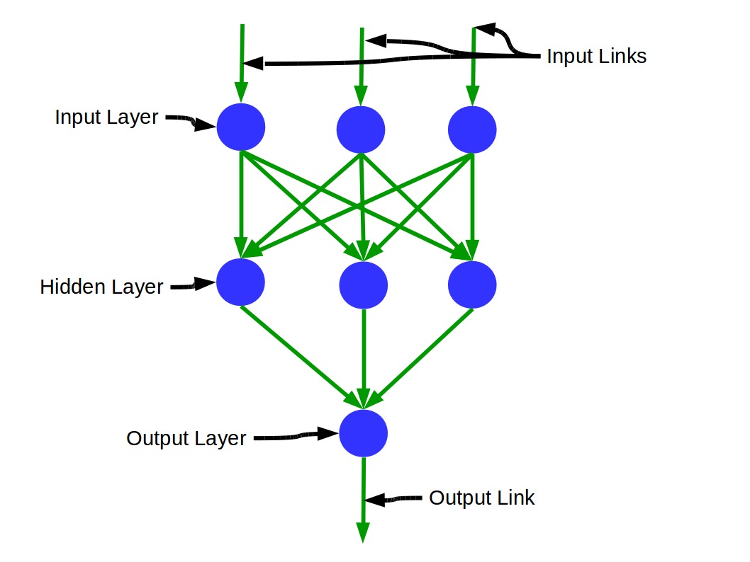
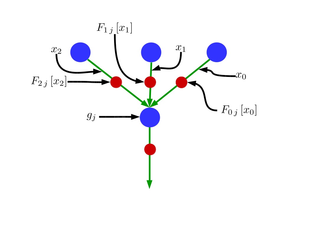
The error correction algorithm used is backpropagation as described by [29] applied to a FLANN with a minor modification described in Section 2.1. The weight update rule is defined by using the parameter free weight update rule described by [30]. A slight modification to this rule is that the maximum learning rate is set to 0.9. The network description is that of a standard feed forward network, see Figure 1, with input links and output links added. Labels for a network element are shown in figure 2. The main differences of the algorithm compared to a standard network [29] are: (1) there are multiple weights per link; (2) No bias units are used; (3) the unit averages the input signal to produce an output instead of applying a more complex activation function; (4) input/output links are added which can be used to normalize and shift the data to the desired input/output range.
The weight function of a sub link is described by the following equation,
| (1) |
with the basis functions given by the Lagrange polynomials
The Lagrange polynomial is useful because it has the value at and has the value 0 at all other . The interpolation nodes are given by the Chebyshev-Lobatto nodes, these differ from pure Chebyshev nodes in that the end points of the domain are included. The Chebyshev-Lobatto nodes are given by,
where ranges from to and is the total number of Chebyshev-Lobatto points. This means that in Equation (1) the value of the function at is . Using this approach we can easily limit the range of a polynomial interpolation by limiting the range of the weights . For clarity we provide the polynomials for both a linear and quadratic interpolation. In the linear case (assuming and )
In the quadratic case we assume , , the basis functions are
In addition to the high order weighting, discontinuities are used along with the piecewise polynomial approximation. This means that the function is different depending on the range of the input variable . In particular we have the definition
| (2) |
At the unit, the average of the incoming signals is computed. The unit could be a sigmoid, but it is not needed since the non-linearity is provided by the presence of at least one discontinuity, so only a simple average is used as the activation function of the unit.
The averaging is important because the function only has a valid solution in a finite range so it is important to guarantee that any signal passed to is within that range. This can easily be accomplished by choosing initial and correctly. is the number of input signals (not the total number of input sub links).
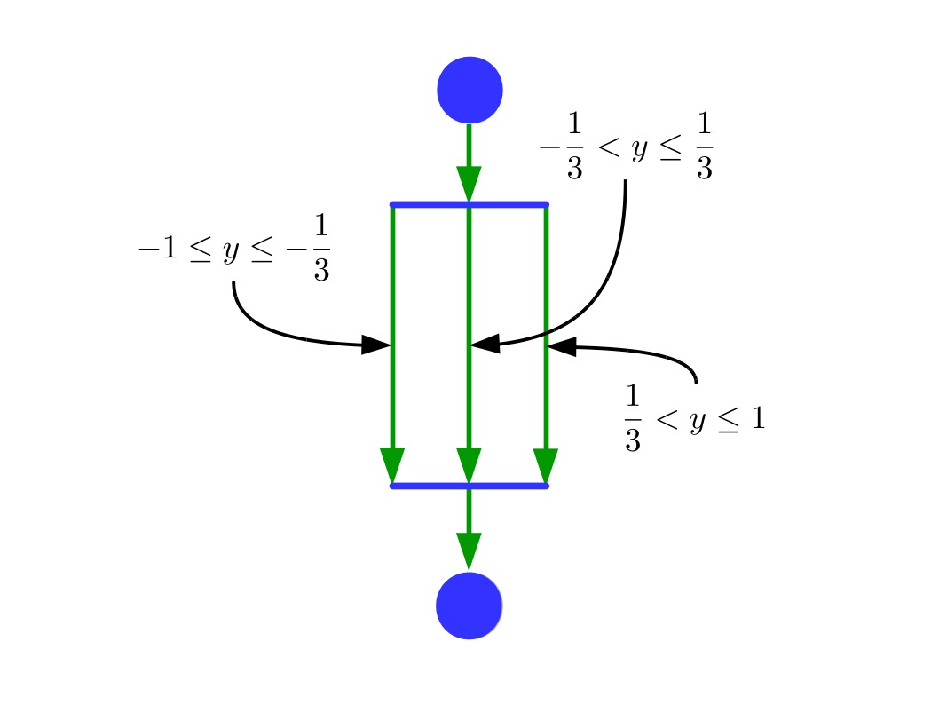
The idea to use a discontinuous piecewise polynomial comes from a pair of units with multiple links between the units, see Fig. 3. Only a single link is active depending on the output value of the unit. Equation (2) can be described as a set of links between two units where only one link passes an output signal for a given input signal. As a result, the links are grouped together in a bundle (Equation 2) and shown in figure 4. The standard link of a neural network described in this paper then consists of one or more sub links. The link function can now be thought of as a one dimensional grid with piecewise polynomial elements within each grid cell as shown in Figure 5.


2.1 Backpropagation with Discontinuities
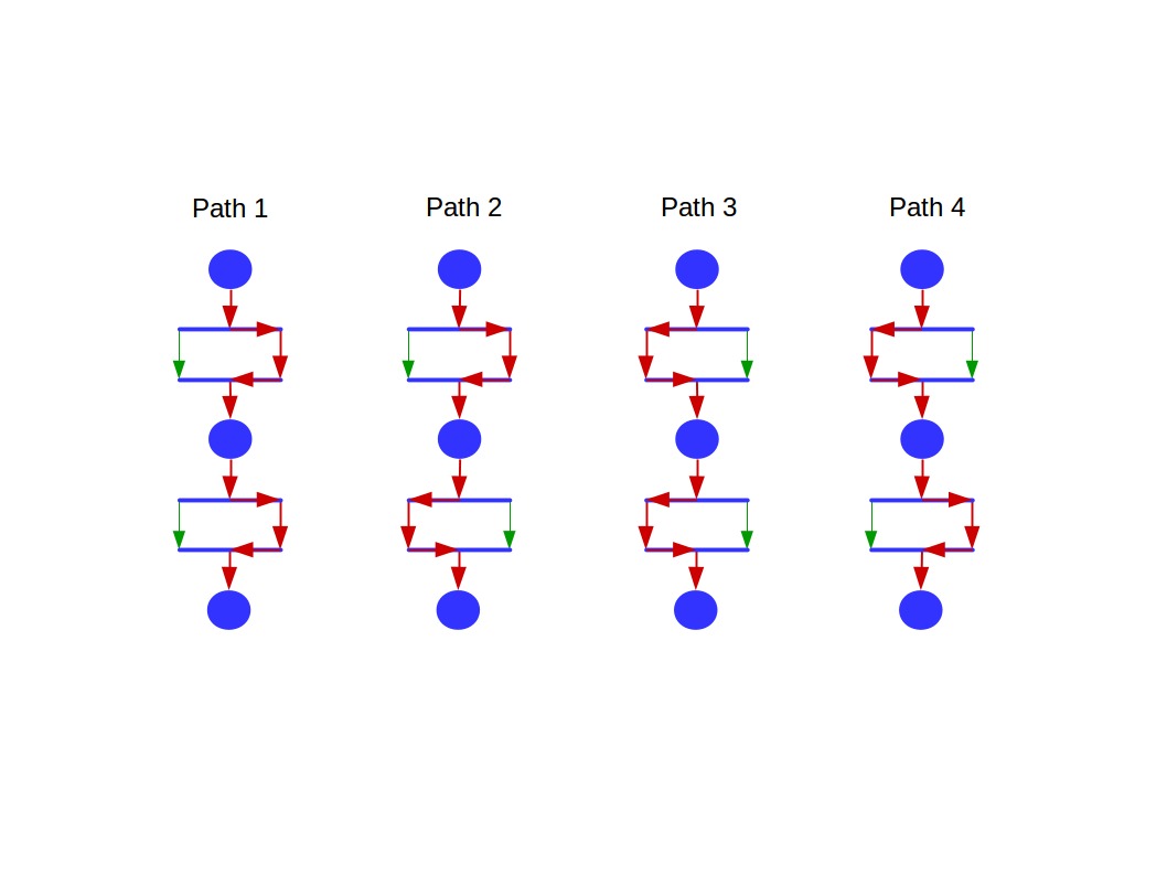
A network using a link with at least two sub links has the following property: for a given input signal only a subset of the network is active. When training is performed, only the weights of the activated sub links are updated. Figure 6 shows a 3-layer network consisting of two links, each link with two sub links. Figure 7 shows this same network with all the possible paths that a signal can take from input to output. It is evident from Figure 7 that there are 4 networks where each network shares some weights with the other networks. It’s easy to over train this type of network since each signal only effects a subset of the weights. To resolve over training the “dropout" regularization technique is used as described in [12].
The key to getting an algorithm working with functions that are discontinuous is a backpropagation algorithm that works for discontinuous functions. The implementation is incredibly simple and the only requirement is to remove idle sub links from the back propagation step. After a signal has been propagated through the network, back propagation is performed, but only on the subset of the network active for the input signal. This means that for each link, only one sub link is active, and so back propagation is performed only on that sub link, all other sub links in the link are ignored. When weights are updated, they are only updated in the links that fired during the forward step.
For clarity we include a description of the back propagation applied to this network, recall that backpropagation is only applied to the active sub network.
- 1.
Forward propagate input signal
- 2.
Record each sub link that is activated for the given input signal
- 3.
Back propagate error signal through active sub links
- 4.
Update weights of the active sub link
- 5.
Ensure that weights are within desired range,
- 6.
Repeat with a new input signal
The error at the output of the network is measured as
The derivative of a link output with respect to a link input is given by
Although, is discontinuous at points, it is entirely continuous within the range of the derivative. If the derivative happens to be required exactly at the discontinuity, the derivative is taken only in the activated sub link (either left or right of the discontinuity). The derivative across a unit to one of the unit input links is
The derivative of the weight with respect to the link output is
Error at the top of the link in the output link
Error at the top of the link one layer in
In the specific case of an averaging unit, the error is
The rule one layer in can be applied to all further layers. The error in the weight is then
At this point, all weight update rules that work for standard neural networks will work for this algorithm as well. A simple example is the momentum update
Although the simple update works for this problem, we instead use Schaul’s parameter free update [30].
2.2 Accelerated Backpropagation
The backpropagation algorithm described is the standard algorithm applied to this model. It was pointed out by [1] that a simple modification to the back propagation algorithm distributes the error more evenly among units. In particular, the algorithm shown suggests that an error at the unit is times the error at the top of the output link (the links leaving the unit). The error at the output of the unit is distributed evenly over the input links, and therefore the more input links there are, the smaller the error that each input link receives. A simple way to remedy this problem is to replace the back propagation (one over the number of active links entering a unit) with (one over the number of links leaving a unit) which will result in a more even distribution of weight change throughout the network and faster convergence. This technique is used in this paper.

2.3 Weight Initialization
2.4 Choosing Ranges and
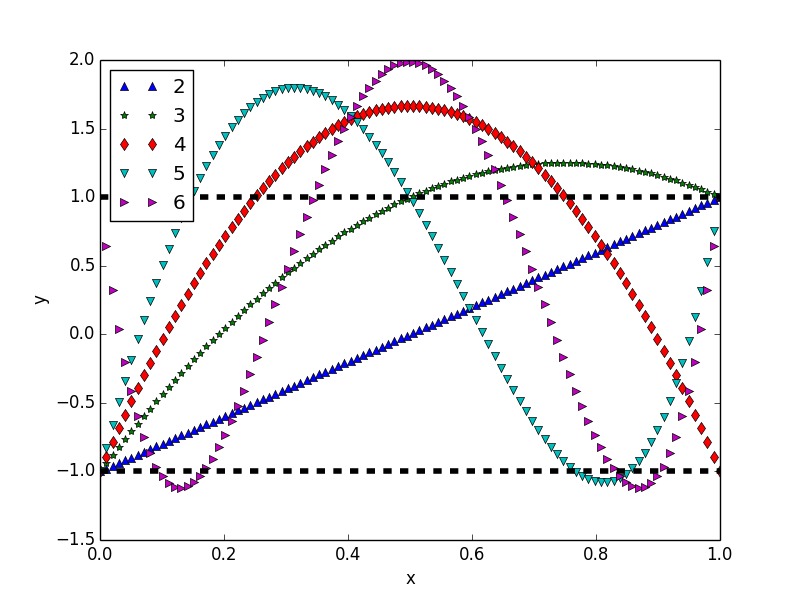
Choosing proper ranges for the links is key to getting good solutions. The weights used in the Lagrange polynomial interpolation do not mark the limits of the polynomial value except in the linear case. Figure 8 shows 5 Lagrange polynomials with maximum overshoot for weights within the desired range - note that only in the linear case is the range limited by the values of the weights. Instead, if the weights are in the range then a given choice of weights will produce a maximum overshoot where values of are given in Table 2. For a given input, the maximum possible output would be which could then be the input to the next link. The input range for each link should be set to to account for these overshoots. One potential consequence of this choice of range is input value decay. Consider a deep network with only one unit per layer and one link between units. Each layer is initialized using Equation (3) with and input range Suppose the input value is then as the input value passes through each layer it will be compressed if by the ratio . After passing through layers, the output signal will be . As a consequence, the output from each layer is pushed towards the value 0 which means fewer and fewer of the network sub links are used. Fortunately, two things can occur to help the situation: (1) if a discontinuity is at the origin rapid learning can still occur since if a signal is either side of 0 it will adjust disconnected weights; (2) as the network is trained, more and more of the sub links are used. It would seem randomly initializing the weights could alleviate this problem, however, we’ve found that symmetric initialization as in Equation (3) works better. In this paper we use where is provided in Table 2 which gives the maximum overshoot for the polynomials when the weights are constrained to be between 1 and -1.
| number of points | 2 | 3 | 4 | 5 | 6 | 7 | 8 | 9 | 10 |
|---|---|---|---|---|---|---|---|---|---|
| 1 | 1.25 | 1.667 | 1.799 | 1.989 | 2.083 | 2.203 | 2.275 | 2.362 |
2.5 Automatic Normalization
Since input links and output links are used in this network and the range and weight is arbitrary, data does not need to be normalized before passing to the network. Normalization automatically occurs for input links by the user’s choice of and for the input links, and by the users choice of and for the output links (see Figure 1 for definitions of input and output links). For example, if the MNIST data is being used and image values range from 0 to 255, simply set and in the input link. Similarly, if the output values should be between 0 and 100 then set the weight limits in the output link to and . Although not particularly important, this is a convenient way to deal with input and output without a separate normalization step.
3 Results
In this section we use the network on 3 problems. The first is the simple sine wave to illustrate how the functional link approximates this function. This provides clarity for how the link in this network differs from the single weight used in the standard approach. The second problem uses the MAGIC gamma ray detection data set to predict if a gamma ray has been detected or not. Finally, results for the MNIST problem are computed with 10 autoencoder classifiers (one for each digit) in a manner similar to that described in [15], though using the reconstruction error to determine the digit. All results are computed using online backpropagation. In this problem, all input and output links have fixed weights and the link function is linear with and . Input links have a range dependent on the range of the input parameters. 50% dropout is used in all cases except the sin wave which only uses one link.
3.1 Sine Wave
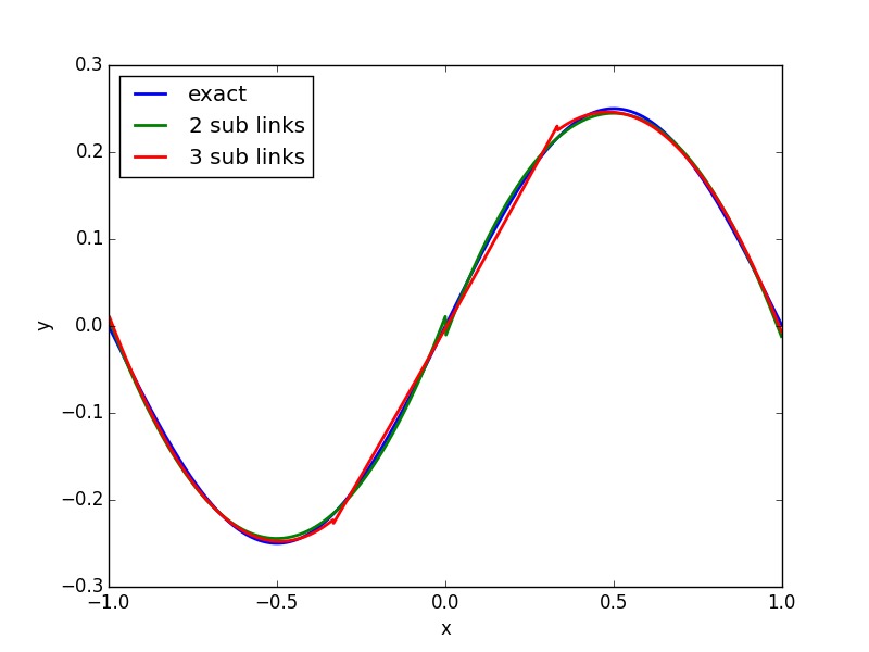
A sine wave is approximated using a single link with several sub links showing the function approximation capability of a single link. This problem is illustrative of how the functions in each sub link are combined to produce the full function. Figure 9 shows a sine wave approximated using a bundle with 3 and 5 linear sub links where discontinuity is allowed between the sub links. Figure 10 shows the same sine wave approximated using a link with 2 and 3 quadratic sub links with discontinuity between them. Note that the linear approximation has 6, and 10 degrees of freedom (for 3 and 5 ranges) and the quadratic approximation has 6 and 9 degrees of freedom (for 2 and 3 ranges). Despite having fewer degrees of freedom the quadratic approximation is substantially better than the linear approximation. This just illustrates the fact that higher order polynomial approximations require fewer degrees for freedom (for the same accuracy) than lower order approximations during function approximation.

3.2 Gamma Ray Detection
The gamma ray detection data is data created to simulate the detection of gamma rays in a ground based atmospheric Cerenkov gamma ray telescope. There are 19,020 examples, where 2/3 of the data is used for training and validation and the remaining 1/3rd is used for testing. The data is shuffled 10 times using a different set for training and test. In the validation runs the 10% of the training data is used as the validation set.
The data can be obtained from the University of California Irvine repository [21]. In the results that follow a parameters scan for network geometry [3, 5, 10, 20, 80, 160] neurons in the layer and with [1, 2, 3, 4, 5, 6, 7, 8] layers, number of sub links was varied from 1 to 6 over one epoch and with to . The solution that produced the best validation accuracy was the case with 80 units in the hidden layers, and 2 sub links. Using this network geometry we then ran to for 50 epochs, using 10 separate test and training sets. The results are shown in Table 3. Table 5 shows previously published results using a decision tree with softening splits[3] for comparison. Table 4 gives the confidence scores as a percent chance that the means of the in the columns and the means of the in the rows actually match for the results of table 3.
Table 3 shows that piecewise linear does not perform nearly as well as the higher solutions. The performance on this problem reaches a minimum around . In particular, the performance improvement from to is about 25%. A key difference between the piecewise linear case and the higher order interpolations is that even after N layers are added to the network, the output of a piecewise linear network, is still piecewise linear, where as if an nth order polynomial is used (for ) as the link function, the output polynomial function is of order where is the number of layers of links.
| test error | ||
|---|---|---|
| 2 | 0.2065 | 0.0225 |
| 3 | 0.1474 | 0.0076 |
| 4 | 0.1368 | 0.0053 |
| 5 | 0.1311 | 0.0039 |
| 6 | 0.1318 | 0.0041 |
| 2 | 3 | 4 | 5 | |
|---|---|---|---|---|
| 3 | 1.0e-3 | |||
| 4 | 3.1e-4 | 3.8e-1 | ||
| 5 | 2.9e-4 | 6.2e-3 | 2.4 | |
| 6 | 3.2e-4 | 1.0e-2 | 4.9 | 100 |
| test error | |
| 0.1376 | 0.00087 |
3.3 Handwritten Digit Recognition
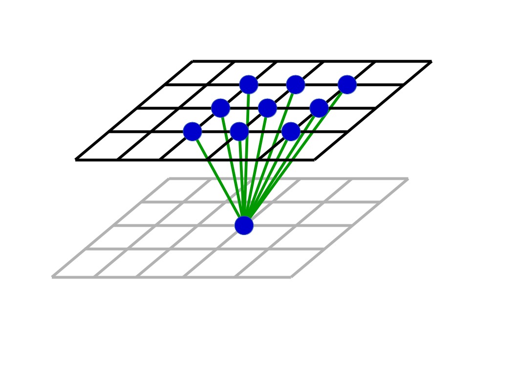
The MNIST is a standard benchmark of neural network codes on optical character recognition [19]. The MNIST data set consists of a 60,000 image training set of 10 digits written from NIST employees and high schoolers. In addition there is a 10,000 image test set that is used to test the generalization capability of the network after the network is trained on the training set. During parameter scans the test set is randomly split into test and validation groups with 50000 in the test groups and 10000 examples in the validation groups. The images consist of 28X28 pixel 1 byte/pixel gray scale images. As such, there are 728 input links (one for each input pixel) and 728 output links. 3 hidden layer are used in the result that are presented with a width of 7 as defined in 11. The digit recognition problem is solved using an autoencoder for each digit. There are 10 autoencoders trained with each of the 10 digits. The Autoencoder 0 is only trained on the digit 0 examples, autoencoder 1 is only trained on the digit 1 examples etc… At the end, the test set examples are run through each autoencoder, the predicted digit is determined by the autoencoder that produces the smallest error for the given input. The error used in this paper is reconstruction error, improvements in this error measure for this approach to classification are explored in [15].
Parameter scans were performed by varying the number of sub links from 1 to 14. The width was varied from 2 to 7 and was varied from 2 to 6. The best configuration validation results are presented in Table 6 with results based on the results of 10 different validation and test sets based on shuffling of the 60,000 example complete test set.
- 1.
- the number of Chebyshev-Lobatto points in the interpolation.
- 2.
layers - the number of neurons in each hidden layer.
- 3.
sub links - the number of sub links in each link.
- 4.
width - the width of the stencil as defined in Figure 11.
| sub links | validation error | ||
|---|---|---|---|
| 2 | 12 | 0.07124 | 0.00276 |
| 3 | 10 | 0.05063 | 0.00293 |
| 4 | 10 | 0.04804 | 0.00216 |
| 5 | 6 | 0.04762 | 0.00271 |
| 6 | 6 | 0.04879 | 0.00295 |
| 2 | 3 | 4 | 5 | |
|---|---|---|---|---|
| 3 | 1.5e-9 | |||
| 4 | 2.3e-11 | 6.1 | ||
| 5 | 8.6e-11 | 4.7 | 100 | |
| 6 | 4.0e-10 | 29 | 83 | 60 |
Table 6 shows MNIST results for varying the number of neighbors used in the multi-layer autoencoder. At a width of 7, a signal from the upper left corner of the input image is able to interact with the signal from the lower right. T-test were performed to measure the significance of the difference in the measured means, see Table 7. In this particular problem it was shown that all cases with were much better than the case with . In addition and was significantly better than assuming a risk of 7%. However, the difference in and is statistically insignificant. Also, note that is not significantly better than .
Recall, that for larger not only does the order of accuracy increase, but also the amount of compression (see Table 2). This means that although the order of accuracy is increasing the network inputs may be being compressed to a smaller region of the polynomial, and therefore reducing the effectiveness of increasing the order of accuracy. In Table 6 the number of sub links is always an even number, this is because an odd number of sub links typically gives a worse solution than an even number. It’s thought that there are 2 causes for this. (1) In deep networks the initial weight values are random values about 0 and the output of each link is averaged at the unit which tends to focus that output around the value 0. As the number of layers is increased the output of each unit approaches 0 more closely. If an odd number of sub links are used, the link function is smooth at 0. If an even number of sub links are used then there is a discontinuity at 0. The discontinuity near the origin means that the solution can rapidly jump between different sub networks and prevents the much slower convergence that is observed with an odd number of sub links. As such, it’s important that a discontinuity should occur at the origin.
| sub links | training error | test error | |
|---|---|---|---|
| 5 | 6 | 0.007183 | 0.0145 |
Table 8 shows the best case from the validation tests in Table 6 run out to 50 epochs. Here we achieve a test error rate of 1.45%, which can be compared with [15] and [14] which show results of 1.27% and 1.1% respectively. Despite the performance discrepancy on this problem we do believe that there are a huge number of options for improving performance. This simplest thing to do would be to add in the non-linearity at the neuron. In this case, to keep the polynomial nature of the network, we suggest using the rectified linear unit. In addition, as the network approaches convergence the network for a given input settles on a single sub network. In this case, that network can be described by a smooth polynomial. This suggest that a non-convex optimization technique should be used (even for the case of 0 discontinuities) and one might be able to take advantage of techniques specifically designed for high order polynomials such as [17] or [18]. Techniques for improving the performance are left as future work.
3.4 Timing Results
A critical question is how much computational time is added for . Both the derivatives and function evaluations become more complex as increases. Furthermore, it might seem that adding additional sub links should increase the computational time. Theoretically, adding new sub links does not increase the time for a single iteration. With evenly spaced sub links the active sub link is determined in O(1) time, so it’s independent of the number of sub links. However, adding new sub links does change the memory usage and structure and can increase inefficiencies that way.
In Tables 9 and 10 below we run the MNIST problem as above with 5 layers, and width 6 with the other parameters specified in the table. The results were computed by running the test case 10 times and averaging the main loop time. Adding additional sub links is not cost free, with 6 sub links is 12% slower than with 2 sub links, but with 3 times the degrees of freedom - this is despite the fact the only one sub link is ever active. In addition increasing the number of sub links with to 12 and the time jumps to 111 seconds (122% slower than with 2 sub links) for 1000 iterations. Despite this fact, the user still gets greater computational power without significantly increasing computational time. Table 9 shows that is only 2.2 times slower than despite having 3 times the degrees of freedom. Similarly, in Table 10 with the same number of degrees of freedom is only 1.83 times slower on average.
| sub links | (seconds) | ||
|---|---|---|---|
| 2 | 2 | 50 | 1 |
| 3 | 2 | 61 | 1.2 |
| 4 | 2 | 77 | 1.5 |
| 5 | 2 | 90 | 1.8 |
| 6 | 2 | 108 | 2.2 |
| sub links | (seconds) | ||
|---|---|---|---|
| 2 | 6 | 59 | 1.0 |
| 3 | 4 | 65 | 1.1 |
| 4 | 3 | 90 | 1.5 |
| 6 | 2 | 108 | 1.8 |
4 Conclusion
A novel approach to artificial neural networks is described where the traditional neuronal non-linearity is eliminated in favor of a discontinuous piecewise polynomial discretization of the weights space of each link. The use of discontinuous piecewise polynomial approximations leads to a network, which is the superposition of multiple networks with a set of shared weights as only a subset of the total network is active for each input signal. Standard backpropagation is used for error correction with the modification that sub links that do not fire are not included in the backpropagation step. The dropout technique [12] is used to minimize over fitting. It is found that piecewise quadratic polynomials generally produce much better results than piecewise linear for the same number of degrees of freedom and that moving to increasingly higher order polynomials can provide additional improvement. We have successfully demonstrated good solutions to the MAGIC and MNIST data sets and expect more complicated problems can be solved as well using this algorithm. Future work will include the addition of a neuronal non-linearity as well as investigation of non-convex optimization techniques.
References
- [1] Igor Aizenberg and Claudio Moraga. Multilayer feedforward neural network based on multi-valued neurons (mlmvn) and a backpropagation learning algorithm. Soft Computing, 11(2):169–183, 2007.
- [2] Yoshua Bengio. Learning deep architectures for ai. Foundations and trends® in Machine Learning, 2(1):1–127, 2009.
- [3] Jakub Dvořák and Petr Savickỳ. Softening splits in decision trees using simulated annealing. In Adaptive and Natural Computing Algorithms, pages 721–729. Springer, 2007.
- [4] Mehdi Fallahnezhad, Mohammad Hassan Moradi, and Salman Zaferanlouei. A hybrid higher order neural classifier for handling classification problems. Expert Systems with Applications, 38(1):386–393, 2011.
- [5] Alhussein Fawzi, Omar Fawzi, and Pascal Frossard. Analysis of classifiers’ robustness to adversarial perturbations. arXiv preprint arXiv:1502.02590, 2015.
- [6] Gian Luca Foresti and T Dolso. An adaptive high-order neural tree for pattern recognition. Systems, Man, and Cybernetics, Part B: Cybernetics, IEEE Transactions on, 34(2):988–996, 2004.
- [7] M Forti and P Nistri. Global convergence of neural networks with discontinuous neuron activations. Circuits and Systems I: Fundamental Theory and Applications, IEEE Transactions on, 50(11):1421–1435, 2003.
- [8] Abram L Friesen and Pedro Domingos. Recursive decomposition for nonconvex optimization. In Proceedings of the 24th International Joint Conference on Artificial Intelligence, 2015.
- [9] Ricard Gavalda and Hava Siegelmann. Discontinuities in recurrent neural networks. Neural computation, 11(3):715–745, 1999.
- [10] C Lee Giles and Tom Maxwell. Learning, invariance, and generalization in high-order neural networks. Applied optics, 26(23):4972–4978, 1987.
- [11] Geoffrey E Hinton and Ruslan R Salakhutdinov. Reducing the dimensionality of data with neural networks. Science, 313(5786):504–507, 2006.
- [12] Geoffrey E Hinton, Nitish Srivastava, Alex Krizhevsky, Ilya Sutskever, and Ruslan R Salakhutdinov. Improving neural networks by preventing co-adaptation of feature detectors. arXiv preprint arXiv:1207.0580, 2012.
- [13] Guang-Bin Huang, Qin-Yu Zhu, and Chee-Kheong Siew. Extreme learning machine: a new learning scheme of feedforward neural networks. In Neural Networks, 2004. Proceedings. 2004 IEEE International Joint Conference on, volume 2, pages 985–990. IEEE, 2004.
- [14] Ozan Irsoy and Ethem Alpaydın. Autoencoder trees. arXiv preprint arXiv:1409.7461, 2014.
- [15] Hanna Kamyshanska and Roland Memisevic. On autoencoder scoring. In Proceedings of the 30th International Conference on Machine Learning (ICML-13), pages 720–728, 2013.
- [16] Stephen H Lane, David A Handelman, and Jack J Gelfand. Theory and development of higher-order cmac neural networks. Control Systems, IEEE, 12(2):23–30, 1992.
- [17] Jean B Lasserre. Global optimization with polynomials and the problem of moments. SIAM Journal on Optimization, 11(3):796–817, 2001.
- [18] Monique Laurent. Sums of squares, moment matrices and optimization over polynomials. In Emerging applications of algebraic geometry, pages 157–270. Springer, 2009.
- [19] Yann LeCun, Léon Bottou, Yoshua Bengio, and Patrick Haffner. Gradient-based learning applied to document recognition. Proceedings of the IEEE, 86(11):2278–2324, 1998.
- [20] Moshe Leshno, Vladimir Ya Lin, Allan Pinkus, and Shimon Schocken. Multilayer feedforward networks with a nonpolynomial activation function can approximate any function. Neural networks, 6(6):861–867, 1993.
- [21] M. Lichman. UCI machine learning repository, 2013.
- [22] Xiaoyang Liu and Jinde Cao. Robust state estimation for neural networks with discontinuous activations. Systems, Man, and Cybernetics, Part B: Cybernetics, IEEE Transactions on, 40(6):1425–1437, 2010.
- [23] Volodymyr Mnih, Koray Kavukcuoglu, David Silver, Andrei A Rusu, Joel Veness, Marc G Bellemare, Alex Graves, Martin Riedmiller, Andreas K Fidjeland, Georg Ostrovski, et al. Human-level control through deep reinforcement learning. Nature, 518(7540):529–533, 2015.
- [24] Vinod Nair and Geoffrey E Hinton. Rectified linear units improve restricted boltzmann machines. In Proceedings of the 27th International Conference on Machine Learning (ICML-10), pages 807–814, 2010.
- [25] Yoh-Han Pao. Adaptive pattern recognition and neural networks. Addison-Wesley Longman Publishing Co., Inc., 1989.
- [26] Jagdish C Patra and Alex C Kot. Nonlinear dynamic system identification using chebyshev functional link artificial neural networks. Systems, Man, and Cybernetics, Part B: Cybernetics, IEEE Transactions on, 32(4):505–511, 2002.
- [27] Jagdish Chandra Patra, Ranendal N Pal, BN Chatterji, and Ganapati Panda. Identification of nonlinear dynamic systems using functional link artificial neural networks. Systems, Man, and Cybernetics, Part B: Cybernetics, IEEE Transactions on, 29(2):254–262, 1999.
- [28] Shubhi Purwar, Indra Narayan Kar, and Amar Nath Jha. On-line system identification of complex systems using chebyshev neural networks. Applied Soft Computing, 7(1):364–372, 2007.
- [29] David E Rumelhart, Geoffrey E Hinton, and Ronald J Williams. Learning representations by back-propagating errors. Cognitive modeling, 1988.
- [30] Tom Schaul, Sixin Zhang, and Yann LeCun. No more pesky learning rates. In Proceedings of The 30th International Conference on Machine Learning, pages 343–351, 2013.
- [31] Yoan Shin and Joydeep Ghosh. Approximation of multivariate functions using ridge polynomial networks. In Neural Networks, 1992. IJCNN., International Joint Conference on, volume 2, pages 380–385. IEEE, 1992.
- [32] Nitish Srivastava, Geoffrey Hinton, Alex Krizhevsky, Ilya Sutskever, and Ruslan Salakhutdinov. Dropout: A simple way to prevent neural networks from overfitting. The Journal of Machine Learning Research, 15(1):1929–1958, 2014.
- [33] Daniel E. Wilson, David E. Whitney, Benjamin Scholl, and David Fitzpatrick. Orientation selectivity and the functional clustering of synaptic inputs in primary visual cortex. Nat Neurosci, advance online publication SP - EP -, Jun 2016. Article.
- [34] Jim YF Yam and Tommy WS Chow. A weight initialization method for improving training speed in feedforward neural network. Neurocomputing, 30(1):219–232, 2000.
- [35] Ming Zhang, Shuxiang Xu, and John Fulcher. Neuron-adaptive higher order neural-network models for automated financial data modeling. Neural Networks, IEEE Transactions on, 13(1):188–204, 2002.