跳到论文正文
W Papers独立论文阅读器 arXiv:1505.03864 论文正文 计算阅读时间 · 0%
引用这篇论文根据当前论文元数据生成,正式投稿前建议核对。


License: arXiv.org perpetual non-exclusive license
arXiv:1505.03864v1 [astro-ph.HE] 14 May 2015

On the primary beam deceleration in the pulsar wind

On the primary beam deceleration in the pulsar wind–B2015
L. I. Arzamasskiy ††thanks: E-mail: lev.arzamasskiy@phystech.edu, beskin@lpi.ru Affiliation: Moscow Institute of Physics and Technology, Dolgoprudny, Institutsky per., 9, Moscow region, 141700, Russia    V. S. Beskin11footnotemark: 1 Affiliation: Moscow Institute of Physics and Technology, Dolgoprudny, Institutsky per., 9, Moscow region, 141700, Russia Affiliation: P.N.Lebedev Physical Institute, Leninsky prosp., 53, Moscow, 119991, Russia    V. V. Prokofev Affiliation: Moscow Institute of Physics and Technology, Dolgoprudny, Institutsky per., 9, Moscow region, 141700, Russia
Accepted. Received; in original form
Abstract

We investigate the motion of the primary beam outside the light cylinder in the pulsar wind. Inside the light cylinder both primary and secondary plasma move along dipole magnetic field lines where their energies can be arbitrary. But at larger distances the theory predicts quasi-radial motion with the velocity exactly corresponding to the drift velocity which cannot be the same for primary and secondary plasma. Hence, the deceleration of the primary beam is to take place simultaneously resulting in the acceleration of the secondary plasma. We investigate this process in the three-fluid MHD approximation and demonstrate that for most pulsars the energy of the beam remains practically unchanged. Only for young radio pulsars (Crab, Vela) essential deceleration up to the energy of the secondary plasma takes place outside the fast magnetosonic surface rF∼(10CLOSEr_{\rm F}\sim(10–OPEN100)​RL100)R_{\rm L}, the energy of secondary plasma itself increasing insufficiently.

Keywords: 
Neutron stars – radio pulsars

1 Introduction

According to the common point of view, the activity of radio pulsars is connected with the electron-positron plasma generated near magnetic poles (Manchester & Taylor, 1977; Smith, 1977). Numerous works devoted to this subject (Sturrock, 1971; Ruderman & Sutherland, 1975; Arons, 1981; Daugherty & Harding, 1982; Gurevich & Istomin, 1985; Istomin & Sobyanin, 2007; Medin & Lai, 2007; Timokhin & Arons, 2013) demonstrate that the outflowing plasma consists of the primary beam with the Lorentz-factor γb∼107\gamma^{\rm b}\sim 10^{7} and the number density nb≈nGJn^{\rm b}\approx n_{\rm GJ}, where nGJ=Ω​B/2​π​c​en_{\rm GJ}=\Omega B/2\pi ce is the Goldreich-Julian number density, and the secondary electron-positron plasma with n±∼(103CLOSEn^{\pm}\sim(10^{3}–OPEN105)​nGJ10^{5})n_{\rm GJ}, and γ±∼102\gamma^{\pm}\sim 10^{2}.

It is clear that inside the light cylinder r<RL=c/Ωr<R_{\rm L}=c/\Omega both the primary beam and the secondary plasma move along the dipole magnetic field lines where their energies can be arbitrary. On the other hand, at large enough distances from a neutron star r≫RLr\gg R_{\rm L} both the analytical theory (Michel, 1994; Beskin et al., 1998) and numerical simulations  (Contopoulos et al., 1999; Spitkovsky, 2006; Tchekhovskoy et al., 2013; Philippov & Spitkovsky, 2014) predict the quasi-radial outflow of the relativistic electron-positron plasma along the poloidal magnetic field with the radial velocity exactly corresponding to the drift motion

𝐔dr=c​𝐄×𝐁B2.{\bf U}_{\rm dr}=c\frac{{\bf E}\times{\bf B}}{B^{2}}. (1)

Clearly, this drift velocity cannot describe simultaneously the motion to the beam and the secondary plasma which have sufficiently different energies.

Thus, the question arises about the energy evolution of these two components as they escape the pulsar magnetosphere and propagate outwards forming the pulsar wind. We show that efficient deceleration of primary beam can be realized for young energetic radio pulsars (Crab, Vela) only. In this case the deceleration up to the energy of the secondary plasma takes place outside the fast magnetosonic surface rF∼(10CLOSEr_{\rm F}\sim(10–OPEN100)​RL100)R_{\rm L}, the energy of secondary plasma itself increases insufficiently. For ordinary pulsars with period P∼1P\sim 1 s, the energy of the primary beam (due to escaping to the region with rather small electric and magnetic fields) remains practically unchanged.

The paper is organized as follows. We start with the description of basic equations of three-fluid MHD in Sect. 2. In Sect. 3 we describe the general properties of these equations. The beam damping is discussed in Sect. 4. Finally, in Sect. 5 the main results of our consideration are formulated.

2 Basic Equations

In this section we derive the basic three-fluid MHD equations. Throughout the paper we use the spherical coordinate system (r,θ,φ)(r,\theta,\varphi) with unit vectors (𝐞r,𝐞θ,𝐞φ)({\bf e}_{r},{\bf e}_{\theta},{\bf e}_{\varphi}). All quantities having the superscript ’b\rm b’ correspond to the primary beam, and the quantities with superscript ’±\pm’ refer to the secondary plasma particles (electrons or positrons). Finally, electron charge equals −e-e.

To describe the deceleration of the primary beam (and possible acceleration of the secondary plasma) we start from the well-known Michel (1994) monopole force-free solution

Br\displaystyle B_{r} =BL​RL2r2,\displaystyle=B_{\rm L}\frac{R_{\rm L}^{2}}{r^{2}}, (2)
Eθ\displaystyle E_{\theta} =Bφ=−BL​RLr​sin⁡θ,\displaystyle=B_{\varphi}=-B_{\rm L}\frac{R_{\rm L}}{r}\sin\theta, (3)

corresponding to the zero particle mass mem_{\rm e}. Within this approximation, the particles move radially with the velocity v=cv=c, so that the current density jr=c​ρej_{r}=c\rho_{\rm e} and the charge density

ρe=−Ω​Br2​π​c​cos⁡θ\rho_{\rm e}=-\frac{\Omega B_{r}}{2\pi c}\cos\theta (4)

just corresponding to Goldreich-Julian charge density

ρGJ=−𝛀​𝐁2​π​c.\rho_{\rm GJ}=-\frac{\bf\Omega B}{2\pi c}. (5)

One can easily check that the fields (2)–(3) with the charge density ρe\rho_{\rm e} (4) and the current density jr=c​ρej_{r}=c\rho_{\rm e} are the exact solutions of the time-independent Maxwell equations

∇⋅𝐄\displaystyle\nabla\cdot{\bf E} =4​π​ρe,∇×𝐄=0,\displaystyle=4\pi\rho_{\rm e},\hskip 8.0pt\nabla\times{\bf E}=0, (6)
∇⋅𝐁\displaystyle\nabla\cdot{\bf B} =0,∇×𝐁=4​πc​𝐣.\displaystyle=0,\hskip 22.0pt\nabla\times{\bf B}=\frac{4\pi}{c}{\bf j}. (7)

For this reason one can model the outflow with the massless particles moving radially with the velocity 𝐯=c​𝐞r{\bf v}=c\,{\bf e}_{r} and having the following number density

n±\displaystyle n^{\pm} =λ​Ω​BL2​π​c​e​RL2r2,\displaystyle=\lambda\frac{\Omega B_{\rm L}}{2\pi ce}\frac{R_{\rm L}^{2}}{r^{2}}, (8)
nb\displaystyle n^{\rm b} =Ω​BL2​π​c​e​RL2r2​cos⁡θ.\displaystyle=\frac{\Omega B_{\rm L}}{2\pi ce}\frac{R_{\rm L}^{2}}{r^{2}}\cos\theta. (9)

Here λ=e​ne/|ρGJ|≫1\lambda=en_{\rm e}/|\rho_{\rm GJ}|\gg 1 is the so-called multiplication parameter which equals 10310^{3}–10510^{5} for most radio pulsars. In what follows we consider for simplicity the case of λ=\lambda= const. Such a choice corresponds to the equality of the secondary electron and positron number densities.

As one can see, the only difference with our previous works (Beskin & Rafikov, 2000; Beskin et al., 2004) is that we consider here not two-component (i.e., secondary electron-positron plasma) but three-component outflow containing also the primary beam having Goldreich-Julian number density nb=|ρGJ|/en^{\rm b}=|\rho_{\rm GJ}|/e and Lorentz-factor γb∼107≫γ±\gamma^{\rm b}\sim 10^{7}\gg\gamma^{\pm}. As is shown in Appendix A, this value is in agreement with the radiation reaction force acting on the beam particle as it moves along dipole magnetic field line inside the light cylinder. On the other hand, as is shown in Appendix B, two-stream instability is not effective, and, hence, three-fluid hydrodynamical approximation under consideration is good enough to describe the evolution of the primary beam.

Then, following the papers mentioned above we can include into consideration the finite particle mass as a small disturbance of the force-free solution. One can do it because for magnetically dominated outflow σ≫1\sigma\gg 1, the outflow remains actually radial (Tomimatsu, 1994; Beskin et al., 1998). Here

σ=Ω​e​BL​RL24​λ​m​c3\sigma=\frac{\Omega eB_{\rm L}R_{\rm L}^{2}}{4\lambda mc^{3}} (10)

is the Michel magnetization parameter. For ordinary pulsars (P∼1P\sim 1 s, B0∼1012B_{0}\sim 10^{12} G), one has σ∼103−104\sigma\sim 10^{3}-10^{4}, and only for the fast ones (P∼0.1−0.01P\sim 0.1-0.01 s, B0∼1013B_{0}\sim 10^{13} G), σ∼105−106\sigma\sim 10^{5}-10^{6}.

As a result, to find the structure of the flow we have to analyze Maxwell equations (6)–(7) and the equation of motion for all three components:

(𝐯±,∇)​𝐩±\displaystyle({\bf v}^{\pm},\nabla){\bf p}^{\pm} =±e⁡(𝐄+𝐯±c×𝐁),\displaystyle=\pm e\left({\bf E}+\frac{{\bf v}^{\pm}}{c}\times{\bf B}\right), (11)
(𝐯b,∇)​𝐩b\displaystyle({\bf v}^{\rm b},\nabla){\bf p}^{\rm b} =−e⁡(𝐄+𝐯bc×𝐁).\displaystyle=-e\left({\bf E}+\frac{{\bf v}^{\rm b}}{c}\times{\bf B}\right). (12)

It is convenient to introduce electric potential Φe​(r,θ)\Phi_{\rm e}(r,\theta) and the magnetic flux function Ψ⁡(r,θ)\Psi(r,\theta), so that

𝐄\displaystyle{\bf E} =−∇Φe​(r,θ),\displaystyle=-\nabla\Phi_{\rm e}(r,\theta), (13)
𝐁p\displaystyle{\bf B}_{\rm p} =∇Ψ×𝐞φ2​π​r​sin⁡θ.\displaystyle=\frac{\nabla\Psi\times{\bf e}_{\varphi}}{2\pi r\sin\theta}. (14)

Then, one can seek the solution in the form

n±\displaystyle n^{\pm} =\displaystyle= Ω​BL2​π​c​e​RL2r2​[λ+η±​(r,θ)],\displaystyle\frac{\Omega B_{\rm L}}{2\pi ce}\frac{R_{\rm L}^{2}}{r^{2}}\left[\lambda+\eta^{\pm}(r,\theta)\right], (15)
nb\displaystyle n^{\rm b} =\displaystyle= Ω​BL2​π​c​e​RL2r2​[cos⁡θ+ηb​(r,θ)],\displaystyle\frac{\Omega B_{\rm L}}{2\pi ce}\frac{R_{\rm L}^{2}}{r^{2}}\left[\cos\theta+\eta^{\rm b}(r,\theta)\right], (16)
Φe​(r,θ)\displaystyle\Phi_{\rm e}(r,\theta) =\displaystyle= Ω​RL2​BLc​[−cos⁡θ+δ⁡(r,θ)],\displaystyle\frac{\Omega R_{\rm L}^{2}B_{\rm L}}{c}\left[-\cos\theta+\delta(r,\theta)\right], (17)
Ψ⁡(r,θ)\displaystyle\Psi(r,\theta) =\displaystyle= 2​π​BL​RL2​[1−cos⁡θ+ε​f​(r,θ)],\displaystyle 2\pi B_{\rm L}R_{\rm L}^{2}\left[1-\cos\theta+\varepsilon f(r,\theta)\right], (18)
vr±,b\displaystyle v^{\pm,{\rm b}}_{r} =\displaystyle= c⁡[1−ξr±,b​(r,θ)],\displaystyle c\left[1-\xi^{\pm,{\rm b}}_{r}(r,\theta)\right], (19)
vθ,φ±,b\displaystyle v^{\pm,{\rm b}}_{\theta,\varphi} =\displaystyle= c​ξθ,φ±,b​(r,θ),\displaystyle c\xi^{\pm,{\rm b}}_{\theta,\varphi}(r,\theta), (20)

with the small disturbances η\eta, δ\delta, ε​f\varepsilon f and ξ\xi corresponding to the small perturbations caused by the finite particle mass. Accordingly, using (13) and (14), one can write down

Br\displaystyle B_{r} =\displaystyle= BL​RL2r2​(1+εsin⁡θ​∂f∂θ),\displaystyle B_{\rm L}\frac{R_{\rm L}^{2}}{r^{2}}\left(1+\frac{\varepsilon}{\sin\theta}\frac{\partial f}{\partial\theta}\right), (21)
Bθ\displaystyle B_{\theta} =\displaystyle= −ε​BL​RL2r​sin⁡θ​∂f∂r,\displaystyle-\varepsilon B_{\rm L}\frac{R_{\rm L}^{2}}{r\sin\theta}\frac{\partial f}{\partial r}, (22)
Bφ\displaystyle B_{\varphi} =\displaystyle= BL​Ω​RLc​RLr​[−sin⁡θ−ζ⁡(r,θ)],\displaystyle B_{\rm L}\frac{\Omega R_{\rm L}}{c}\frac{R_{\rm L}}{r}\left[-\sin\theta-\zeta(r,\theta)\right], (23)
Er\displaystyle E_{r} =\displaystyle= −BL​Ω​RL2c​∂δ∂r,\displaystyle-B_{\rm L}\frac{\Omega R_{\rm L}^{2}}{c}\frac{\partial\delta}{\partial r}, (24)
Eθ\displaystyle E_{\theta} =\displaystyle= BL​Ω​RL2c​r​(−sin⁡θ−∂δ∂θ).\displaystyle B_{\rm L}\frac{\Omega R_{\rm L}^{2}}{cr}\left(-\sin\theta-\frac{\partial\delta}{\partial\theta}\right). (25)

Here all deflecting functions are supposed to be ≪1\ll 1. For vr=cv_{r}=c, vθ=0v_{\theta}=0, and vφ=0v_{\varphi}=0 for all types of particle, we return to the force-free Michel solution.

Now, substituting Eqns. (15)–(25) into Maxwell equtions (6)–(7), we obtain to the first-order approximation the following system of linear equations:

2​(Δ​η+ηb)+∂∂r​(r2​∂δ∂r)+1sin⁡θ​∂∂θ​(sin⁡θ​∂δ∂θ)=0,\displaystyle 2(\Delta\eta+\eta^{\rm b})+\frac{\partial}{\partial r}\left(r^{2}\frac{\partial\delta}{\partial r}\right)+\frac{1}{\sin\theta}\frac{\partial}{\partial\theta}\left(\sin\theta\frac{\partial\delta}{\partial\theta}\right)=0, (26)
12​sin⁡θ​∂∂θ​(ζ​sin⁡θ)=λ​Δ​ξr−ξrb​cos⁡θ−Δ​η−ηb,\displaystyle\frac{1}{2\sin\theta}\frac{\partial}{\partial\theta}(\zeta\sin\theta)=\lambda\Delta\xi_{r}-\xi^{\rm b}_{r}\cos\theta-\Delta\eta-\eta^{\rm b}, (27)
∂ζ∂r=2r​(λ​Δ​ξθ−ξθb​cos⁡θ),\displaystyle\frac{\partial\zeta}{\partial r}=\frac{2}{r}\left(\lambda\Delta\xi_{\theta}-\xi_{\theta}^{\rm b}\cos\theta\right), (28)
εsin⁡θ​∂2f∂r2+εr2​∂∂θ​(1sin⁡θ​∂f∂θ)==2​Ωr​c​(cos⁡θ​ξφb−λ​Δ​ξφ).\displaystyle\begin{split}&\frac{\varepsilon}{\sin\theta}\frac{\partial^{2}f}{\partial r^{2}}+\frac{\varepsilon}{r^{2}}\frac{\partial}{\partial\theta}\left(\frac{1}{\sin\theta}\frac{\partial f}{\partial\theta}\right)=\\ &~~~~~~~~~~~~~~~~~~~~~~~~~~~~~~~=2\frac{\Omega}{rc}\left(\cos\theta\xi^{\rm b}_{\varphi}-\lambda\Delta\xi_{\varphi}\right).\end{split} (29)

Accordingly. equations of motion (11) and (12) now looks like

∂∂r​(ξθ±​γ±)+ξθ±​γ±r==±4​λ​σ​(−1r​∂δ∂θ+ζr−sin⁡θr​ξr±+cΩ​r2​ξφ±),\displaystyle\begin{split}&\frac{\partial}{\partial r}\left(\xi_{\theta}^{\pm}\gamma^{\pm}\right)+\frac{\xi_{\theta}^{\pm}\gamma^{\pm}}{r}=\\ &=\pm 4\lambda\sigma\left(-\frac{1}{r}\frac{\partial\delta}{\partial\theta}\right.\left.+\frac{\zeta}{r}-\frac{\sin\theta}{r}\xi_{r}^{\pm}+\frac{c}{\Omega r^{2}}\xi_{\varphi}^{\pm}\right),\end{split} (30)
∂∂r​(ξθb​γb)+ξθb​γbr==−4​λ​σ​(−1r​∂δ∂θ+ζr−sin⁡θr​ξrb+cΩ​r2​ξφb),\displaystyle\begin{split}&\frac{\partial}{\partial r}\left(\xi_{\theta}^{\rm b}\gamma^{\rm b}\right)+\frac{\xi_{\theta}^{\rm b}\gamma^{\rm b}}{r}=\\ &~~~~~~~=-4\lambda\sigma\left(-\frac{1}{r}\frac{\partial\delta}{\partial\theta}\right.\left.+\frac{\zeta}{r}-\frac{\sin\theta}{r}\xi_{r}^{\rm b}+\frac{c}{\Omega r^{2}}\xi_{\varphi}^{\rm b}\right),\end{split} (31)
∂∂r​(γ±)=±4​λ​σ​(−∂δ∂r−sin⁡θr​ξθ±),\displaystyle\frac{\partial}{\partial r}\left(\gamma^{\pm}\right)=\pm 4\lambda\sigma\left(-\frac{\partial\delta}{\partial r}-\frac{\sin\theta}{r}\xi_{\theta}^{\pm}\right), (32)
∂∂r​(γb)=−4​λ​σ​(−∂δ∂r−sin⁡θr​ξθb),\displaystyle\frac{\partial}{\partial r}\left(\gamma^{\rm b}\right)=-4\lambda\sigma\left(-\frac{\partial\delta}{\partial r}-\frac{\sin\theta}{r}\xi_{\theta}^{\rm b}\right), (33)
∂∂r​(ξφ±​γ±)+ξφ±​γ±r==∓4​λ​σ​(ε​cΩ​r​sin⁡θ​∂f∂r+cΩ​r2​ξθ±),\displaystyle\begin{split}&\frac{\partial}{\partial r}\left(\xi_{\varphi}^{\pm}\gamma^{\pm}\right)+\frac{\xi_{\varphi}^{\pm}\gamma^{\pm}}{r}=\\ &~~~~~~~~~~~~~~~~~~~~=\mp 4\lambda\sigma\left(\varepsilon\frac{c}{\Omega r\sin\theta}\frac{\partial f}{\partial r}\right.\left.+\frac{c}{\Omega r^{2}}\xi_{\theta}^{\pm}\right),\end{split} (34)
∂∂r​(ξφb​γb)+ξφb​γbr==4​λ​σ​(ε​cΩ​r​sin⁡θ​∂f∂r+cΩ​r2​ξθb).\displaystyle\begin{split}&\frac{\partial}{\partial r}\left(\xi_{\varphi}^{\rm b}\gamma^{\rm b}\right)+\frac{\xi_{\varphi}^{\rm b}\gamma^{\rm b}}{r}=\\ &~~~~~~~~~~~~~~~~~~~~=4\lambda\sigma\left(\varepsilon\frac{c}{\Omega r\sin\theta}\frac{\partial f}{\partial r}+\frac{c}{\Omega r^{2}}\xi_{\theta}^{\rm b}\right).\end{split} (35)

Here Δ​A=A+−A−\Delta A=A^{+}-A^{-}, so these terms vanish in one fluid MHD description.

Formally, the system of equations (26)–(35) requires fifteen boundary conditions. We consider for simplicity the case Ω​R/c≪1\Omega R/c\ll 1 when the star radius RR is much smaller than the light cylinder. As a result, one can write down the first nine boundary conditions as

ξθ±​(RL,θ)\displaystyle\xi_{\theta}^{\pm}(R_{\rm L},\theta) =\displaystyle= 0,\displaystyle 0, (36)
ξθb​(RL,θ)\displaystyle\xi_{\theta}^{\rm b}(R_{\rm L},\theta) =\displaystyle= 0,\displaystyle 0, (37)
ξφb​(RL,θ)\displaystyle\xi_{\varphi}^{\rm b}(R_{\rm L},\theta) =\displaystyle= 0,\displaystyle 0, (38)
ξφ±​(RL,θ)\displaystyle\xi_{\varphi}^{\pm}(R_{\rm L},\theta) =\displaystyle= 0,\displaystyle 0, (39)
γ±​(RL,θ)\displaystyle\gamma^{\pm}(R_{\rm L},\theta) =\displaystyle= γin,\displaystyle\gamma_{\rm in}, (40)
γb​(RL,θ)\displaystyle\gamma^{\rm b}(R_{\rm L},\theta) =\displaystyle= γinb,\displaystyle\gamma_{\rm in}^{\rm b}, (41)

where γin\gamma_{\rm in} and γinb\gamma_{\rm in}^{\rm b} are the initial Lorentz-factors of secondary plasma and beam particles correspondingly.

Finally, as a boundary conditions one can put

δ⁡(RL,θ)\displaystyle\delta(R_{\rm L},\theta) =\displaystyle= 0,\displaystyle 0, (42)
ε​f​(RL,θ)\displaystyle\varepsilon f(R_{\rm L},\theta) =\displaystyle= 0,\displaystyle 0, (43)
η+​(RL,θ)−η−​(RL,θ)\displaystyle\eta^{+}(R_{\rm L},\theta)-\eta^{-}(R_{\rm L},\theta) =\displaystyle= 0,\displaystyle 0, (44)
ηb​(RL,θ)\displaystyle\eta^{\rm b}(R_{\rm L},\theta) =\displaystyle= 0,\displaystyle 0, (45)

resulting from the relation 𝐄L+(Ω​RL/c)​𝐞φ×𝐁L=0{\bf E}_{\rm L}+(\Omega R_{\rm L}/c){\bf e}_{\varphi}\times{\bf B}_{\rm L}=0 which implies a rigid rotation and a perfect conductivity of the surface of a star. It is necessary to stress that all the expressions are valid only for a quasi-monopole outflow which exists only outside the light cylinder.

3 General properties

It is clear that in general case the analytical solution of Eqns. (26)–(35) cannot be found. On the other hand, this system of equation contains some integrals of motion which allow us to obtain the necessary information about the energy of the outflowing particles. In particular, as was demonstrate by Beskin & Rafikov (2000), in the two-fluid approximation this approach reproduces well-known one-fluid MHD results for the position of the fast magnetosonic surface for γin≪σ1/3\gamma_{\rm in}\ll\sigma^{1/3}

rF=σ1/3sin−1/3θRLr_{\rm F}=\sigma^{1/3}\sin^{-1/3}\theta\,R_{\rm L} (46)

and the Lorentz-factor at this surface γF=γ±​(rF)\gamma_{\rm F}=\gamma^{\pm}(r_{\rm F})

γF=σ1/3​sin2/3⁡θ.\gamma_{\rm F}=\sigma^{1/3}\sin^{2/3}\theta. (47)

Below we show that it is true for γin≫σ1/3\gamma_{\rm in}\gg\sigma^{1/3} as well.

First of all, excluding ξθ±\xi^{\pm}_{\theta} and ξθb\xi^{\rm b}_{\theta} from Eqn. (28) and using (32) and (33) we obtain the following equation

∂ζ∂r\displaystyle\frac{\partial\zeta}{\partial r} =2tan⁡θ​∂δ∂r−\displaystyle=\frac{2}{\tan\theta}\frac{\partial\delta}{\partial r}-
−12​σ​sin⁡θ​(∂γ+∂r+∂γ−∂r)−12​σ​λ​tan⁡θ​∂γb∂r.\displaystyle-\frac{1}{2\sigma\sin\theta}\left(\frac{\partial\gamma^{+}}{\partial r}+\frac{\partial\gamma^{-}}{\partial r}\right)-\frac{1}{2\sigma\lambda\tan\theta}\frac{\partial\gamma^{\rm b}}{\partial r}. (48)

It gives

ζ−2tan⁡θ​δ+λ⁡(γ++γ−)+(γb−γinb)​cos⁡θ2​λ​σ​sin⁡θ=\displaystyle\zeta-\frac{2}{\tan\theta}\delta+\frac{\lambda(\gamma^{+}+\gamma^{-})+(\gamma^{\rm b}-\gamma_{\rm in}^{\rm b})\cos\theta}{2\lambda\sigma\sin\theta}=
=1σ​sin⁡θ​γin+l⁡(θ)sin⁡θ,\displaystyle=\frac{1}{\sigma\sin\theta}\gamma_{\rm in}+\frac{l(\theta)}{\sin\theta}, (49)

where ζ⁡(0,θ)=l⁡(θ)/sin⁡θ\zeta(0,\theta)=l(\theta)/\sin\theta and l⁡(θ)l(\theta) describes the disturbance of the electric current. Expression (49) corresponds to the conservation of the total energy flux along a magnetic field line. On the other hand, combining Eqns. (32)–(35), one can obtain the expressions corresponding to conversation of the zz-component of the angular momentum for all types of particles

δ\displaystyle\delta =ε​f∓14​λ​σ​γ±​(1−Ω​r​sin⁡θc​ξφ±)±14​λ​σ​γin,\displaystyle=\varepsilon f\mp\frac{1}{4\lambda\sigma}\gamma^{\pm}\left(1-\frac{\Omega r\sin\theta}{c}\xi_{\varphi}^{\pm}\right)\pm\frac{1}{4\lambda\sigma}\gamma_{\rm in}, (50)
δ\displaystyle\delta =ε​f+14​λ​σ​γb​(1−Ω​r​sin⁡θc​ξφb)−14​λ​σ​γinb.\displaystyle=\varepsilon f+\frac{1}{4\lambda\sigma}\gamma^{\rm b}\left(1-\frac{\Omega r\sin\theta}{c}\xi_{\varphi}^{\rm b}\right)-\frac{1}{4\lambda\sigma}\gamma_{\rm in}^{\rm b}. (51)

Now, neglecting the difference between γ+\gamma^{+} and γ−\gamma^{-} so that ξ+=ξ−\xi^{+}=\xi^{-} and γ+=γ−=γ\gamma^{+}=\gamma^{-}=\gamma (which can be done in case of σ≫1\sigma\gg 1 and λ≫1\lambda\gg 1), we obtain

δ=ε​f,\delta=\varepsilon f, (52)

and, hence,

γ⁡(1−Ω​r​sin⁡θc​ξφ)=γin.\gamma\left(1-\frac{\Omega r\sin\theta}{c}\xi_{\varphi}\right)=\gamma_{\rm in}. (53)

Accordingly, from (51) we have

γb​(1−Ω​r​sin⁡θc​ξφb)=γinb.\gamma^{\rm b}\left(1-\frac{\Omega r\sin\theta}{c}\xi^{\rm b}_{\varphi}\right)=\gamma_{\rm in}^{\rm b}. (54)

On the other hand, Eqn. (33) for λ​σ≫1\lambda\sigma\gg 1 gives

−1r​∂δ∂θ+ζr−sin⁡θr​ξr+cΩ​r2​ξφ=0.\displaystyle-\frac{1}{r}\frac{\partial\delta}{\partial\theta}+\frac{\zeta}{r}-\frac{\sin\theta}{r}\xi_{r}+\frac{c}{\Omega r^{2}}\xi_{\varphi}=0. (55)

Further, using the definitions (19)–(20) to describe γ\gamma in terms of ξr\xi_{r} and ξθ\xi_{\theta}, and neglecting ξθ\xi_{\theta}, one can write down

γ2=12​ξr−ξφ2.\gamma^{2}=\frac{1}{2\xi_{r}-\xi_{\varphi}^{2}}. (56)

As a result, combining relations (53), (55), (56), and (56), one can finally find the following algebraic equation on the hydrodynamical Lorentz-factor of the secondary plasma γ\gamma

2​γ3−2​σ​[K+12​x2+γinσ]​γ2+σ​sin2⁡θ+σ​c2​γin2Ω2​r2=0,2\gamma^{3}-2\sigma\left[K+\frac{1}{2x^{2}}+\frac{\gamma_{\rm in}}{\sigma}\right]\gamma^{2}+\sigma\sin^{2}\theta+\sigma\frac{c^{2}\gamma_{\rm in}^{2}}{\Omega^{2}r^{2}}=0, (57)

where x=r/RLx=r/R_{\rm L} and

K⁡(r,θ)=2​cos⁡θ​δ−sin⁡θ​∂δ∂θ−γb−γinb2​σ​λ​cos⁡θ+l⁡(θ)sin⁡θ.K(r,\theta)=2\cos\theta\delta-\sin\theta\frac{\partial\delta}{\partial\theta}-\frac{\gamma^{\rm b}-\gamma_{\rm in}^{\rm b}}{2\sigma\lambda}\cos\theta+\frac{l(\theta)}{\sin\theta}. (58)

Equations (57)–(58) generalize the appropriate ones obtained by Beskin & Rafikov (2000) for two-component plasma and for γin≪σ1/3\gamma_{\rm in}\ll\sigma^{1/3}. As was already stressed, these equations allow us to find the position of fast magnetosonic surface corresponding to the intersection of two roots of algebraic equation (57). Indeed, determining the derivative r​∂γ/∂rr\partial\gamma/\partial r, one can obtain

r​∂γ∂r=γ​σ​r​∂K/∂r−x−2​[1−(γin/γ)2]3​γ−2​γin−σ⁡(2​K+x−2).r\frac{\partial\gamma}{\partial r}=\gamma\sigma\frac{r\partial K/\partial r-x^{-2}[1-(\gamma_{\rm in}/\gamma)^{2}]}{3\gamma-2\gamma_{\rm in}-\sigma(2K+x^{-2})}. (59)

As the fast magnetosonic surface is the XX-point, both the numerator and denominator are both equal to zero there. As a result, evaluating r​∂K/∂rr\partial K/\partial r as KK, we obtain the following well-known asymptotic solutions (Bogovalov, 2001):

  1. 1.

    Fast rotator (γin<σ1/3\gamma_{\rm in}<\sigma^{1/3}). In this case we may neglect the terms containing γin\gamma_{\rm in}. It gives for δF=δ⁡(rF)\delta_{\rm F}=\delta(r_{\rm F}), etc.

    δF\displaystyle\delta_{\rm F} ≈\displaystyle\approx σ−2/3,\displaystyle\sigma^{-2/3}, (60)
    rF\displaystyle r_{\rm F} ≈\displaystyle\approx σ1/3sin−1/3θRL,\displaystyle\sigma^{1/3}\sin^{-1/3}\theta\,R_{\rm L}, (61)
    γF\displaystyle\gamma_{\rm F} =\displaystyle= σ1/3​sin2/3⁡θ,\displaystyle\sigma^{1/3}\sin^{2/3}\theta, (62)

    the last expression being exact. As we see, for fast rotator the acceleration of the secondary plasma from γ=γin\gamma=\gamma_{\rm in} to γ=σ1/3\gamma=\sigma^{1/3} takes place up to the fast magnetosonic surface.

  2. 2.

    Slow rotator (γin>σ1/3\gamma_{\rm in}>\sigma^{1/3}). In this case we obtain

    δF\displaystyle\delta_{\rm F} ≈\displaystyle\approx γin​σ−1,\displaystyle\gamma_{\rm in}\sigma^{-1}, (63)
    rF\displaystyle r_{\rm F} ≈\displaystyle\approx σ1/2γin−1/2RL,\displaystyle\sigma^{1/2}\gamma_{\rm in}^{-1/2}\,R_{\rm L}, (64)
    γF\displaystyle\gamma_{\rm F} ≈\displaystyle\approx γin.\displaystyle\gamma_{\rm in}. (65)

    For slow rotator there is no particle acceleration within the fast magnetosonic surface which has a spherical shape.

4 Beam Damping and Plasma Acceleration

4.1 Beam damping

In this section we determine how the energy of the primary beam changes as it outflows from the pulsar magnetosphere. As we consider the secondary plasma in the MHD limit where there is no longitudinal electric field, we may neglect the term ∂δ/∂r\partial\delta/\partial r. This leads to the simple determination of ξθb\xi_{\theta}^{\rm b} from Eqn. (33):

ξθb≈r4​λ​σ​∂γb∂r,\xi_{\theta}^{\rm b}\approx\frac{r}{4\lambda\sigma}\frac{\partial\gamma^{\rm b}}{\partial r}, (66)

where we also consider the case sin⁡θ∼cos⁡θ∼1\sin\theta\sim\cos\theta\sim 1. On the other hand, for λ​σ≫1\lambda\sigma\gg 1 one can set the quantity in brackets in Eqn. (30) equal to zero. After that we can rewrite Eqn. (31) in the following way:

∂∂r​(r​ξθb​γb)=4​λ​σ​[ξrb−ξr−rRL​(ξφb−ξφ)].\frac{\partial}{\partial r}(r\xi^{\rm b}_{\theta}\gamma^{\rm b})=4\lambda\sigma\left[\xi_{r}^{\rm b}-\xi_{r}-\frac{r}{R_{\rm L}}(\xi_{\varphi}^{\rm b}-\xi_{\varphi})\right]. (67)

Now, using Eqs. (53)–(54), (56) and the definition

ξrb=12​(γb)2+(ξφb)22,\xi_{r}^{\rm b}=\frac{1}{2(\gamma^{\rm b})^{2}}+\frac{(\xi_{\varphi}^{\rm b})^{2}}{2}, (68)

one can finally obtain the following general equation describing the beam damping:

∂∂x​(x2​∂p∂x)=Λ2​(1(γinb)2​1p+1−1γ2−1x2​pp+1+Δx2).\displaystyle\frac{\partial}{\partial x}\left(x^{2}\frac{\partial p}{\partial x}\right)=\Lambda^{2}\left(\frac{1}{(\gamma^{\rm b}_{\rm in})^{2}}\frac{1}{p+1}-\frac{1}{\gamma^{2}}-\frac{1}{x^{2}}\frac{p}{p+1}+\frac{\Delta}{x^{2}}\right). (69)

Here we use the following notations

p=(γb)2−(γinb)2(γinb)2,Λ=4​λ​σγinb,Δ=γ2−γin2γ2.p=\frac{(\gamma^{\rm b})^{2}-(\gamma^{\rm b}_{\rm in})^{2}}{(\gamma^{\rm b}_{\rm in})^{2}},~\Lambda=\frac{4\lambda\sigma}{\gamma^{\rm b}_{\rm in}},~\Delta=\frac{\gamma^{2}-\gamma_{\rm in}^{2}}{\gamma^{2}}. (70)

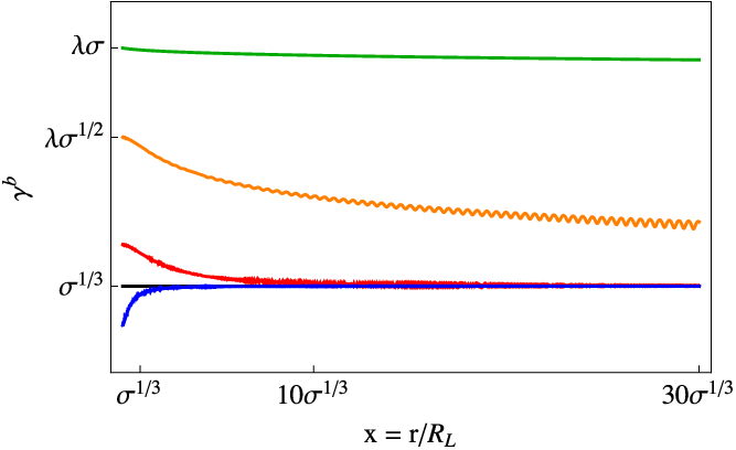
The solutions of equation (69) for different initial energy me​c2​γinbm_{\rm e}c^{2}\gamma_{\rm in}^{\rm b} of a beam (and for γin=γ=σ1/3\gamma_{\rm in}=\gamma=\sigma^{1/3}) are presented on Figure 1. As we see, for very large initial Lorentz-factor of a beam γinb>λ​σ\gamma_{\rm in}^{\rm b}>\lambda\sigma (green line), its energy remains actually constant. The point is that the Larmor radius rL=me​c2​γb/e​BLr_{\rm L}=m_{\rm e}c^{2}\gamma^{\rm b}/eB_{\rm L} for such a large energy of a beam is much larger than the light cylinder radius RLR_{\rm L} so the electromagnetic fields cannot disturb the radial motion of the beam. But, as we see, for γinb≈λ​σ1/2\gamma_{\rm in}^{\rm b}\approx\lambda\sigma^{1/2}, when rL≈RLr_{\rm L}\approx R_{\rm L} (orange line), the curve has oscillations corresponding to rotation in the comoving reference frame and beam energy slightly damps.

On the other hand, for smaller Lorenz-factors of the beam γin<γinb<λ​σ1/2\gamma_{\rm in}<\gamma_{\rm in}^{\rm b}<\lambda\sigma^{1/2} (red line) the beam energy marginally damps to the energy of secondary plasma. Here again the oscillations correspond to the rotation in the comoving reference frame. For γinb=γ=σ1/3\gamma_{\rm in}^{\rm b}=\gamma=\sigma^{1/3} (black line), the energy of the beam remains unchanged. Finally, if the initial energy of the beam is relatively close to the energy of the secondary plasma, the beam either damps or accelerates to the secondary plasma energy. Although the case of γinb<γ\gamma_{\rm in}^{\rm b}<\gamma (blue line) is impossible in real pulsars, this solution describes the behaviour of secondary particles: if their initial Lorentz-factor is less than σM1/3\sigma^{1/3}_{\rm M}, they become accelerated to this energy.
Refer to caption
Figure 1: The evolution of the beam Lorentz-factor γb​(x)\gamma^{\rm b}(x) for different initial energies me​c2​γinbm_{\rm e}c^{2}\gamma_{\rm in}^{\rm b} (see text for more detail).

For sufficiently large initial Lorenz-factors of the beam, one can put p≪1p\ll 1 and neglect the second term in (69). In this case Eqn. (69) becomes linear, and one could solve it using Green’s function:

p⁡(x)=Λ2​∫1xd​x′​sin⁡(Λx−Λx′)​[1γ2​(x′)+Δ⁡(x′)x′2].p(x)=\Lambda^{2}\int\limits_{1}^{x}\text{d}x^{\prime}\sin\left(\dfrac{\Lambda}{x}-\dfrac{\Lambda}{x^{\prime}}\right)\left[\dfrac{1}{\gamma^{2}(x^{\prime})}+\dfrac{\Delta(x^{\prime})}{x^{\prime 2}}\right]. (71)

After transition to the limit x→∞x\rightarrow\infty, we obtain the following asymptotic solution:

p⁡(x)≃−(Λγout)2​[ln⁡(x/Λ)−Γ].p(x)\simeq-\left(\dfrac{\Lambda}{\gamma_{\rm out}}\right)^{2}[\ln(x/\Lambda)-\Gamma]. (72)

Here

γout=limx→∞γ⁡(x),\gamma_{\rm out}=\lim\limits_{x\rightarrow\infty}\gamma(x), (73)

and Γ≃1\Gamma\simeq 1–1010 is a constant which weakly depends on behavior of γ⁡(x)\gamma(x) and Λ\Lambda. For constant γ\gamma and Λ≳1\Lambda\ga 1, this value is equal to the Euler-Mascheroni constant Γ≈0.577\Gamma\approx 0.577.

Approximating now ln⁡(x/Λ)−Γ∼1\ln(x/\Lambda)-\Gamma\sim 1, one can finally obtain the following equation describing Lorentz-factor of the primary particles:

(γoutb)2=(γinb)2−(4​λ​σ/γout)2.(\gamma^{\rm b}_{\rm out})^{2}=(\gamma^{\rm b}_{\rm in})^{2}-(4\lambda\sigma/\gamma_{\rm out})^{2}. (74)

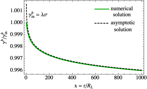
Hence, as was already found, large enough disturbance of the energy of the primary beam Δ​γb≃γinb\Delta\gamma^{\rm b}\simeq\gamma^{\rm b}_{\rm in} is valid only if the condition γinb<λ​σ1/2\gamma^{\rm b}_{\rm in}<\lambda\sigma^{1/2} holds. For γinb>λ​σ\gamma^{\rm b}_{\rm in}>\lambda\sigma the energy of the beam remains actually unchenged. Figure 2 illustrates the evolution of γb​(r)\gamma^{\rm b}(r) according to the numerical solution of Eqn. (69) in comparison with analytical solution (72). As we see, they are in a very good agreement. To summarize, the beam energy stabilizes at the following values:

γoutb\displaystyle\gamma_{\rm out}^{\rm b} =\displaystyle= γout;γinb<λ​σ1/2,\displaystyle\gamma_{\rm out};~~~~~~~~\gamma_{\rm in}^{\rm b}<\lambda\sigma^{1/2}, (75)
γout<γoutb\displaystyle\gamma_{\rm out}<\gamma_{\rm out}^{\rm b} <\displaystyle< γinb;λ​σ1/2<γinb<λ​σ,\displaystyle\gamma_{\rm in}^{\rm b};~~~~~~~~\lambda\sigma^{1/2}<\gamma_{\rm in}^{\rm b}<\lambda\sigma, (76)
γoutb\displaystyle\gamma_{\rm out}^{\rm b} =\displaystyle= γinb;γinb>λ​σ,\displaystyle\gamma_{\rm in}^{\rm b};~~~~~~~~\gamma_{\rm in}^{\rm b}>\lambda\sigma, (77)

where γout\gamma_{\rm out} is the final Lorentz-factor of the secondary plasma (see below).
Refer to caption
Figure 2: Evolution of the Lorenz-factor of the beam for γinb=λ​σ\gamma_{\rm in}^{\rm b}=\lambda\sigma. Green solid line represents numerical solution of exact equation (69) and black dashed line describes analytical asymptotic solution (72).

Note, that if γinb>λ​σ\gamma_{\rm in}^{\rm b}>\lambda\sigma, the pulsar total energy losses are less than the beam energy. This case is thus unphysical.

4.2 Secondary plasma acceleration

We are now in position to evaluate the final Lorentz-factor of the secondary plasma γout\gamma_{\rm out}. For this we look for the solution of equation (57) in the limit x→∞x\rightarrow\infty. Neglecting the disturbance of electric current we can approximate K⁡(r,θ)K(r,\theta) in Eqn. (58) as

K∞=δ∞−γoutb−γinb2​σ​λ.K_{\infty}=\delta_{\infty}-\frac{\gamma^{\rm b}_{\rm out}-\gamma_{\rm in}^{\rm b}}{2\sigma\lambda}. (78)

At large distances outside the fast magnetosonic surface we can neglect two last terms in equation (57), which gives us a simple expression for γout\gamma_{\rm out}:

γout=γin+σ⁡(δ∞−γoutb−γinb2​λ​σ).\gamma_{\rm out}=\gamma_{\rm in}+\sigma\left(\delta_{\infty}-\frac{\gamma^{\rm b}_{\rm out}-\gamma_{\rm in}^{\rm b}}{2\lambda\sigma}\right). (79)

According to Eqns. (60), (63), δ∞∼max(σ−2/3,γinσ−1)\delta_{\infty}\sim\max(\sigma^{-2/3},\gamma_{\rm in}\sigma^{-1}), so we approximate equation (79) as

γout=max⁡(σ1/3,γin)−γoutb−γinb2​λ.\gamma_{\rm out}=\max(\sigma^{1/3},\gamma_{\rm in})-\frac{\gamma^{\rm b}_{\rm out}-\gamma_{\rm in}^{\rm b}}{2\lambda}. (80)

In what follows we consider for simplicitly the case γin≪σ1/3\gamma_{\rm in}\ll\sigma^{1/3}, but our results could be easily generalized for the opposite case.

Note, that equation (80) sets γout\gamma_{\rm out} implicitly since γoutb\gamma_{\rm out}^{\rm b} depends on γout\gamma_{\rm out}:

γoutb−γinb≈(γoutb)2−(γinb)22​γinb=γinb2​pout​(γout).\gamma^{\rm b}_{\rm out}-\gamma_{\rm in}^{\rm b}\approx\frac{(\gamma^{\rm b}_{\rm out})^{2}-(\gamma_{\rm in}^{\rm b})^{2}}{2\gamma_{\rm in}^{\rm b}}=\frac{\gamma_{\rm in}^{\rm b}}{2}p_{\rm out}(\gamma_{\rm out}). (81)

This approximation is valid only when the beam damping is small, i.e., for large enough γinb\gamma_{\rm in}^{\rm b}. In this limit, using equation (72), we finally obtain

γout=σ1/3+4​λ​σ2γinb​γout2.\gamma_{\rm out}=\sigma^{1/3}+\frac{4\lambda\sigma^{2}}{\gamma_{\rm in}^{\rm b}\gamma_{\rm out}^{2}}. (82)

For very large γinb\gamma_{\rm in}^{\rm b}, one can put γout=γin=σ1/3\gamma_{\rm out}=\gamma_{\rm in}=\sigma^{1/3}, so both the beam and the secondary plasma do not change their energy. But there is a range of the value γinb\gamma_{\rm in}^{\rm b}, where the second term in Eqn. (82) is larger than the first one. For such parameters

γout∼λ1/3​σ2/3(γinb)1/3.\gamma_{\rm out}\sim\frac{\lambda^{1/3}\sigma^{2/3}}{(\gamma_{\rm in}^{\rm b})^{1/3}}. (83)

Finally, for sufficiently small γinb\gamma_{\rm in}^{\rm b}, one can put γoutb=σ1/3\gamma_{\rm out}^{\rm b}=\sigma^{1/3}. Then, for λ≫1\lambda\gg 1 equation (80) transforms into

γout=σ1/3+γinb2​λ.\gamma_{\rm out}=\sigma^{1/3}+\frac{\gamma_{\rm in}^{\rm b}}{2\lambda}. (84)

Thus, for small enough initial energy of the beam, the energy of the secondary particles linearly increases with γinb\gamma_{\rm in}^{\rm b} 11 1 For γinb<γin\gamma_{\rm in}^{\rm b}<\gamma_{\rm in}, equation (80) gives γout<γin\gamma_{\rm out}<\gamma_{\rm in}, i.e., the secondary plasma loses energy and accelerates the primary particles.

One can now construct the following approximate expression, which is valid in both limits

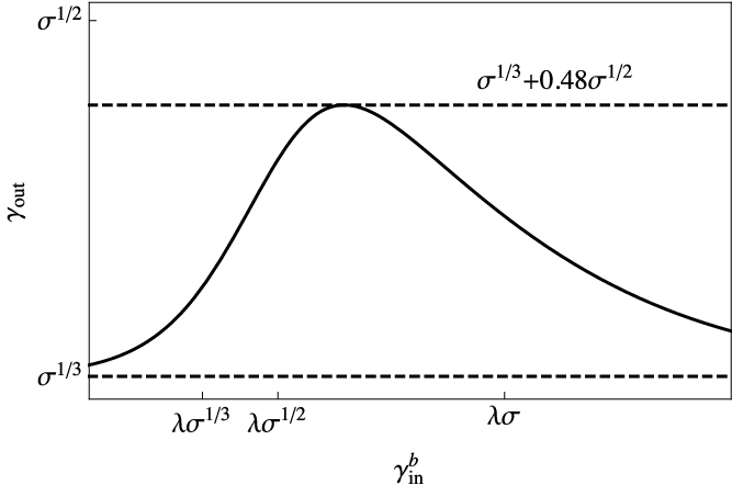
γout=σ1/3+[(γinb2​λ)−1+(λ1/3​σ2/3(γinb)1/3)−1]−1\gamma_{\rm out}=\sigma^{1/3}+\left[\left(\frac{\gamma_{\rm in}^{\rm b}}{2\lambda}\right)^{-1}+\left(\frac{\lambda^{1/3}\sigma^{2/3}}{(\gamma_{\rm in}^{\rm b})^{1/3}}\right)^{-1}\right]^{-1} (85)

and determine the maximum gamma factor of the secondary plasma:

γoutmax∼σ1/2,for​γinb=λ​σM1/2.\gamma_{\rm out}^{\rm max}\sim\sigma^{1/2},~{\rm for}~\gamma_{\rm in}^{\rm b}=\lambda\sigma^{1/2}_{\rm M}. (86)

Figure 3 shows obtained asymptotic behavior (85). The exact location of the maximum is γinb=63/4​λ​σM1/2\gamma_{\rm in}^{\rm b}=6^{3/4}\lambda\sigma^{1/2}_{\rm M} and γoutmax=σM1/3+0.25​(3/8)3/4​σM1/2≈σM1/3+0.48​σM1/2\gamma_{\rm out}^{\rm max}=\sigma^{1/3}_{\rm M}+0.25(3/8)^{3/4}\sigma^{1/2}_{\rm M}\approx\sigma^{1/3}_{\rm M}+0.48\sigma^{1/2}_{\rm M}. One should also note that the maximum gamma-factor of the secondary plasma is close to the initial one: even for the fastest pulsars,

γoutmax/γin=σ1/6∼10.\gamma_{\rm out}^{\rm max}/\gamma_{\rm in}=\sigma^{1/6}\sim 10. (87)

All the expressions written above remains the same in case γin≫σ1/3\gamma_{\rm in}\gg\sigma^{1/3} as well. The only differences is in first terms of r.h.s of Eqns. (82), (84), and (85), which are replaced on γin\gamma_{\rm in} instead of σM1/3\sigma^{1/3}_{\rm M}. This implies that for such pulsars the effect of the pulsar wind acceleration via beam particles is even smaller. For γin≫σM1/2\gamma_{\rm in}\gg\sigma^{1/2}_{\rm M} this effect vanishes.

Refer to caption
Figure 3: The final Lorentz-factor of the secondary plasma according to Eqn. (85).

5 Conclusion

It was demonstrated that the effective deceleration of the primary beam takes place only for relatively small beam energy

γinb<λ​σ1/2.\gamma_{\rm in}^{\rm b}<\lambda\sigma^{1/2}. (88)

As λ\lambda and σ\sigma are connected with the relation (Beskin, 2010)

σ​λ∼(WtotWA)1/2,\sigma\lambda\sim\left(\frac{W_{\rm tot}}{W_{\rm A}}\right)^{1/2}, (89)

where WtotW_{\rm tot} is the total energy losses of a pulsar and WA=me2​c5/e2≈1017W_{\rm A}=m_{\rm e}^{2}c^{5}/e^{2}\approx 10^{17} erg/s, one can easily estimate the total number of pulsars having effective damping of the primary beam. Setting γinb=107\gamma_{\rm in}^{\rm b}=10^{7} and λ=104\lambda=10^{4}, we obtain that among 2003 known radio pulsars with measured PP and P˙\dot{P}, only 65 sources have relatively small initial Lorentz-factors γinb<λ​σ1/2\gamma^{\rm b}_{\rm in}<\lambda\sigma^{1/2}.

Thus, one can conclude that effective deceleration of the primary beam takes place only for sufficiently energetic pulsars satisfying the condition Wtot≳1036W_{\rm tot}\ga 10^{36} erg/s (Crab, Vela). In this case during its motion through the magnetosphere the primary beam decelerates, accelerating simultaneously the secondary particles. But such an additional acceleration is not actually effective enough as the maximum Lorentz-factor of the secondary plasma does not exceed σ1/2\sigma^{1/2}, which is only on the factor σ1/6\sigma^{1/6} larger than the energy of the seconary plasma near the fast magnetosonic surface. For ordinary pulsars the deceleration of the primary beam can be neglected, so the energy of the primary beam as well as secondary plasma remain constant.

It is very important that the deceleration/acceleration takes place on the scale of the fast magnetosonic surface rF∼σ1/3​RLr_{\rm F}\sim\sigma^{1/3}R_{\rm L}, i.e., at the distances much larger than the radius of the light cylinder. This implies that even for the fast young radio pulsars the energetic particles of the beam will intersect the magnetospheric current sheet as their velocities exceed the velocity of the secondary plasma which just determines the radial velocity of the current sheet. Indeed, for fast pulsars the scale rF∼102​RLr_{\rm F}\sim 10^{2}R_{\rm L} corresponds to several wave length of the current sheet.

6 Acknowledgments

We thank A.Spitkovsky, A.Philippov and Y.N. Istomin for their interest and useful discussions. This work was partially supported by Russian Foundation for Basic Research (Grant no. 14-02-00831).

References

  • Arons (1981) Arons J., 1981, ApJ, 248, 1099
  • Beskin (2010) Beskin V. S., 2010, MHD Flows in Compact Astrophysical Objects. Springer
  • Beskin et al. (1998) Beskin V. S., Kuznetsova I. V., Rafikov R. R., 1998, MNRAS, 299, 341
  • Beskin & Rafikov (2000) Beskin V. S., Rafikov R. R., 2000, MNRAS, 313, 433
  • Beskin et al. (2004) Beskin V. S., Zakamska N. L., Sol H., 2004, MNRAS, 347, 587
  • Bogovalov (2001) Bogovalov S. V., 2001, A&A, 371, 1155
  • Contopoulos et al. (1999) Contopoulos I., Kazanas D., Fendt C., 1999, ApJ, 511, 351
  • Daugherty & Harding (1982) Daugherty J. K., Harding A. K., 1982, ApJ, 252, 337
  • Gurevich & Istomin (1985) Gurevich A. V., Istomin I. N., 1985, Zhurnal Eksperimentalnoi i Teoreticheskoi Fiziki, 89, 3
  • Istomin & Sobyanin (2007) Istomin Y. N., Sobyanin D. N., 2007, Astronomy Letters, 33, 660
  • Manchester & Taylor (1977) Manchester R. N., Taylor J. H., 1977, Pulsars. W. H. Freeman
  • Medin & Lai (2007) Medin Z., Lai D., 2007, MNRAS, 382, 1833
  • Michel (1994) Michel F. C., 1994, ApJ, 431, 397
  • Philippov & Spitkovsky (2014) Philippov A. A., Spitkovsky A., 2014, ApJ, 785, L33
  • Ruderman & Sutherland (1975) Ruderman M. A., Sutherland P. G., 1975, ApJ, 196, 51
  • Smith (1977) Smith F. G., 1977, Pulsars. Cambridge University Press
  • Spitkovsky (2006) Spitkovsky A., 2006, ApJ, 648, L51
  • Sturrock (1971) Sturrock P. A., 1971, ApJ, 164, 529
  • Tchekhovskoy et al. (2013) Tchekhovskoy A., Spitkovsky A., Li J. G., 2013, MNRAS, 435, L1
  • Timokhin & Arons (2013) Timokhin A. N., Arons J., 2013, MNRAS, 429, 20
  • Tomimatsu (1994) Tomimatsu A., 1994, PASJ, 46, 123
  • Zheleznyakov (1977) Zheleznyakov V. V., 1977, Electromagnetic waves in cosmic plasma. Generation and propagation. Nauka

Appendix A Radiation force damping

Inside the light cylinder the damping of a beam is defined by radiation losses. Outside the acceleration gap the change of the bulk Lorentz-factor of a beam is described by following equation (Zheleznyakov, 1977)

m​c2​d​γd​l=−23​e2Rc2​γ4,mc^{2}\frac{{\rm d}\gamma}{{\rm d}l}=-\frac{2}{3}\frac{e^{2}}{R_{c}^{2}}\gamma^{4}, (90)

where RcR_{c} is the curvature radius of particle trajectory (i.e., the curvature radius of the magnetic field line), and ll is a path. For simplify we consider here a dipole structure of magnetic field inside the light cylinder.

Dipole magnetic field lines in polar coordinates are described by the well-known relation r=r0​sin2⁡θr=r_{0}\sin^{2}\theta, where r0≳RLr_{0}\ga R_{\rm L} is a parameter of the line. The appropriate expression in Cartesian coordinates looks like y=±(r0​x2)2/3−x2y=\pm\sqrt{(r_{0}x^{2})^{2/3}-x^{2}}. It gives for the curvature radius

Rc=r0​a1/3​(4−3​a2/3)3/2(6−3​a2/3),R_{c}=r_{0}\dfrac{a^{1/3}(4-3a^{2/3})^{3/2}}{(6-3a^{2/3})}, (91)

where a=x/r0a=x/r_{0}. Accordingly,

d​l=r03​4−3​a2/3a2/3​(1−a2/3)​d​a.{\rm d}l=\dfrac{r_{0}}{3}\sqrt{\dfrac{4-3a^{2/3}}{a^{2/3}(1-a^{2/3})}}{\rm d}a. (92)

It gives

d​γγ4=−6​rer0∫R/r0RL/r0d​aa(2−a2/3)2(4−3​a2/3)5/2​(1−a2/3)1/2.\frac{\text{d}\gamma}{\gamma^{4}}=-\frac{6r_{e}}{r_{0}}\int\limits_{R/r_{0}}^{R_{L}/r_{0}}\dfrac{{\rm d}a}{a}\dfrac{(2-a^{2/3})^{2}}{(4-3a^{2/3})^{5/2}(1-a^{2/3})^{1/2}}. (93)

Here re=e2/me​c2r_{\rm e}=e^{2}/m_{\rm e}c^{2} is the classical electron radius, and RR is the stellar radius. This equation can be easily solved analytically, and we obtain

1γ03−1γin3=24​reRL​[2​(ln⁡RLR+1)+F⁡(r0,R)],\frac{1}{\gamma_{0}^{3}}-\frac{1}{\gamma_{\rm in}^{3}}=24\,\dfrac{r_{\rm e}}{R_{L}}\left[2\left(\ln\frac{R_{L}}{R}+1\right)+F(r_{0},R)\right], (94)

where F⁡(r0,R)≈1F(r_{0},R)\approx 1 and, hence, may be neglected. As the initial Lorentz-factor of the primary beam after acceleration inside thin gap is estimated as 10810^{8}–10910^{9} (Beskin, 2010), one can neglect the second term in the l.h.s. of Eqn. (94), and we finlly obtain

γ0∼0.1​(RLre)1/3∼107.\gamma_{0}\sim 0.1\left(\frac{R_{\rm L}}{r_{\rm e}}\right)^{1/3}\sim 10^{7}. (95)

Appendix B Beam instability

In this section we consider the effects leading to the beam instability and estimate the distance were the beam deceleration by the wave-particle interaction takes place. For simplicity, we use the following expression for plasma dielectric permittivity

ε⁡(ω,𝐤)=1−(ωp)2γ3​(ω−𝐤𝐯p)2−(ωb)2(γb)3​(ω−𝐤𝐯b)2,\varepsilon(\omega,{\bf k})=1-\frac{(\omega_{\rm p})^{2}}{\gamma^{3}(\omega-{\bf k}{\bf v}_{\rm p})^{2}}-\frac{(\omega_{\rm b})^{2}}{(\gamma^{\rm b})^{3}(\omega-{\bf k}{\bf v}_{\rm b})^{2}}, (96)

where 𝐯p{\bf v}_{\rm p} and 𝐯b{\bf v}_{\rm b} are the velocities of the secondary plasma and the primary beam respectively, and ωp\omega_{\rm p} and ωb\omega_{\rm b} are corresponding plasma frequencies:

ωp,b2=4​π​e2​np,bme.\omega_{\rm p,b}^{2}=\frac{4\pi e^{2}n_{\rm p,b}}{m_{e}}. (97)

For 𝐤|𝐯𝐛|𝐯𝐩{\bf k}\parallel{\bf v_{b}}\parallel{\bf v_{p}}, the spectrum of plasma oscillations (i.e., Langmuir waves) corresponds to the condition ε⁡(ω,𝐤)=0\varepsilon(\omega,{\bf k})=0. Considering now the solution as

ω=𝐤𝐯b+δ​ω,\omega={\bf k}{\bf v}_{\rm b}+\delta\omega, (98)

where δ​ω≪𝐤𝐯b\delta\omega\ll{\bf k}{\bf v}_{\rm b}, one can obtain for the maximum growth increment

δ​ωmax=κ​(ωp)1/3​(ωb)2/3γ1/2​γb\delta\omega_{\rm max}=\kappa\frac{(\omega_{\rm p})^{1/3}(\omega_{\rm b})^{2/3}}{\gamma^{1/2}\gamma^{\rm b}} (99)

with κ≈1\kappa\approx 1.

Before becoming unstable, the beam travels the distance

dstab=cδ​ωmax≈cωGJ​γ1/2​γbλ1/6,d_{\rm stab}=\frac{c}{\delta\omega_{\rm max}}\approx\frac{c}{\omega_{\rm GJ}}\frac{\gamma^{1/2}\gamma^{\rm b}}{\lambda^{1/6}}, (100)

where ωGJ2=4​π​nGJ​e2/me=2​Ω​ωB\omega_{\rm GJ}^{2}=4\pi n_{\rm GJ}e^{2}/m_{e}=2\Omega\omega_{B}. It gives

dstabRL\displaystyle\frac{d_{\rm stab}}{R_{\rm L}} =(ΩωB)1/2​γ1/2​γbλ1/6=\displaystyle=\left(\frac{\Omega}{\omega_{B}}\right)^{1/2}\frac{\gamma^{1/2}\gamma^{\rm b}}{\lambda^{1/6}}= (101)
=1500B6−1/2Ps−1/2γb7γ2−1/2λ6−1/6≫1.\displaystyle=1500B_{6}^{-1/2}P_{\rm s}^{-1/2}\gamma^{\rm b}_{7}\gamma_{2}^{-1/2}\lambda_{6}^{-1/6}\gg 1.

Here we assume the value of the magnetic filed near the light cylinder to be of order 10610^{6} G which is natural for fast radio pulsars. Thus, one can conclude that one can neglect the two-fluid instability within distances which were considered in this paper.

One can find even more precise expressions considering the values ωb,ωp∝r−1\omega_{\rm b},~\omega_{\rm p}\propto r^{-1} as depending on the radius rr, as it takes place in Michel solution (2)-(3). The destruction distance could then be found from

∫RLRL+dstabωp2/3​(r)​ωb1/3​(r)γ​(γb)1/2​d​rc=1.\int\limits_{R_{\rm L}}^{R_{\rm L}+d_{\rm stab}}\frac{\omega_{\rm p}^{2/3}(r)\omega_{\rm b}^{1/3}(r)}{\gamma(\gamma^{\rm b})^{1/2}}\frac{\text{d}r}{c}=1. (102)

Assuming now that γp,b\gamma_{\rm p,b} do not depend on rr, we obtain

log\displaystyle\log (RL+dstabRL)=c​γ​γbRL​ωp2/3​(RL)​ωb1/3​(RL)=\displaystyle\left(\frac{R_{\rm L}+d_{\rm stab}}{R_{\rm L}}\right)=\frac{c\gamma\gamma^{\rm b}}{R_{\rm L}\omega_{\rm p}^{2/3}(R_{\rm L})\omega_{\rm b}^{1/3}(R_{\rm L})}= (103)
=1500B8−1/2Ps−1/2γb7γ2−1/2λ6−1/6≫1.\displaystyle=1500B_{8}^{-1/2}P_{\rm s}^{-1/2}\gamma^{\rm b}_{7}\gamma_{2}^{-1/2}\lambda_{6}^{-1/6}\gg 1.

Thus, in reality not only the condition dstab/RL≫1d_{\rm stab}/R_{\rm L}\gg 1, but much more strong one

log⁡(dstab/RL)≫1\log(d_{\rm stab}/R_{\rm L})\gg 1 (104)

is valid.