Fast and numerically stable circle fit

Fitting circles and circular arcs to observed points is a basic task in pattern recognition and computer vision [1, 2, 4, 6, 7, 8, 9, 10, 18]. Some authors assert that “most of the objects in the world are made up of circular arcs and straight lines”; see [16, 21].

The classical least squares fit minimizes geometric distances from the observed points to the fitting circle:

$$F(a,b,R)=\sum_{i=1}^{n}\bigl[\sqrt{(x_{i}-a)^{2}+(y_{i}-b)^{2}}-R\bigr]^{2}\ \ \to\ \ \min$$

(1.1)

Here $(x_{i},y_{i})$ denotes the observed points, $(a,b)$ the center and $R$ the radius of the fitting circle.

The geometric fit (1.1) has many attractive features. It is invariant under translations, rotations, and scaling, i.e., the best fitting arc does not depend on the choice of the coordinate system. It provides the maximum likelihood estimate under standard statistical assumptions [3, 5, 4]. The minimization of geometric distances is often regarded as the most desirable solution¹¹ 1 In particular, it has been prescribed by a recently ratified standard for testing the data processing software for coordinate metrology [1]. of the fitting problem, albeit hard to compute in some cases.

Our paper is devoted to practical algorithms for minimization of (1.1). Theoretical aspects of the circle fitting problem are covered elsewhere: for the existence and uniqueness of the global minimum of the objective function $F(a,b,R)$ see [5, 4, 13, 22], for its differentiability see Lemma 7 in [14], etc.

Most authors solve (1.1) by general minimization algorithms, such as Gauss-Newton (GN) [8, 9] or Levenberg-Marquardt (LM) [6, 17]; see a review [4]. Circle-specific schemes exist [12, 18] but they converge linearly and often take hundreds of iterations [4, 6], which makes them impractical.

The GN and LM normally converge in 5-10 iterations, but they have a number of known issues. First, they occasionally diverge. It was shown [6] (see a detailed proof in [4, Section 3.8]) that there is a valley in the parameter space that extends to infinity, along which the objective function slowly decreases but remains above its minimum value. Thus if the minimization algorithm starts in that valley (or gets there by chance) it will be forced to move away from the minimum of (1.1).

Numerical tests [6] show that if the initial guess is picked at random, the chance of divergence may be as high as 50%. If the initial guess is supplied by an algebraic circle fit (such as Kåsa fit [11]), then the chances of divergence are very low, but it is still possible (see an example in [4, Section 5.13]).

One way to avoid divergence is to use the so-called algebraic parameters, in which the circle equation is $A(x^{2}+y^{2})+Bx+Cy+D=0$ with additional constraint $B^{2}+C^{2}=4AD+1$; see details in [4, 6]. One can determine $A,B,C,D$ for the best fitting circle and then convert them to $a,b,R$. Such an algorithm was proposed in [6], and it indeed converges to a minimum of (1.1) from any starting point. But using algebraic parameters $A,B,C,D$ leads to very complicated formulas, and the resulting algorithm is about 10 times slower than the one using the geometric parameters $a,b,R$ (see [4, 6]). There is also a possible loss of accuracy at the stage of converting the algebraic parameters to the geometric ones. Our numerical tests (Section 7) demonstrate these drawbacks.

The second issue is accuracy. Standard algorithms use an adaptive step procedure: if the value of the objective function (1.1) is not decreasing at the next iteration, the latter is rejected and the step is recomputed by adjusting the value of a control parameter. This ‘acceptance rule’ makes the accuracy of the parameter estimates no better than $\mathcal{O}({\boldsymbol{\varepsilon}}^{1/2})$, where ${\boldsymbol{\varepsilon}}$ denotes the machine precision (${\boldsymbol{\varepsilon}}\approx 2\cdot 10^{-16}$ in the standard double precision arithmetic); we explain this below. In fact, most algorithms stop iterations whenever the step gets smaller than ${\boldsymbol{\varepsilon}}^{1/2}$; see [8, 15].

We modify this ‘acceptance rule’ so that the accuracy of the parameter estimates becomes $\mathcal{O}({\boldsymbol{\varepsilon}})$, rather than $\mathcal{O}({\boldsymbol{\varepsilon}}^{1/2})$. This makes our algorithm numerically stable, in a formal sense [20]. This ultimate accuracy is achieved by using the norm of the gradient of the objective function, rather than the function itself, as the ‘acceptance criterion’; see below.

One may wonder how many additional iterations it takes to reach this ultimate accuracy. The standard Gauss-Newton and Levenberg-Marquardt schemes are known to converge linearly in the vicinity of a minimum, so they might take 10-15 extra iterations. Instead, we employ a version of a ‘full Newton method’ [15] which guarantees quadratic convergence. So it takes just 1-2 extra iterations to reach the ultimate accuracy.

The third issue is related to large circles. If the data points lie along a circular arc with low curvature, then the best fitting circle has a large radius $R$ and a far away center $(a,b)$. This leads to catastrophic cancelation in the calculation of the function (1.1) and its derivatives, so the resulting estimates get poor. As a remedy, one can use algebraic parameters [6] or other special parameters [10], but again this leads to very complicated formulas and involves an inevitable loss of accuracy at the stage of conversion from one set of parameters to another.

We resolve this issue while staying with the natural geometric parameters $(a,b,R)$ at all times. For large circles we use different formulas for the objective function (1.1) and its derivatives, which are mathematically equivalent to the standard formulas but are organized differently to avoid catastrophic cancelation; see Section 5.

Our numerical tests show that the resulting algorithm has the following features: convergence to a local minimum of (1.1) from nearly any initial guess (in fact, it never failed to converge in our tests), the final accuracy $\mathcal{O}({\boldsymbol{\varepsilon}})$, the average number of iterations is only 7-8, and the average execution time is only 50% higher compared to standard GN and LM algorithms (which have issues as listed above). We tested all the other published algorithms and none of them came close to these characteristics; see Section 7. While the numerical tests may not ‘prove’ the superiority of our approach, we believe that our theoretical resolution of the above difficult issues constitutes the real novelty of our work.

The paper is organizes as follows. We begin with a standard modification and reduction of the objective function. In section 3 we propose a “two phase” acceptance rule to increase the accuracy from $\mathcal{O}({\boldsymbol{\varepsilon}}^{1/2})$ to $\mathcal{O}({\boldsymbol{\varepsilon}})$. In section 4 we present our version of the full Newton method with Levenberg-Marquardt correction. In section 5 we derive formulas for the objective function, its derivative and Hessian, that avoid catastrophic cancelation for large circles. In section 6 we describe a method that prevents divergence. In Section 7 we present our numerical tests.

Expression (1.1) can be reduced by eliminating the radius $R$, as the right hand side of (1.1) is a quadratic polynomial in $R$. Setting $\partial F/\partial R=0$ and solving for $R$ yields

$$R=\overline{r}\qquad\text{where}\qquad r_{i}=\sqrt{(x_{i}-a)^{2}+(y_{i}-b)^{2}}$$

(2.1)

Here we use the “sample mean” notation $\overline{r}=\frac{1}{n}\,\sum_{i=1}^{n}r_{i}$. Similar notation is used below for $\overline{x}=\frac{1}{n}\,\sum_{i=1}^{n}x_{i}$, $\overline{xy}=\frac{1}{n}\,\sum_{i=1}^{n}x_{i}y_{i}$, etc. Now (1.1) reads

	$\displaystyle F(a,b)$	$\displaystyle=\sum_{i=1}^{n}(r_{i}-\overline{r})^{2}$
		$\displaystyle=\sum_{i=1}^{n}(x_{i}^{2}+y_{i}^{2})+n(a^{2}+b^{2}-\overline{r}^{2})-2an\overline{x}-2bn\overline{y}$		(2.2)

Since the term $\sum_{i=1}^{n}(x_{i}^{2}+y_{i}^{2})$ is constant, we can drop it, then divide $F$ by $n$, and proceed to minimize the “reduced” objective function

$$\mathcal{F}(a,b)=a^{2}+b^{2}-\overline{r}^{2}-2a\overline{x}-2b\overline{y}$$

(2.3)

Centering the data prior to the fit is known to help reduce round-off errors [7, 19]. This is done by translation $x_{i}^{\prime}=x_{i}-\overline{x}$ and $y_{i}^{\prime}=y_{i}-\overline{y}$. It also helps to scale the data to make their values of order one. This is done by $x_{i}^{\prime\prime}=x_{i}^{\prime}/S$ and $y_{i}^{\prime\prime}=y_{i}^{\prime}/S$ where $S=[\overline{x^{\prime}x^{\prime}}+\overline{y^{\prime}y^{\prime}}]^{1/2}$.

After one estimates the circle center $(a,b)$ using the centered and scaled data points, one needs to rescale and retranslate it by $a\mapsto Sa+\overline{x}$ and $b\mapsto Sb+\overline{y}$ and then compute $R$ by (2.1).

We will assume that the data is already centered and scaled. In particular, this makes $\overline{x}=\overline{y}=0$, hence (2.3) further reduces to

$$\mathcal{F}(a,b)=a^{2}+b^{2}-\overline{r}^{2}$$

(2.4)

The objective function $\mathcal{F}$ is smooth, hence its gradient vanishes at any local minimum $\mathbf{p}_{\min}$ (we use notation $\mathbf{p}=(a,b)$), thus

$$\mathcal{F}(\mathbf{p}_{\min}+\mathbf{h})-\mathcal{F}(\mathbf{p}_{\min})=O(\|\textbf{h}\|^{2})$$

This means that if $\|\mathbf{h}\|\leq{\boldsymbol{\varepsilon}}^{1/2}$, then round-off errors make it impossible to reliably compare the values of $\mathcal{F}(\mathbf{p}_{\min}+\mathbf{h})$ and $\mathcal{F}(\mathbf{p}_{\min})$ (see Fig. 1). Thus, standard minimization schemes with adaptive step (GN, LM, or Trust Region [4]), which accept the next iteration if $\mathcal{F}(\mathbf{p}_{\rm next})<\mathcal{F}(\mathbf{p}_{\rm current})$, are doomed to stall in the $O({\boldsymbol{\varepsilon}}^{1/2})$ neighborhood of $\mathbf{p}_{\min}$. We use this acceptance rule (we call it AR1) only outside that neighborhood.

Inside the $O({\boldsymbol{\varepsilon}}^{1/2})$ neighborhood of $\mathbf{p}_{\min}$ we use the norm of the gradient $\nabla\mathcal{F}$; i.e., we accept the next iteration provided $\|\nabla\mathcal{F}(\mathbf{p}_{\rm next})\|<\|\nabla\mathcal{F}(\mathbf{p}_{\rm current})\|$ (we call this rule AR2). Since $\mathcal{F}$ is twice differentiable, we have

$$\nabla\mathcal{F}(\mathbf{p}_{\min})=0\quad\text{and}\quad\|\nabla\mathcal{F}(\mathbf{p}_{\min}+\mathbf{h})\|=O(\|\mathbf{h}\|)$$

thus the numerically computed value of $\|\nabla\mathcal{F}(\mathbf{p})\|$ remains significantly different from zero all the way down to $\|\mathbf{h}\|=O({\boldsymbol{\varepsilon}})$; see Fig. 2.

More precisely, we abandon AR1 and start using AR2 once

$$\|\nabla\mathcal{F}\|\leq\varepsilon_{\ast}\qquad(\varepsilon_{\ast}\sim{\boldsymbol{\varepsilon}}^{1/2})$$

(3.1)

where $\varepsilon_{\ast}=3\times 10^{-8}$ in double precision and $10^{-4}$ in single precision [15].

Fast (quadratic) convergence to a minimum of $\mathcal{F}$ in its $O({\boldsymbol{\varepsilon}}^{1/2})$ vicinity requires the use of the full Newton method, i.e., exact formulas for the gradient and Hessian matrix of $\mathcal{F}$. By standard formulas [4], the gradient is

$$\tfrac{1}{2}\,\nabla\mathcal{F}=\left[\begin{array}[]{c}a+\overline{u}\,\overline{r}\\ b+\overline{v}\,\overline{r}\\ \end{array}\right]$$

(4.1)

and the Hessian matrix

$$\tfrac{1}{2}\,\mathcal{H}=\left[\begin{array}[]{cc}1-\overline{u}^{2}-\overline{r}\,\overline{vv/r}&-\overline{u}\,\overline{v}+\overline{r}\,\overline{uv/r}\\ -\overline{u}\,\overline{v}+\overline{r}\,\overline{uv/r}&1-\overline{v}^{2}-\overline{r}\,\overline{uu/r}\\ \end{array}\right]$$

(4.2)

where we used our “sample mean” notation and denoted

$\displaystyle u_{i}=-\frac{\partial r_{i}}{\partial a}=\frac{x_{i}-a}{r_{i}},\qquad v_{i}=-\frac{\partial r_{i}}{\partial b}=\frac{y_{i}-b}{r_{i}}$

In particular, $\overline{uv/r}=\frac{1}{n}\,\sum u_{i}v_{i}/r_{i}$, etc.

Our adaptive step rule is based on the Levenberg-Marquardt type correction to the Hessian matrix:

$$\mathcal{H}_{\lambda}=\mathcal{H}+\lambda\mathbf{I}$$

where $\lambda>0$ is a control parameter and $\mathbf{I}$ is the $2\times 2$ identity matrix. The next iteration step is then computed by

$$\mathbf{h}=-\mathcal{H}_{\lambda}^{-1}\cdot(\nabla\mathcal{F})$$

(4.3)

For better accuracy, we use an eigenvalue decomposition of $\mathcal{H}$

$$\mathcal{H}=\mathbf{Q}\mathbf{D}\mathbf{Q}^{T}$$

(4.4)

where $\mathbf{Q}$ is an orthogonal matrix and $\mathbf{D}={\rm diag}\{d_{1},d_{2}\}$ is a diagonal matrix containing the eigenvalues of $\mathcal{H}$. Since $\mathcal{H}$ is a $2\times 2$ matrix, its eigendecomposition can be computed by fast direct formulas (without using matrix algebra functions). Now

$$\mathcal{H}_{\lambda}=\mathbf{Q}\mathbf{D}_{\lambda}\mathbf{Q}^{T}$$

(4.5)

where

$$\mathbf{D}_{\lambda}={\rm diag}\{d_{1}+\lambda,d_{2}+\lambda\}$$

(4.6)

and (4.3) takes form

$$\mathbf{h}=-\mathbf{Q}\mathbf{D}_{\lambda}^{-1}\mathbf{Q}^{T}\nabla\mathcal{F}$$

(4.7)

where $\mathbf{D}_{\lambda}^{-1}={\rm diag}\{1/(d_{1}+\lambda),1/(d_{2}+\lambda)\}$.

We choose $\lambda$ so that (i) the matrix $\mathcal{H}_{\lambda}$ is positive definite and, moreover, (ii) the step $\mathbf{h}$ is not too large. The latter means

$$\|\mathbf{h}\|\leq h_{\max}=\alpha_{1}\|\mathbf{p}\|+\alpha_{0}$$

(4.8)

where $\alpha_{0},\alpha_{1}<1$ are constants whose values can be selected empirically.

In terms of (4.7), condition (4.8) reads

$$\|\mathbf{D}_{\lambda}^{-1}\mathbf{g}\|\leq h_{\max},\qquad\mathbf{g}=\mathbf{Q}^{T}\nabla\mathcal{F}$$

(4.9)

For simplicity we replace the 2-norm with the maximum norm and get

$$\left|\frac{\mathbf{g}_{1}}{d_{1}+\lambda}\right|\leq h_{\max}\quad\text{and}\quad\left|\frac{\mathbf{g}_{2}}{d_{2}+\lambda}\right|\leq h_{\max}$$

(4.10)

which gives a lower bound on $\lambda$:

$$\lambda\geq\lambda_{\min}=\max\left\{\frac{|\mathbf{g}_{1}|}{h_{\max}}-d_{1},\frac{|\mathbf{g}_{2}|}{h_{\max}}-d_{2}\right\}$$

(4.11)

This not only enforces (4.8), but also guarantees that $\mathcal{H}_{\lambda}$ is positive definite. Rather than imposing (4.11), we adjust $\lambda$ as usual: if the iteration is accepted, $\lambda$ decreases by a certain factor ($\sim 0.1$), otherwise it increases by a certain factor ($\sim 10$). After the AR2 rule is adopted (i.e., once we get $\|\nabla\mathcal{F}\|<\varepsilon_{\ast}$), we actually set $\lambda=0$ after every successful iteration, so that the convergence would be truly quadratic.

To summarize, here is the scheme of one iteration of our algorithm:

If our fitting circle is large and still passes near the data points, then either $a$ or $b$ must be large. In that case we use modified formulas for $\mathcal{F}$ and its derivatives to avoid catastrophic cancelations and minimize round off errors. We use polar coordinates $D^{2}=a^{2}+b^{2}$ and $\theta\in[0,2\pi)$ so that $a=D\cos\theta$ and $b=D\sin\theta$. We denote $\delta=1/D$ and $z_{i}=x_{i}^{2}+y_{i}^{2}$. Now

$$r_{i}=\sqrt{(a-x_{i})^{2}+(b-y_{i})^{2}}=Dw_{i}$$

where $w_{i}=\sqrt{1-2\delta p_{i}+\delta^{2}z_{i}}$ and $p_{i}=x_{i}\cos\theta+y_{i}\sin\theta$. We also have $r_{i}=D+\gamma_{i}$ where

$$\gamma_{i}=D(w_{i}-1)=-\frac{\tau_{i}}{1+w_{i}},\qquad\tau_{i}=2p_{i}-\delta z_{i}$$

Further modification gives

$$\gamma_{i}=-p_{i}+\delta g_{i},\qquad g_{i}=\frac{z_{i}+p_{i}\gamma_{i}}{2+\delta\gamma_{i}}$$

Averaging over $i=1,\ldots,n$ gives $\overline{p}=0$ (because the data is centered so that $\overline{x}=\overline{y}=0$) and $\overline{r}=D+\delta\overline{g}$, thus (2.4) becomes

$$\mathcal{F}=-2\overline{g}-\delta^{2}\overline{g}^{2}$$

(5.1)

We found that (5.1) gives a more accurate value of $\mathcal{F}$ than (2.4) even for relatively small circles, such as $1<D<10$. For larger circles, $D\geq 10$, (5.1) remains numerically stable while (2.4) breaks down (see Figure 3).

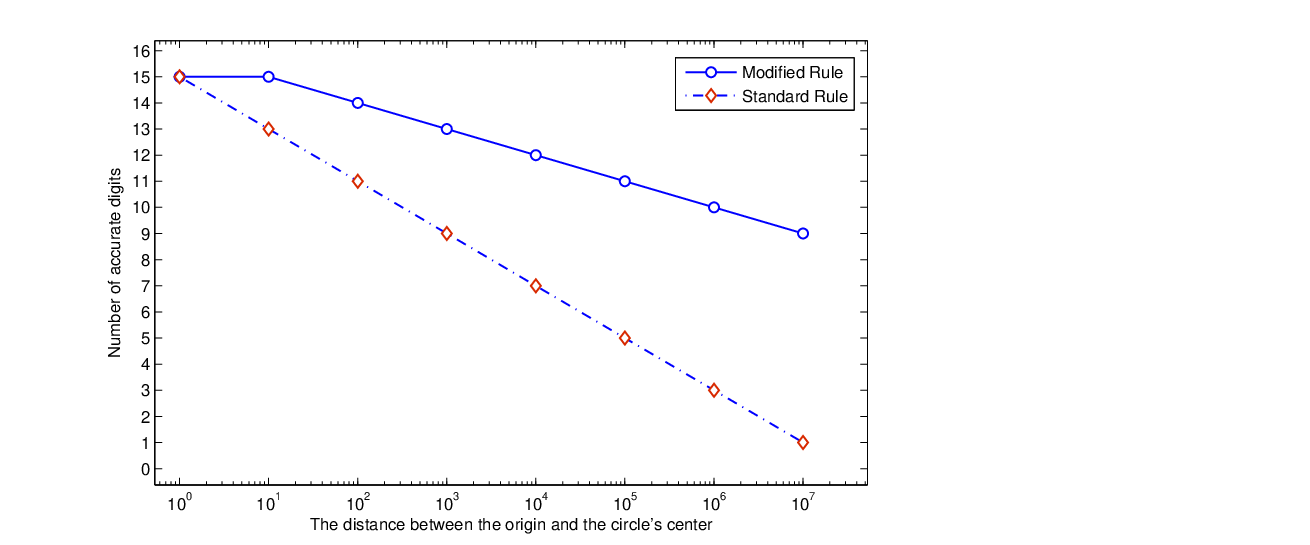
Similar modifications can be made for the formulas (4.1) and (4.2). We omit algebraic details and give the final results. Denote

$$\alpha_{i}=(x_{i}+\gamma_{i}\cos\theta)/w_{i},\qquad\beta_{i}=(y_{i}+\gamma_{i}\sin\theta)/w_{i}$$

$$\eta_{i}=\frac{1}{1+\delta\gamma_{i}},\qquad\kappa_{i}=\frac{\gamma_{i}}{2+\delta\gamma_{i}}$$

Then using our sample mean notation we define

$$P=\tfrac{1}{2}\,(\overline{\tau\gamma\eta}-\delta\,\overline{\tau\gamma\eta\kappa}),\qquad Q=\tfrac{1}{2}\,(\overline{\tau\kappa}+\overline{z})$$

and

$$X=\overline{x\gamma\eta},\qquad Y=\overline{y\gamma\eta}$$

Now the gradient is given by

$$\tfrac{1}{2}\,\nabla\mathcal{F}=\delta\left[\begin{array}[]{c}A\cos\theta-BX\\ A\sin\theta-BY\\ \end{array}\right]$$

(5.2)

where

$$A=P+\delta^{2}(P+Q)Q,\qquad B=1+\delta^{2}Q$$

The Hessian is

$$\tfrac{1}{2}\,\mathcal{H}=\delta^{2}\left[\begin{array}[]{cc}U(2\mathbf{c}-\delta^{2}U)-Q\mathbf{s}^{2}-BN&U\mathbf{s}+V\mathbf{c}-\delta^{2}UV+Q\mathbf{s}\mathbf{c}+BL\\ U\mathbf{s}+V\mathbf{c}-\delta^{2}UV+Q\mathbf{s}\mathbf{c}+BL&V(2\mathbf{s}-\delta^{2}V)-Q\mathbf{c}^{2}-BM\\ \end{array}\right]$$

(5.3)

where we use shorthand notation $\mathbf{c}=\cos\theta$ and $\mathbf{s}=\sin\theta$ and denote

$$U=(P+Q)\mathbf{c}-X,\qquad V=(P+Q)\mathbf{s}-Y$$

and

	$\displaystyle M$	$\displaystyle=(\overline{\gamma\gamma\eta}-Q)\mathbf{c}^{2}+2(\overline{\alpha\gamma\eta}-U)\mathbf{c}+\overline{\alpha\alpha\eta}$
	$\displaystyle N$	$\displaystyle=(\overline{\gamma\gamma\eta}-Q)\mathbf{s}^{2}+2(\overline{\beta\gamma\eta}-V)\mathbf{s}+\overline{\beta\beta\eta}$
	$\displaystyle L$	$\displaystyle=(\overline{\gamma\gamma\eta}-Q)\mathbf{c}\mathbf{s}+(\overline{\alpha\gamma\eta}-U)\mathbf{s}+(\overline{\beta\gamma\eta}-V)\mathbf{c}+\overline{\alpha\beta\eta}$

The above formulas look more complicated than (4.1)–(4.2). Indeed a careful flop count shows that they require $55n+$const flops, while (4.1)–(4.2) require $19n+$const flops, so the computational time roughly triples.

It is shown in [4] that the graph of the objective function $\mathcal{F}(a,b)$ has two valleys stretching toward infinity in opposite directions. In one valley $\mathcal{F}(a,b)$ decreases toward its global minimum, so all the standard algorithms tend to move toward the minimum and converge. The other valley is separated from the minimum by a ridge, and in that valley $\mathcal{F}(a,b)$ decreases as the point $(a,b)$ moves along the valley bottom toward infinity. Thus standard algorithms tend to diverge. We refer to [4, Sec. 3.7] for a detailed account.

To prevent divergence, our program detects whether the current iteration falls in the “wrong” valley, in which case the algorithm restarts from a point in the “right” valley.

The valleys stretch along the eigenvector corresponding to the smaller eigenvalue of the scatter matrix. The latter is given by

$$\mathbf{S}=\left[\begin{array}[]{cc}\overline{xx}&\overline{xy}\\ \overline{xy}&\overline{yy}\\ \end{array}\right]$$

(6.1)

(remember we assumed $\overline{x}=\overline{y}=0$). Now suppose the coordinate system is rotated so that the $x$ direction is aligned with the major eigenvector of $\mathbf{S}$ and the $y$ direction with its minor eigenvector. This gives $\overline{xy}=0$ and $\overline{xx}>\overline{yy}$. Now the valleys stretch in the $y$ (vertical) direction.

Under these conditions it was proven in [4, Sec. 3.9] that the location of the “wrong” valley is determined by the sign of $\overline{xxy}=\frac{1}{n}\sum x_{i}^{2}y_{i}$ as follows:

• (a)

  if $\overline{xxy}>0$, then the wrong valley lies below the $x$ axis;

• (b)

  if $\overline{xxy}<0$, then the wrong valley lies above the $x$ axis.

Our algorithm includes the following block preventing divergence in the wrong valley (here $L>0$ is a large constant; we use $L=100$):

As a restarting point we choose $(0,ZL)$ and rotate it back to the original coordinate system.

Lastly, the best fitting circle may not exist at all [4, 13, 22]. In that case the data points are best fitted by a line (more precisely, by the line passing through the origin and spanned by the major eigenvector of $\mathbf{S}$). It was proven in [4, Sec. 3.9] that this event can only occur if $\overline{xxy}=0$. Thus our algorithm abandons the search for the best circle whenever $\max\{|a|,|b|\}>L$ and $|\overline{xxy}|=O({\boldsymbol{\varepsilon}})$. In that case it returns the best fitting line.

We have compared the proposed algorithm with a few others in a series of computer tests. As competitors, we chose the Gauss-Newton (GN) method described in [8] (the code was downloaded from the author’s web page), the Levenberg-Marquardt (LM) method (see [4, Sec. 4.7]), and the Chernov-Lesort (CL) fit based on algebraic circle parameters (see [6]).

All these fits use the standard stopping rule: they terminate iterations whenever the step gets smaller than ${\boldsymbol{\varepsilon}}^{1/2}$, thus they only achieve suboptimal accuracy $\mathcal{O}({\boldsymbol{\varepsilon}}^{1/2})$. The GN method is actually able to achieve the optimal accuracy $\mathcal{O}({\boldsymbol{\varepsilon}})$ if it continues iterations until the step gets smaller than ${\boldsymbol{\varepsilon}}$. We included this modified version (GNm) in our tests.

In our tests we have generated samples of $n=8$ points randomly, with a uniform distribution in the square $[-1,1]\times[-1,1]$. Each sample was then centered and scaled as described in Section 2. Uniform distribution produced totally “chaotic” samples without any predefined pattern. It is, in a sense, the worst case scenario, corresponding to very large noise in data. Thus our algorithms were tested under the most challenging conditions.

We initialized our fitting algorithms in two different ways. First, we applied a non-iterative algebraic circle fit, such as Kåsa fit [11]. Second, we chose the center $(a,b)$ randomly in the square $[-1,1]\times[-1,1]$ and computed the radius $R$ by (2.1).

Table 1 shows how frequently each algorithm diverges and how many iterations it takes to converge (whenever they do converge). The GN and LM mostly diverge when the iteration gets into the “wrong valley”. The CL fit is designed to converge all the time, but due to its suboptimal accuracy it occasionally stalls. Our results are consistent with the ones reported in [6].

Next we tested the accuracy of each algorithm. For each generated sample we first fitted a very precise circle by using the built-in function vpa (available in MATLAB Symbolic Toolbox) that is able to keep track of 32 (and more) accurate decimal digits. We regard it as “ideal” circle. Now each algorithm produced its own fitting circle and we computed the relative error $E$ in the estimated circle parameters, versus the “ideal” circle. Then we found $k=[-\log_{10}E]$, which is the number of zeros after the decimal point in the digital representation of $E$. This can be roughly interpreted as the number of correct (trustworthy) decimal digits in the parameters of the fitted circle. Whenever $k\geq 15$, the approximation reaches the desired “superaccuracy”. The cases $k\leq 14$ are regarded as “bad enough” to be of interest to us and are recorded.

Table 2 shows the number of recorded “bad” cases for each $k=1,2,...,14$ for each algorithm, after $10^{4}$ runs. The table does not include the super accurate results ($k\geq 15$). All the algorithms here were initialized by the Kåsa algebraic circle fit. We only included runs where all the algorithms converged to the same minimum of the objective function $\mathcal{F}$ (in all these cases $E<10^{-2}$).

The table shows that the methods GN, LM, CL with a suboptimal stopping rule (terminating iterations once the step gets smaller than ${\boldsymbol{\varepsilon}}^{1/2}$) give suboptimal accuracy with $5\leq k\leq 9$ in most cases. The modified GN and our new method use the optimal stopping rule and achieve better accuracy $k\geq 14$ in most cases. But the modified GN falters occasionally having rare bad cases down to $k=4$. And it takes almost 30 iterations, on average to reach the desired accuracy, while our method takes only 8 iterations.

Our numerical results demonstrate the superiority of our new algorithm over the main existing algorithms.

References

- [1] S. J. Ahn, Least Squares Orthogonal Distance Fitting of Curves and Surfaces in Space, LNCS 3151, Springer, Berlin, 2004.
- [2] A. Atieg and G. A. Watson, Fitting circular arcs by orthogonal distance regression, Appl. Numer. Anal. Comput. Math., 1 (2004), 66–76.
- [3] Chan, N. N., 1965. On circular functional relationships, J. R. Statist. Soc. B, 27, 45–56.
- [4] N. Chernov, Circular and linear regression: Fitting circles and lines by least squares, Chapman & Hall/CRC Monographs on Statistics and Applied Probability 117, 2010.
- [5] N. Chernov and C. Lesort, Statistical efficiency of curve fitting algorithms, Comp. Stat. Data Anal., 47 (2004), pp. 713–728.
- [6] N. Chernov and C. Lesort, Least squares fitting of circles, J. Math. Imag. Vision, 23 (2005), 239–251.
- [7] J.F. Crawford, A non-iterative method for fitting circular arcs to measured points, Nucl. Instr. Meth. 211 (1983), 223–225.
- [8] W. Gander, G. H. Golub, and R. Strebel, Least squares fitting of circles and ellipses, BIT, 34 (1994), 558–578.
- [9] S. H. Joseph, Unbiased Least-Squares Fitting Of Circular Arcs, Graph. Models Image Proc. 56 (1994), 424–432.
- [10] V. Karimäki, Effective circle fitting for particle trajectories, Nucl. Instr. Meth. Phys. Res. A 305 (1991), 187–191.
- [11] I. Kasa, A curve fitting procedure and its error analysis, IEEE Trans. Inst. Meas. 25 (1976), 8–14.
- [12] U.M. Landau, Estimation of a circular arc center and its radius, Comp. Vis. Graph. Image Proc. 38 (1987), 317–326.
- [13] Y. Nievergelt, A finite algorithm to fit geometrically all midrange lines, circles, planes, spheres, hyperplanes, and hyperspheres, J. Numerische Math. 91 (2002), 257–303.
- [14] Y. Nievergelt, Perturbation analysis for circles, spheres, and generalized hyperspheres fitted to data by geometric total least-squares, Math. Comp. 73 (2004), 169–180.
- [15] W. H. Press, S. A. Teukolsky, W. T. Vetterling, B. P. Flannery, Numerical Recipes in C++, Cambridge Univ. Press., 2002.
- [16] W. A. Perkins, A model-based vision system for industrial parts, IEEE Trans. Comput. 27 (1978), 126–143.
- [17] C. Shakarji, Least-squares fitting algorithms of the NIST algorithm testing system, J. Res. Nat. Inst. Stand. Techn. 103 (1998), 633–641.
- [18] H. Spath, Least-Squares Fitting By Circles, Computing 57 (1996), 179–185.
- [19] G. Taubin, Estimation Of Planar Curves, Surfaces And Nonplanar Space Curves Defined By Implicit Equations, With Applications To Edge And Range Image Segmentation, IEEE Transactions on Pattern Analysis and Machine Intelligence 13 (1991), 1115–1138.
- [20] L. Trefethen and D. Bau, III, Numerical Linear Algebra, SIAM 1997.
- [21] P. C. Yuen and G. C. Feng, A novel method for parameter estimation of digital arcs, Pattern Recogn. Lett. 17 (1996), 929–938.
- [22] E. Zelniker and V. Clarkson, A statistical analysis of the Delogne-Kåsa method for fitting circles, Digital Signal Proc. 16 (2006), pp. 498–522.