跳到论文正文
W Papers独立论文阅读器 arXiv:1505.03676 论文正文 计算阅读时间 · 0%
引用这篇论文根据当前论文元数据生成,正式投稿前建议核对。


License: arXiv.org perpetual non-exclusive license
arXiv:1505.03676v1 [math.AP] 14 May 2015

Interfaces determined by capillarity and gravity in a two-dimensional porous medium

M. Calle ††thanks: Universidad Carlos III de Madrid (UC3M), Departamento de Economía, Facultad de Ciencias Sociales y Jurídicas, Calle Madrid, 126. 28903 Getafe (Madrid) Spain. E-mail: maria.calle.garcia@uc3m.es    C. M. Cuesta ††thanks: University of the Basque Country (UPV/EHU), Departmento de Matemáticas, Aptdo. 644, 48080 Bilbao, Spain. E-mail: carlotamaria.cuesta@ehu.es    J. J. L. Velázquez ††thanks: Institut für Angewandte Mathematik,Universität Bonn, Endenicher Allee 60, 53115 Bonn, Germany. E-mail: velazquez@iam.uni-bonn.de
Abstract

We consider a two-dimensional model of a porous medium where circular grains are uniformly distributed in a squared container. We assume that such medium is partially filled with water and that the stationary interface separating the water phase from the air phase is described by the balance of capillarity and gravity. Taking the unity as the average distance between grains, we identify four asymptotic regimes that depend on the Bond number and the size of the container. We analyse, in probabilistic terms, the possible global interfaces that can form in each of these regimes. In summary, we show that in the regimes where gravity dominates the probability of configurations of grains allowing solutions close to the horizontal solution is close to one. Moreover, in such regimes where the size of the container is sufficiently large we can describe deviations from the horizontal in probabilistic terms. On the other hand, when capillarity dominates while the size of the container is sufficiently large, we find that the probability of finding interfaces close to the graph of a given smooth curve without self-intersections is close to one.

2010 Mathematics Subject Classification: 35R35, 76S05; 76T10, 76M99, 60C05.

Keywords: capillarity-gravity interface; two-dimensional porous medium; probabilistic asymptotic analysis

1 Introduction

In this paper, we present a two-dimensional model of a porous medium that consists of a squared container partially filled with a liquid and where the pore throats are formed by fixed circular grains that are uniformly distributed. We analyse in probabilistic terms the structure of the stationary interfaces that separate the liquid from air. We consider several parameter regimes where, essentially, either gravity or capillarity dominates.

In this model the form of the interfaces, both at the pore scale and at the macro scale, is determined by the balance between gravity and capillary forces. For a given volume of liquid, these interfaces are the union of single interfaces (see [6]) that meet the solid matrix at given contact angles following Young’s law (see e.g. [1]).

The quasi-stationary system seems to evolve by means of a sequence of local minimizers of the energy. The energy for steady states is the sum of surface energy and potential gravitational energy. The contact angle conditions can be encoded in the different interfacial energies. One of the most relevant features in these flows is the existence of a large number of equilibria that are local minimizers of the total energy of the system. In quasi-stationary situations, if the volume of the liquid phase changes slowly, transitions occur between different minimizers. Understanding the evolution of such a system would require the description of the global motion of the interface that explains the jumps between these multiple local energy minimizers. A first step towards this goal consists in understanding the structure of the minimizers.

The aim of this paper is thus to describe the structure of equilibrium interfaces for different parameter regimes in the model described above. There are several characteristic lengths in the problem, namely, the distance between grains, their size, as well as the macroscopic size of the system. On the other hand, there are other length scales (the capillary length and the inverse of the Bond number) that, as we shall see, give the distances where surface tension and gravity balance (typically, surface tension dominates for small distances and gravity for large ones).

This study is motivated by the experiments presented in Furuberg-Maloy-Feder [11] and [12]. The authors reproduced Haines jumps (see [8]) in a slow drainage process in a container consisting of two plates separated by thin cylinders that act as obstacles or ‘grains’. We recall that Haines jumps are abrupt changes of the pressure in the liquid phase due to sudden changes in the geometry of the interface. From the mathematical point of view these jumps seem to correspond to a fast transition from one equilibrium state to a different one in the capillarity equations.

We mention that there are several mathematical studies related to the study of Multiphase Flow in Porous Media. However, much of the mathematical analysis has focused on the qualitative study of semi-empirical macroscopic descriptions of these flows (see e.g. [2]). There are also rigorous results concerning the derivation of such macroscopic laws from the flows taking place at the pore scale. Not surprisingly, such attends are restricted to single-phase flow (see the chapter of [15], [20]) or simplified models mimicking essential features of multi-phase flow (e.g. [9], [16], [17], [18]). Although our model falls into the second category, we believe that one can analyse simple, but not phenomenological, models in probabilistic terms to get a better understanding of the effect that processes at the pore scale have in the whole system. In this regard, our work is also related to for example [4] (and the references therein), where the propagation of fronts through a random field of obstacles is analysed in relation to hysteresis.

In the next section we set up the mathematical model and discern the parameter regimes under consideration. We outline the contents of the paper at the end of this Introduction.

1.1 The mathematical model and main results

We consider a two dimensional rectangular container of length LL that contains NN uniformly distributed circular grains. If the average distance between grains is d>0d>0 (understood as the average of the distances of every center to its nearest neighbour), then N∝L2/d2N\propto L^{2}/d^{2}. We then let ν>0\nu>0 represent the density of grains, i.e. ν\nu satisfies N=ν​L2/d2N=\nu L^{2}/d^{2}. We assume, for simplicity, that all grains are of equal size and we denote by R<d/2R<d/2 their radius.

The container is partially filled with a liquid so that an interface forms separating the liquid from the air. We assume that such an interface splits the domain in two regions, i.e. it does not intersect itself and there are no isolated bubbles of either of the fluid phases. Let us denote by Γ\Gamma the curve that joins grains and forms the interface, that is the union of capillary(-pressure) curves γ\gamma joining every two grains that meet the interface and that we call elemental components of Γ\Gamma. A sketch of this setting is shown in Figure 1.
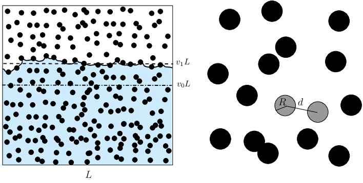
Refer to caption
Figure 1: Schematic picture showing the problem set-up and the three relevant length scales.

Let us fix the canonical basis {𝐞1,𝐞2}\{\mathbf{e}_{1},\mathbf{e}_{2}\} such that 𝐞1=(1,0)\mathbf{e}_{1}=(1,0) and 𝐞2=(0,1)\mathbf{e}_{2}=(0,1), then 𝐞2\mathbf{e}_{2} points in the opposite direction to the gravitational field. We shall denote the coordinates of a point x∈ℝ2x\in\mathbb{R}^{2} by x=(x1,x2)x=(x_{1},x_{2}) in this basis.

Every elemental component of Γ\Gamma, γ\gamma, satisfies the capillary equation (e.g. [6])

σ​H=ρ​g​x2−p,\sigma H=\rho\,gx_{2}-p\,,

that must be complemented with Young’s condition at the grains and/or the walls of the container. We shall assume that the contact angle is the same at all solid surfaces. Here HH denotes the signed curvature of each γ\gamma that forms Γ\Gamma, ρ\rho is the (constant) density of the liquid, gg is the gravity constant and σ\sigma denotes surface tension. Here pp is the pressure associated to the volume fraction of the domain (including grains), v1∈(0,1)v_{1}\in(0,1), occupied by the liquid. Then

p=ρ​g​λwithλ=v1​L.p=\rho\,g\lambda\quad\mbox{with}\quad\lambda=v_{1}L\,.

We take as unit of length the average distance between the grains of the system, dd. Up-scaling the length variables with dd, we obtain that Γ\Gamma satisfies the non-dimensional equation

H=B⁡(x2−λ).H=B\,(x_{2}-\lambda)\,. (1)

subject to a contact angle boundary condition that we specify below. We obtain the non-dimensional number BB, which is the Bond number

B=ρ​g​d2σ,B=\frac{\rho gd^{2}}{\sigma}\,, (2)

and measures the balance between gravitational forces and surface tension in this units of length.

For simplicity, we use the same notation for the non-dimensional variables. Also we let LL and RR be the non-dimensional size of the domain (i.e. L/dL/d) and grain radius (i.e. R/dR/d), respectively. This, in particular, means that, with this notation, λ=v1​L\lambda=v_{1}L in (1). We observe that v1v_{1} depends on the configuration of grains, so if we let v0∈[0,1]v_{0}\in[0,1] be the volume fraction of the domain occupied by the liquid, the volume occupied by the liquid is v0​L2v_{0}L^{2} and then

v1​L2≈v0​L2+n​π​R2v_{1}L^{2}\approx v_{0}L^{2}+n\pi R^{2} (3)

is the volume below the interface Γ\Gamma, if nn is the number of grains below Γ\Gamma.

We assume thereafter that v0v_{0} is fixed, and we take the horizontal line x2=v1​Lx_{2}=v_{1}L(=λ=\lambda) as a reference height for each configuration of grains. Observe that this is a solution of (1) with α=0\alpha=0 at the walls.

We also observe that with the new notation, where LL and RR are non-dimensional lengths, then the number of grains in the container is N=ν​L2N=\nu L^{2}. Henceforth, with this scaling we can think of the equivalent problem where the liquid and air occupy some space in a square domain [0,L]2[0,L]^{2} with L≫1L\gg 1, where ν​L2\nu L^{2} grains are uniformly distributed with an average distance 11 between them.

We indicate the position of a center by the variable ξ=(ξ(1),ξ(2))∈ℝ2\xi=(\xi^{(1)},\xi^{(2)})\in\mathbb{R}^{2} and write its boundary in the form ∂BR​(ξ)\partial B_{R}(\xi). We take 𝐧\mathbf{n} as the unit normal vector to Γ\Gamma pointing in the direction of air, and 𝐭\mathbf{t} the tangent vector to Γ\Gamma such that {𝐭,𝐧}\{\mathbf{t},\mathbf{n}\} has the same orientation as the canonical basis (i.e. that det(𝐭,𝐧)=1\det(\mathbf{t},\mathbf{n})=1).

Let us denote by 𝐍\mathbf{N} the outer normal vector to ∂BR​(ξ)\partial B_{R}(\xi) at a point PP where Γ\Gamma and ∂BR​(ξ)\partial B_{R}(\xi) intersect (i.e. PP is a contact point). Let us denote by 𝐭c\mathbf{t}_{c} the value of 𝐭\mathbf{t} at PP. Then, the Young condition is defined as follows: if 𝐍⋅𝐭c≥𝟎\mathbf{N}\cdot\mathbf{t}_{c}\mathbf{\geq 0},

𝐍∧𝐭c=sin⁡(α)​𝐞3\mathbf{N}\wedge\mathbf{t}_{c}=\sin(\alpha)\mathbf{e}_{3} (4)

where α∈[−π2,π2]\alpha\in\left[-\frac{\pi}{2},\frac{\pi}{2}\right] is the contact angle and where 𝐞3=𝐞1∧𝐞2\mathbf{e}_{3}=\mathbf{e}_{1}\wedge\mathbf{e}_{2}. If 𝐍⋅𝐭c<0\mathbf{N}\cdot\mathbf{t}_{c}<0, then with the same choice of 𝐞1\mathbf{e}_{1}, we set 𝐍∧𝐭c=sin⁡(α−π)​𝐞3\mathbf{N}\wedge\mathbf{t}_{c}=\sin(\alpha-\pi)\mathbf{e}_{3}.

We shall distinguish different parameter regimes. The following observations are then in order. We recall that BB is the Bond number with respect to the scale given by the distance between grains. In the case B≫1B\gg 1 the gravitational effects are the dominant ones. In this limit the liquid-gas interfaces tend to be horizontal lines, corrected by boundary layers of height 1/B1/\sqrt{B}. In the limit B≪1B\ll 1, the interfaces are dominated by surface tension and this allows vertical variations in the connection between grains (of the order of the distance between the grains). Thus, unlike in the case B≫1B\gg 1, if B≪1B\ll 1 the connections can take place in any direction, not just horizontally.

The above regimes take into account the size of BB only, but we shall relate it to LL as well. In particular, the limit L→∞L\to\infty gives an ever increasing number of grains and can in principle give rise to ’anomalous’ situations (not sketched above) that we analyse in detail in Section 3 and that we summarise below.

We distinguish several cases depending on the relative size of BB and LL. In the cases where B≫1B\gg 1, we actually compare LL to min⁡{B,R−1}\min\{\sqrt{B},R^{-1}\}, which relates the height of the boundary layers to RR:

  1. (i)

    The regime 1≲L≪min⁡{B,R−1}1\lesssim L\ll\min\{\sqrt{B},R^{-1}\}, where B→∞B\to\infty and R→0R\to 0 (Section 3.1 Theorem 3.3): In this case gravity dominates and the size of the container is not sufficiently large to allow significant capillarity effects. We find that as B→∞B\to\infty there are configurations with probability close to 11 for which the solution interfaces tend to the horizontal solution. One can in fact distinguish the cases L=O⁡(1)L=O(1) and L→∞L\to\infty, with either R≪1/BR\ll 1/\sqrt{B} or R≫1/BR\gg 1/\sqrt{B}, with the same result.

  2. (ii)

    The regime L=O⁡(min⁡{B,R−1})L=O(\min\{\sqrt{B},R^{-1}\}) and L→∞L\to\infty (Section 3.2 Theorem 3.5): In this case we find that the probability of finding solutions close to the horizontal line is close to one. On the other hand we also find that the probability of finding configurations that have a given number of elemental components is close to zero, but bounded from above by a Poisson distribution. Again, the distinction between the cases 1/B≫R1/\sqrt{B}\gg R and 1/B≪R1/\sqrt{B}\ll R is not significant.

  3. (iii)

    The regime L≫min⁡{B,R−1}L\gg\min\{\sqrt{B},R^{-1}\} and L→∞L\to\infty:

    1. (a)

      The case B→∞B\to\infty (and R→0R\to 0) (Section 3.3 Theorem 3.10). This is a regime where gravity in principle dominates, we find an interval of LL in terms of BB where with probability close to one solutions stay in a narrow strip around the horizontal reference line. For LL above this range there is no guarantee that solutions are necessarily close to the horizontal reference line. If 1/B≫R1/\sqrt{B}\gg R, the interval is B≪L≪B​log⁡(B)\sqrt{B}\ll L\ll\sqrt{B}\log(B), and if 1/B≪R1/\sqrt{B}\ll R with R→0R\to 0, the result holds replacing 1/B1/\sqrt{B} by RR.

    2. (b)

      The case B=O⁡(1)B=O(1). In this case, capillary and gravity forces are comparable and it is not possible to derive general properties about the structure of the solution interfaces using perturbative methods. Therefore this regime is not included in our analysis.

    3. (c)

      The case B→0B\to 0 (Section 3.4 Theorem 3.12). We will see that in this case the only meaningful limit is that of L=O⁡(1/B)L=O(1/B). When B→0B\to 0, the maximum fluctuation of height of a solution Γ\Gamma are of the order of 1/B1/B. In this regime, we can show that with probability close to one, we can find interfaces that are suitably close to any smooth curve without self-intersections that connect (following its orientation) {0}×[0,L]\{0\}\times[0,L] to {L}×[0,L]\{L\}\times[0,L].

In order to understand the probabilistic problem we need to analyse the elemental components that an interface Γ\Gamma can have. This is done in Section 2 where we analyse the solution curves of (1) and characterise them in terms of a free parameter that controls the height reached by the curve and its curvature. In fact, equation (1) implies that the curvature of an elemental component increases in absolute value with the distance to the reference height. The main results and their proofs are presented in Section 3, where the regimes outlined above are studied separately. Finally, Appendix A deals with the proof of a technical lemma that is needed in Section 3.3.

2 Preliminary Analysis: Gluing of Solutions

In this section we analyse the basic features of elemental components of an interface Γ\Gamma. We first observe that equation (1) in the absence of boundary conditions can be solved explicitly in terms of elliptic integrals, see [13]. One can achieve this by first introducing the variable x¯2=x2−λ\bar{x}_{2}=x_{2}-\lambda and using the angle β∈[−π,π]\beta\in[-\pi,\pi] from 𝐞1\mathbf{e}_{1} to the tangent vector 𝐭=(x1′​(s),x¯2′​(s))\mathbf{t}=(x_{1}^{\prime}(s),\bar{x}_{2}^{\prime}(s)) where ss is the arc-length. Then multiplying (1) by x¯2′​(s)\bar{x}_{2}^{\prime}(s) and integrating once we get

B​x¯222+cos⁡β=C,B\frac{\bar{x}_{2}^{2}}{2}+\cos\beta=C\,, (5)

where CC is a constant of integration that can have either sign or be zero, but clearly C≥−1C\geq-1. Then solving (1), with given initial conditions, amounts to solving

x1′​(s)=cos⁡βx¯2′​(s)=sin⁡βx_{1}^{\prime}(s)=\cos\beta\quad\bar{x}_{2}^{\prime}(s)=\sin\beta (6)

subject to the same initial conditions, together with (5) and a compatible constant CC.

The are the obvious symmetries of equation (1), (x1,s)→(2​a−x1,−s)(x_{1},s)\rightarrow(2a-x_{1},-s) (for any a∈ℝa\in\mathbb{R}) and x¯2→−x¯2\bar{x}_{2}\rightarrow-\bar{x}_{2}, that will be used to simplify the computations below.

Using (6) and the definition of arc-length, one can write (5) as

[1−(C−B​x¯222)2]​(d​x1)2=(C−B​x¯222)2​(d​x¯2)2\left[1-\left(C-B\frac{\bar{x}_{2}^{2}}{2}\right)^{2}\right]\left(dx_{1}\right)^{2}=\left(C-B\frac{\bar{x}_{2}^{2}}{2}\right)^{2}\left(d\bar{x}_{2}\right)^{2} (7)

The fact that we are taking squares to go from (1) to (7) means that the set of solutions of the latter is larger than that of the former. In the construction one has to impose that the resulting curves are indeed solutions of (1), as we shall see. We also notice that all solutions must have |x¯2|≤2​(C+1)/B|\bar{x}_{2}|\leq\sqrt{2(C+1)/B}.

Below, we find the solutions of (1) by gluing together pieces of curve solutions that are graphs of a function of the form x1​(x¯2)x_{1}(\bar{x}_{2}) and that solve (7). We then integrate (7) after taking the positive or negative square root of (d​x1)2/(d​x¯2)2(dx_{1})^{2}/(d\bar{x}_{2})^{2}; we use the equations:

d​x1d​x¯2=±C−B​x¯2221−(C−B​x¯222)2.\frac{dx_{1}}{d\bar{x}_{2}}=\pm\frac{C-B\displaystyle{\frac{\bar{x}_{2}^{2}}{2}}}{\sqrt{1-\left(C-B\displaystyle{\frac{\bar{x}_{2}^{2}}{2}}\right)^{2}}}\,. (8)

Observe that β\beta, for such graphs, is characterised by

d​x1d​x¯2=1tan⁡β.\frac{dx_{1}}{d\bar{x}_{2}}=\frac{1}{\tan\beta}\,.

There are solutions, however, that cannot be constructed the way explained above. These are the solutions with x¯2≡0\bar{x}_{2}\equiv 0, that is the curves (s,0)(s,0) (air is on top of the liquid) and (−s,0)(-s,0) (air is below the liquid). The former corresponds to a solution of (5) with C=1C=1, and the latter to a solution of (5) with C=−1C=-1.

Next, we identify the points of the solution curves where either x1′​(s)=0x_{1}^{\prime}(s)=0 or x¯2′​(s)=0\bar{x}_{2}^{\prime}(s)=0, i.e. the values of x¯2\bar{x}_{2} where either the left or the right-hand side of (7) vanishes. For simplicity, we use the following notation:

x2m​i​n​(C,B):={2​(C−1)BifC>10otherwisex_{2}^{min}(C;B):=\left\{\begin{array}[]{l}\displaystyle{\sqrt{\frac{2(C-1)}{B}}}\quad\mbox{if}\quad C>1\\ 0\quad\mbox{otherwise}\end{array}\right. (9)

and

x2m​e​d​(C,B):=2​CB,x2m​a​x​(C,B):=2​(C+1)Bx_{2}^{med}(C;B):=\sqrt{\frac{2C}{B}}\,,\quad x_{2}^{max}(C;B):=\sqrt{\frac{2(C+1)}{B}} (10)
Lemma 2.1

The points at which either x1′​(s)=0x_{1}^{\prime}(s)=0 or x¯2′​(s)=0\bar{x}_{2}^{\prime}(s)=0 are as follows:

  1. (i)

    If C≥0C\geq 0, when x1′​(s)=0x_{1}^{\prime}(s)=0 then x¯2=±x2m​e​d​(C,B)\bar{x}_{2}=\pm x_{2}^{med}(C;B), and when x2′​(s)=0x_{2}^{\prime}(s)=0 then either x¯2=±x2m​i​n​(C,B)\bar{x}_{2}=\pm x_{2}^{min}(C;B) or x¯2=±x2m​a​x​(C,B)\bar{x}_{2}=\pm x_{2}^{max}(C;B), except if 0≤C<10\leq C<1, that x2′​(s)=0x_{2}^{\prime}(s)=0 only occurs at x¯2=±x2m​a​x​(C,B)\bar{x}_{2}=\pm x_{2}^{max}(C;B).

  2. (ii)

    If C<0C<0, then there is no value of ss such that x1′​(s)=0x_{1}^{\prime}(s)=0, and as before, x2′​(s)=0x_{2}^{\prime}(s)=0 occurs at x¯2=±x2m​a​x​(C,B)\bar{x}_{2}=\pm x_{2}^{max}(C;B).

The next lemma describes the way solutions of (1) can be obtained by gluing solutions of (the branch equations) (8) at points with either vertical or horizontal tangent vector.

Lemma 2.2 (Gluing rule)

For C>−1C>-1, given the initial condition (x1​(0),x¯2​(0))=(a,x2m​a​x​(C,B))(x_{1}(0),\bar{x}_{2}(0))=(a,x_{2}^{max}(C;B)) with a∈ℝa\in\mathbb{R} and (x1′​(0),x¯2′​(0))=(−1,0)(x_{1}^{\prime}(0),\bar{x}_{2}^{\prime}(0))=(-1,0) for (1), this specifies the branch equation of (8) that the corresponding solution (1) satisfies. If this solution reaches a point with x1′​(s)=0x_{1}^{\prime}(s)=0 then it can only be continued further by solving the same branch of (8). On the other hand, if the curve reaches a point with x¯2′​(s)=0\bar{x}_{2}^{\prime}(s)=0 then it can only be continued further by solving the branch equation with opposite sign.

Proof. A solution stops being a graph of a function of the form x1​(x¯2)x_{1}(\bar{x}_{2}) when, seen as a curve, x¯2′​(s)=0\bar{x}_{2}^{\prime}(s)=0. It is easy to see that, this never occurs at a point with x¯2=0\bar{x}_{2}=0. At those points we can further continue the solution curve by gluing smoothly with another solution curve that solves (8) with the opposite sign (notice that these curves, as graphs, have the opposite orientation, and hence the change of sign in (8) implies that they have the same curvature at that point).

On the other hand, at points with x1′​(s)=0x_{1}^{\prime}(s)=0, the solution is still a graph, and in principle, one could glue it to a solution that solves (8) with the opposite sign. However, if this happens at a point with x¯2≠0\bar{x}_{2}\neq 0, then HH would change sign, which contradicts (1). If, this happens at a point with x¯2=0\bar{x}_{2}=0, then HH keeps its sign, but this also contradicts (1).  

We now construct pieces of curve solutions from which one can recover complete solutions of (1) (i.e. defined for all s∈ℝs\in\mathbb{R}) by the symmetries (x1,s)→(2​a−x1,−s)(x_{1},s)\to(2a-x_{1},-s), for any a∈ℝa\in\mathbb{R}, and x¯2→−x¯2\bar{x}_{2}\to-\bar{x}_{2}. The next lemma gives these pieces for every C>−1C>-1 by distinguishing the cases C>1C>1, 1>C>01>C>0 and 0≥C>−10\geq C>-1.

Lemma 2.3 (The pieces)

Given the initial condition (x1​(0),x¯2​(0))=(a,x2m​a​x​(C,B)𝐶𝐿𝑂𝑆𝐸(x_{1}(0),\bar{x}_{2}(0))=(a,x_{2}^{max}(C;B), with C>−1C>-1 and a∈ℝa\in\mathbb{R}, and (x1′​(0),x¯2′​(0))=(−1,0)(x_{1}^{\prime}(0),\bar{x}_{2}^{\prime}(0))=(-1,0) for (1), the elemental component of the solution curve is obtained by integrating (8), with the minus sign, up to a x¯2=0\bar{x}_{2}=0 or up to x¯2=x2m​i​n​(C,B)\bar{x}_{2}=x_{2}^{min}(C;B). Namely,

  1. (i)

    For C>1C>1, the curve starts with d​x1/d​x¯2≥0dx_{1}/d\bar{x}_{2}\geq 0 and reaches x¯2=x2m​e​d​(C,B)\bar{x}_{2}=x_{2}^{med}(C;B) for some value of ss, for which x1′​(s)=0x_{1}^{\prime}(s)=0 and x¯2′​(s)=−1\bar{x}_{2}^{\prime}(s)=-1. The curve continues with d​x1/d​x¯2≤0dx_{1}/d\bar{x}_{2}\leq 0  up to a point where x¯2=x2m​i​n​(C,B)>0\bar{x}_{2}=x_{2}^{min}(C;B)>0 for some other value of ss, for which x1′​(s)=1x_{1}^{\prime}(s)=1 and x¯2′​(s)=0\bar{x}_{2}^{\prime}(s)=0.

  2. (ii)

    For C=1C=1, the curve starts with d​x1/d​x¯2≥0dx_{1}/d\bar{x}_{2}\geq 0 and reaches x¯2=2B\bar{x}_{2}=\sqrt{\frac{2}{B}}, for which x1′​(s)=0x_{1}^{\prime}(s)=0 and x¯2′​(s)=−1\bar{x}_{2}^{\prime}(s)=-1. The curve continues with d​x1/d​x¯2≤0dx_{1}/d\bar{x}_{2}\leq 0 and has an asymptote at x¯2=0\bar{x}_{2}=0, that is with x1​(s)→∞x_{1}(s)\to\infty and x¯2​(s)→0+\bar{x}_{2}(s)\to 0^{+} as s→∞s\to\infty.

  3. (iii)

    For 0<C<10<C<1, the curve starts with d​x1/d​x¯2≥0dx_{1}/d\bar{x}_{2}\geq 0 and reaches x¯2=x2m​e​d​(C,B)\bar{x}_{2}=x_{2}^{med}(C;B) at some value of ss, for which x1′​(s)=0x_{1}^{\prime}(s)=0 and x¯2′​(s)=−1\bar{x}_{2}^{\prime}(s)=-1. The curve continues with d​x1/d​x¯2≤0dx_{1}/d\bar{x}_{2}\leq 0  up to a point where x¯2=0\bar{x}_{2}=0 at some other value of ss, for which x1′​(s)>0x_{1}^{\prime}(s)>0 and x¯2′​(s)<0\bar{x}_{2}^{\prime}(s)<0.

  4. (iv)

    For −1<C≤0-1<C\leq 0, the curve starts with d​x1/d​x¯2≥0dx_{1}/d\bar{x}_{2}\geq 0 and reaches x¯2=0\bar{x}_{2}=0 at some value of ss, for which x1′​(s)=0x_{1}^{\prime}(s)=0 and x¯2′​(s)=−1\bar{x}_{2}^{\prime}(s)=-1, if C=0C=0, and x1′​(s)<0x_{1}^{\prime}(s)<0 and x¯2′​(s)<0\bar{x}_{2}^{\prime}(s)<0, otherwise.

Proof. We only prove (i), thus, let us assume that C>1C>1. We first observe that due to the fact that the maximum value that x¯2\bar{x}_{2} can take is the initial one, the direction of the initial tangent vector implies that away from, but close to, the initial point d​x1/d​x¯2>0dx_{1}/d\bar{x}_{2}>0. Then the curve solution can be seen as a graph of a function of the form x1​(x¯2)x_{1}(\bar{x}_{2}) that solves (8) with the minus sign. Then the solution x1​(x¯2)x_{1}(\bar{x}_{2}) is convex as long as x¯2∈(x2m​i​n​(C,B),x2m​a​x​(C,B))\bar{x}_{2}\in(x_{2}^{min}(C;B),x_{2}^{max}(C;B)) (see (1), that implies sign​(d2​x1/d​x¯22)=sign​(x¯2)\mbox{sign}(d^{2}x_{1}/d\bar{x}_{2}^{2})=\mbox{sign}(\bar{x}_{2})). In particular, this curve reaches a point with x¯2=x2m​e​d​(C,B)\bar{x}_{2}=x_{2}^{med}(C;B) (i.e. with (x1′​(s),x¯2′​(s))=(0,−1)(x_{1}^{\prime}(s),\bar{x}_{2}^{\prime}(s))=(0,-1) for some value of ss). In order to prove that the curve also reaches a point with x¯2=x2m​i​n​(C,B)\bar{x}_{2}=x_{2}^{min}(C;B) (i.e. with (x1′​(s),x¯2′​(s))=(1,0)(x_{1}^{\prime}(s),\bar{x}_{2}^{\prime}(s))=(1,0) for some value of ss), we construct a curve ending up at such a point, and by a similar argument this curve also passes through a point with x¯2=x2m​e​d​(C,B)\bar{x}_{2}=x_{2}^{med}(C;B). Then, adjusting the initial value of x1x_{1} so that both curves intersect at such a point (which they do tangentially), and using the uniqueness provided by Lemma 2.2 imply that they are the same solution curve.

All the other cases are straight forward by convexity of the solution curve.  

We show in figures 2(a) (for C>1C>1), 2(b) (for 0<C<10<C<1),  3 (for C=1C=1),  2(c) (for C=0C=0) and  2(d) (for −1<C<0-1<C<0) the pieces described in Lemma 2.3. The next lemma describes how complete curves are obtained from these pieces.


Refer to caption
(a) C>1C>1
Refer to caption
(b) 0<C<10<C<1
Refer to caption
(c) C=0C=0
Refer to caption
(d) −1<C<0-1<C<0
Figure 2: This picture shows solution curves of (5) with C>0C>0 and C≠1C\neq 1. The dashed-dotted line represents the line x¯2=0\bar{x}_{2}=0, and the dashed horizontal ones are the lines x¯2=±x2m​a​x​(C,B)\bar{x}_{2}=\pm x_{2}^{max}(C;B). The thick solid lines represent the pieces of curves as specified in Lemma 2.3. The remaining lines give solutions obtained by the symmetries x¯2→−x¯2\bar{x}_{2}\to-\bar{x}_{2} and x1→−x1x_{1}\to-x_{1}, see Lemma 2.4. Any other solution is a translation of the ones shown. Complete solutions curves to (1) are achieved by the smooth gluing of these ones at the points with x¯2′​(s)=0\bar{x}_{2}^{\prime}(s)=0 on the dashed lines. 2(a) shows the case C>1C>1 and 2(b) shows the case in which 0<C<10<C<1. According to the orientation shown in these cases the air lies ‘on top’ of the graphs shown. 2(c) shows the case C=01C=01 and 2(d) shows the case in which −1<C<0-1<C<0. In these cases, the air lies below the graphs.
Lemma 2.4 (Complete curve solutions)

For each C>−1C>-1, the pieces of solution curves obtained in Lemma 2.3 give rise to complete curves, as follows:

  1. (i)

    There are three additional pieces of curve solutions obtained by the symmetries x1→−x1x_{1}\to-x_{1} and x¯2→−x¯2\bar{x}_{2}\to-\bar{x}_{2}.

  2. (ii)

    In all cases above the curves obtained can be glued together smoothly, translating as necessary in x1x_{1}, at the points where x¯2′​(s)=0\bar{x}_{2}^{\prime}(s)=0, and at points with x¯2=0\bar{x}_{2}=0 (choosing pieces with the same tangent vector at the point).

Remark 2.5
  1. (i)

    The complete curves that we obtain are open and periodic except for a particular value of CC for which the complete curves are closed: by continuity, there exists a value of C∈(0,1)C\in(0,1), say C0C_{0} (actually C0≈0.6522C_{0}\approx 0.6522, see [13]), such that the corresponding elemental component satisfies that x1​(0)=x1​(x2m​a​x​(C,B))x_{1}(0)=x_{1}\left(x_{2}^{max}(C;B)\right). In particular, if C>C0C>C_{0}, the curve obtained in Lemma 2.4 has, globally, increasing x1x_{1} as s→∞s\to\infty, whereas the corresponding curve if C<C0C<C_{0} has, globally, decreasing x1x_{1} as s→∞s\to\infty.

    Physically, one can interpret the solution curves with C<C0C<C_{0} as describing a situation in which air lies below the liquid, and vice versa for the ones with C>C0C>C_{0}.

  2. (ii)

    It is also worth mentioning that the complete curve obtained for C∈(−1,0]C\in(-1,0] that oscillates around x¯2=0\bar{x}_{2}=0 does not have self-intersections and can in principle connect two grains very far apart (in the horizontal direction).

The next lemma gives the range of β\beta that complete curve have depending on CC:

Lemma 2.6 (Range of β\beta)

For the complete curves obtained in Lemma 2.4 the values of the angle β\beta range in different intervals depending on CC:

  1. (i)

    If C>1C>1, β\beta takes all values in [−π,π][-\pi,\pi].

  2. (ii)

    If C=1C=1, β\beta takes all values in [−π,0)∪(0,π][-\pi,0)\cup(0,\pi], unless the solution is the horizontal line, for which β≡0\beta\equiv 0.

  3. (iii)

    If −1≤C<1-1\leq C<1, β\beta takes all values in [−π,−η]∪[η,π][-\pi,-\eta]\cup[\eta,\pi] for some η∈(0,π]\eta\in(0,\pi], and η\eta increases when CC decreases (in fact, η=π\eta=\pi if and only if C=−1C=-1, i.e. x¯2≡0\bar{x}_{2}\equiv 0 with 𝐧\mathbf{n} pointing in the direction of gravity, and η=π/2\eta=\pi/2 if and only if C=0C=0).

Remark 2.7
  1. (i)

    We observe that by the determination of β\beta that we have chosen, its value jumps from π\pi to −π-\pi at gluing points with x¯2=x2m​a​x​(C,B)\bar{x}_{2}=x_{2}^{max}(C;B), and, similarly, its value jumps from −π-\pi to π\pi at gluing points with x¯2=−x2m​a​x​(C,B)\bar{x}_{2}=-x_{2}^{max}(C;B).

  2. (ii)

    We observe that given the contact angle α\alpha and the radius of grains RR, the contact point at a grain is given by the angle ρc\rho_{c} measured from the horizontal placed at the center of the grain to the contact point, and satisfies

    ρc=α−βc\rho_{c}=\alpha-\beta_{c} (11)

    where βc\beta_{c} is β\beta at the contact point.

    Then Lemma 2.6 gives the possible range of ρc\rho_{c} for a given α\alpha· In particular, if C≥1C\geq 1 ρc\rho_{c} covers one period and unique solution exists between two given grains that are sufficiently close by adjusting CC. If −1≤C<1-1\leq C<1, then ρc∈[α−π,α−η]∪[α+η,α+π]\rho_{c}\in[\alpha-\pi,\alpha-\eta]\cup[\alpha+\eta,\alpha+\pi]. This means that there are some restrictions on the contact surface ∂BR​(ξ)\partial B_{R}(\xi) for grains that lie near the horizontal if air lies below the interface.

We give the solutions of (5) with C=1C=1 explicitly in the next lemma, see also Figure 3

Refer to caption

Figure 3: This picture shows four solution branches of (5) with C=1C=1. One if then is, in this case, x¯2≡0\bar{x}_{2}\equiv 0 (dashed-dotted line). The complete solution curves to (1) are achieved by smoothly gluing at x¯2=x2m​e​d​(C,B)\bar{x}_{2}=x_{2}^{med}(C;B) or at x¯2=−x2m​e​d​(C,B)\bar{x}_{2}=-x_{2}^{med}(C;B) (dashed line), depending on the sign, and translating in the direction of x1x_{1} copies of the ones shown.
Lemma 2.8

The solutions of (5) with C=1C=1 are explicitly given by the horizontal line x¯2≡0\bar{x}_{2}\equiv 0 oriented with 𝐧=𝐞2\mathbf{n}=\mathbf{e}_{2}, and by two one-parameter families of solution branches:

x1+​(x¯2,a)=−1B​F​(B​x¯2)+a,x¯2∈(−2B,0)∪(0,2B),x_{1}^{+}(\bar{x}_{2};a)=-\frac{1}{\sqrt{B}}F(\sqrt{B}\bar{x}_{2})+a,\;\;\bar{x}_{2}\in\left(-\frac{2}{\sqrt{B}},0\right)\cup\left(0,\frac{2}{\sqrt{B}}\right),
x1−​(x¯2,a)=1B​F​(B​x¯2)+a,x¯2∈(−2B,0)∪(0,2B),x_{1}^{-}(\bar{x}_{2};a)=\frac{1}{\sqrt{B}}F(\sqrt{B}\bar{x}_{2})+a,\;\;\bar{x}_{2}\in\left(-\frac{2}{\sqrt{B}},0\right)\cup\left(0,\frac{2}{\sqrt{B}}\right)\,,

where the parameter aa is a real number and FF is given by

F⁡(Z)=12​log⁡(2−4−Z22+4−Z2)+4−Z2,Z∈(−2,0)∪(0,2).F(Z)=\frac{1}{2}\log\left(\frac{2-\sqrt{4-Z^{2}}}{2+\sqrt{4-Z^{2}}}\right)+\sqrt{4-Z^{2}},\;Z\in(-2,0)\cup(0,2)\,. (12)

Moreover, FF satisfies the following properties: limZ→−2+F⁡(Z)=limZ→2−F⁡(Z)=0\lim_{Z\to-2^{+}}F(Z)=\lim_{Z\to 2^{-}}F(Z)=0 and limZ→0±F⁡(Z)=−∞\lim_{Z\to 0^{\pm}}F(Z)=-\infty. Observe also that F′​(Z)=0F^{\prime}(Z)=0 at Z=±2Z=\pm\sqrt{2} and that limZ→−2+F′​(Z)=∞\lim_{Z\to-2^{+}}F^{\prime}(Z)=\infty, limZ→2−F′​(Z)=−∞\lim_{Z\to 2^{-}}F^{\prime}(Z)=-\infty and limZ→0±F′​(Z)=±∞\lim_{Z\to 0^{\pm}}F^{\prime}(Z)=\pm\infty. Regarding convexity; F′′​(Z)<0F^{\prime\prime}(Z)<0 with Z∈(−2,0)∪(0,2)Z\in(-2,0)\cup(0,2).

Remark 2.9
  1. (i)

    We notice that the functions x1+x_{1}^{+} and x1−x_{1}^{-} can be extended to x¯2=±2/B\bar{x}_{2}=\pm 2/\sqrt{B}, with x1+(±2/B;a)=ax_{1}^{+}(\pm 2/\sqrt{B};a)=a and x1−(±2/B;a)=ax_{1}^{-}(\pm 2/\sqrt{B};a)=a, but the derivative at those points is not finite. We also observe that gluing together the branch x1+x_{1}^{+} and x1−x_{1}^{-} with x¯2∈[−2/B,0)\bar{x}_{2}\in[-2/\sqrt{B},0), and the same value of aa we obtain a complete planar curve. Similarly, x1+x_{1}^{+} and x1−x_{1}^{-} with x¯2∈(0,2/B]\bar{x}_{2}\in(0,2/\sqrt{B}] for the same aa give another complete curve, that can be simply recovered from the previous one by the transformation x¯2→−x¯2\bar{x}_{2}\to-\bar{x}_{2}.

  2. (ii)

    We observe that the limit C→1C\to 1 can be studied independently of the value of BB. One can easily show that solutions with positive CC, and either C>1C>1 or C<1C<1 converge to the solutions found in Lemma 2.8 on compact sets of x2x_{2}.

The rest of the section is devoted to deriving estimates on the maximal horizontal length of a solution curve depending on the value of CC. First we derive the horizontal length at points where the height is minimum or 00 to points where the height is x2m​e​dx_{2}^{med} or x2m​a​xx_{2}^{max}:

Lemma 2.10

Given a elemental component solution as in Lemma 2.3:

  1. (i)

    If −1<C≤0-1<C\leq 0, then

    log⁡(2+21+3)​1B<x1​(x2m​a​x​(C,B))−x1​(0)<π2​B.\log\left(\frac{2+\sqrt{2}}{1+\sqrt{3}}\right)\frac{1}{\sqrt{B}}<x_{1}(x_{2}^{max}(C;B))-x_{1}(0)<\frac{\pi}{\sqrt{2B}}\,.
  2. (ii)

    If 0<C<10<C<1, then

    1B​h1​(C)<x1​(0)−x1​(x2m​e​d​(C,B))<1B​h2​(C).\frac{1}{\sqrt{B}}h_{1}(C)<x_{1}(0)-x_{1}\left(x_{2}^{med}(C;B)\right)<\frac{1}{\sqrt{B}}h_{2}(C)\,.

    where hi​(C)→0h_{i}(C)\to 0 as C→0C\to 0 and hi​(C)=O⁡(−log⁡(1−C))h_{i}(C)=O(-\log(\sqrt{1-C})) as C→1−C\to 1^{-}, for both i=1,2i=1,2.

  3. (iii)

    If C>1C>1, then there exist non-negative functions h3​(C)h_{3}(C) and h4​(C)h_{4}(C), continuous in CC, such that,

    1B​h3​(C)<x1​(x2m​i​n​(C,B))−x1​(x2m​e​d​(C,B))<1B​h4​(C),\frac{1}{\sqrt{B}}h_{3}(C)<x_{1}\left(x_{2}^{min}(C;B)\right)-x_{1}\left(x_{2}^{med}(C;B)\right)<\frac{1}{\sqrt{B}}h_{4}(C)\,,

    where OPENhi​(C)=O⁡(−log⁡C−1))h_{i}(C)=O(-\log\sqrt{C-1})) as C→1+C\to 1^{+}, for both i=3,4i=3,4 and hi​(C)=O⁡(1/C)h_{i}(C)=O(1/\sqrt{C}) as C→∞C\to\infty, for both i=3,4i=3,4.

Proof. In order to prove the estimates we use Lemma 2.3 and integrate (8) over x¯2\bar{x}_{2} in the appropriate interval where x1​(x¯2)x_{1}(\bar{x}_{2}) is monotone. Then we estimate the integrand (that is the right-hand side of (8)) with the minus sign by using straightforward bounds on the numerator and on the denominator. Namely, we estimate the parabola C−B​Z22C-B\frac{Z^{2}}{2} from above and below. We also write (1−(C−B​Z22)2)12=(1−(C−B​Z22))12​(1+(C−B​Z22))12\left(1-\left(C-B\frac{Z^{2}}{2}\right)^{2}\right)^{\frac{1}{2}}=\left(1-\left(C-B\frac{Z^{2}}{2}\right)\right)^{\frac{1}{2}}\left(1+\left(C-B\frac{Z^{2}}{2}\right)\right)^{\frac{1}{2}}. Then we either estimate the first or the second factor using the bounds on the parabola. The resulting integrals are elementary. We outline the proof of (i), the rest is left to the reader.

(i) Let us assume first that −1<C≤0-1<C\leq 0. Then

0<x1(2​(C+1)B)−x1(0)=−∫02​(C+1)BC−B​Z22(1−(B​Z22−C)2)12dZ,0<x_{1}\left(\sqrt{\frac{2(C+1)}{B}}\right)-x_{1}(0)=-\int_{0}^{\sqrt{\frac{2(C+1)}{B}}}\frac{C-B\frac{Z^{2}}{2}}{\left(1-\left(B\frac{Z^{2}}{2}-C\right)^{2}\right)^{\frac{1}{2}}}dZ\,,

therefore

x1​(2​(C+1)B)−x1​(0)≤11−C​∫02​(C+1)Bd​Z(1+C−B​Z22)12=π2​B​(1−C),\displaystyle x_{1}\left(\sqrt{\frac{2(C+1)}{B}}\right)-x_{1}(0)\leq\frac{1}{\sqrt{1-C}}\int_{0}^{\sqrt{\frac{2(C+1)}{B}}}\frac{dZ}{\left(1+C-B\frac{Z^{2}}{2}\right)^{\frac{1}{2}}}=\frac{\pi}{\sqrt{2B(1-C)}}\,,

and this shows the estimate on the right-hand side.

On the other hand,

x1​(2​(C+1)B)−x1​(0)≥x1​(2​(C+1)B)−x1​(C+1B)≥\displaystyle x_{1}\left(\sqrt{\frac{2(C+1)}{B}}\right)-x_{1}(0)\geq x_{1}\left(\sqrt{\frac{2(C+1)}{B}}\right)-x_{1}\left(\sqrt{\frac{C+1}{B}}\right)\,\geq\,
1−C2​(C+1)​∫C+1B2​(C+1)Bd​Z(1−C+B​Z22)12=1−CB⁡(C+1)​log⁡(2​(C+1)+2C+1+3−C)>0\displaystyle\frac{1-C}{\sqrt{2(C+1)}}\int_{\sqrt{\frac{C+1}{B}}}^{\sqrt{\frac{2(C+1)}{B}}}\frac{dZ}{\left(1-C+B\frac{Z^{2}}{2}\right)^{\frac{1}{2}}}=\frac{1-C}{\sqrt{B(C+1)}}\log\left(\frac{\sqrt{2(C+1)}+2}{\sqrt{C+1}+\sqrt{3-C}}\right)>0

One can check that the right-hand tends to (2−1)/B(\sqrt{2}-1)/\sqrt{B} as C→−1C\to-1, this implies continuity of this term for C∈[−1,0]C\in[-1,0]. Its minimum there is achieved at C=0C=0, computing its value gives the result.  

We now give the estimate on the horizontal length from points at height x2m​e​dx_{2}^{med} to points at height x2m​a​xx_{2}^{max}.

Lemma 2.11

For any C>0C>0 the following holds

1B​h5​(C)≤x1​(x2m​a​x​(C,B))−x1​(x2m​e​d​(C,B))≤1B​h6​(C)\frac{1}{\sqrt{B}}h_{5}(C)\leq x_{1}\left(x_{2}^{max}(C;B)\right)-x_{1}\left(x_{2}^{med}(C;B)\right)\leq\frac{1}{\sqrt{B}}h_{6}(C)

where h5​(C)h_{5}(C) and h6​(C)h_{6}(C) decrease for C∈[1,+∞)C\in[1,+\infty), h5​(C)h_{5}(C), h6​(C)→0h_{6}(C)\to 0 as C→+∞C\to+\infty and h5​(C)h_{5}(C) tends to a positive constant as C→0C\to 0.

We now adapt these estimates to actual curves that solve (1) subject to a Young condition on the grains connected. Before that we distinguish two types of solution curves.

Definition 2.12

Let pcp_{c} and qc∈ℝ2q_{c}\in\mathbb{R}^{2} be the first and second, following orientation, contact points of a solution curve γ\gamma. We say that γ\gamma goes from left to write if pc(1)≤qc(1)p_{c}^{(1)}\leq q_{c}^{(1)} and write γl​r\gamma_{lr}. Similarly, we say that γ\gamma goes from right to left if pc(1)≥qc(1)p_{c}^{(1)}\geq q_{c}^{(1)}, and we write γr​l\gamma_{rl}.

We also denote by β⁡(pc)\beta(p_{c}) the angle that 𝐭\mathbf{t} forms with the horizontal at the contact point pc∈ℝ2p_{c}\in\mathbb{R}^{2}. With this we define the parameter

d⁡(v1,R,C,pc,qc):=2​R+|cos⁡β⁡(pc)−cos⁡β⁡(qc)|(2​B​(C+1))12>0.d(v_{1},R,C,p_{c},q_{c}):=2R+\frac{|\cos\beta(p_{c})-\cos\beta(q_{c})|}{(2B(C+1))^{\frac{1}{2}}}>0\,. (13)

Moreover, we shall indicate with a super-index ++ that γ\gamma lies above x2=v1​Lx_{2}=v_{1}L (since it then has positive curvature) and with a super-index −- that γ\gamma lies below x2=v1​Lx_{2}=v_{1}L (negative curvature). When γ\gamma crosses x2=v1​Lx_{2}=v_{1}L (its curvature changes sign across x2=v1​Lx_{2}=v_{1}L) we indicate it with the super-index cc.

Lemma 2.13

Let ξ\xi and ζ\zeta be centers of two grains connected by a solution γ\gamma of (1) with a Young condition at contact points pcp_{c} and qcq_{c} (following orientation) and that solves (5) with C>1C>1, then:

  1. (i)

    If γ=γl​r\gamma=\gamma_{lr},

    d⁡(v1,R,C,pc,qc)<‖ξ−ζ‖<2​R+2​(5B⁡(C−1))12d(v_{1},R,C,p_{c},q_{c})<\|\xi-\zeta\|<2R+2\left(\frac{5}{B(C-1)}\right)^{\frac{1}{2}} (14)
  2. (ii)

    If γ=γr​l\gamma=\gamma_{rl},

    d⁡(v1,R,C,pc,qc)<‖ξ−ζ‖<2​R+(π2+2B⁡(C+1))12.d(v_{1},R,C,p_{c},q_{c})<\|\xi-\zeta\|<2R+\left(\frac{\pi^{2}+2}{B(C+1)}\right)^{\frac{1}{2}}\,. (15)

Proof. We write D:=‖ξ−ζ‖D:=\|\xi-\zeta\| (euclidean norm), then clearly D=2​R+‖pc−qc‖D=2R+\|p_{c}-q_{c}\| and we can write:

‖pc−qc‖2=|qc(1)−qc(1)|2+|pc(2)−qc(2)|2\|p_{c}-q_{c}\|^{2}=|q_{c}^{(1)}-q_{c}^{(1)}|^{2}+|p_{c}^{(2)}-q_{c}^{(2)}|^{2}

and

‖pc−qc‖≥|pc(2)−qc(2)|.\|p_{c}-q_{c}\|\geq|p_{c}^{(2)}-q_{c}^{(2)}|\,.

Using (5) then

B​(pc(2))22−(pc(2))22=cos⁡β⁡(qc)−cos⁡β⁡(pc)B\frac{(p^{(2)}_{c})^{2}}{2}-\frac{(p^{(2)}_{c})^{2}}{2}=\cos\beta(q_{c})-\cos\beta(p_{c})

which gives the right-hand side of (14) and (15).

On the other hand if γ=γl​r\gamma=\gamma_{lr} then

0≤|pc(1)−qc(1)|≤2​|x1​(x2m​e​d​(C,B))−x1​(x2m​i​n​(C,B))|0\leq|p_{c}^{(1)}-q_{c}^{(1)}|\leq 2|x_{1}(x_{2}^{med}(C;B))-x_{1}(x_{2}^{min}(C;B))|

and

|pc(2)−qc(2)|≤x2m​a​x​(C,B)−x2m​i​n​(C,B)=2B​2C+1+C−1|p_{c}^{(2)}-q_{c}^{(2)}|\leq x_{2}^{max}(C;B)-x_{2}^{min}(C;B)=\frac{\sqrt{2}}{\sqrt{B}}\frac{2}{\sqrt{C+1}+\sqrt{C-1}}

If γ=γr​l\gamma=\gamma_{rl} then

0≤|pc(1)−qc(1)|≤2​|x1​(x2m​a​x​(C,B))−x1​(x2m​e​d​(C,B))|0\leq|p_{c}^{(1)}-q_{c}^{(1)}|\leq 2|x_{1}(x_{2}^{max}(C;B))-x_{1}(x_{2}^{med}(C;B))|

and

|pc(2)−qc(2)|≤2B​2C+1+C−1|p_{c}^{(2)}-q_{c}^{(2)}|\leq\frac{\sqrt{2}}{\sqrt{B}}\frac{2}{\sqrt{C+1}+\sqrt{C-1}}

The rest of the proof follows from lemmas 2.10 and 2.11 and the fact that −log⁡|1−C|≪1/|1−C|-\log|1-C|\ll 1/\sqrt{|1-C|} as C→1C\to 1.  

The following lemmas are proved in a similar way than Lemma 2.13.

Lemma 2.14

Let ξ\xi and ζ\zeta be centers of two grains connected by a solution γ\gamma of (1) with a Young condition at contact points pcp_{c} and qcq_{c} (following orientation) and that solves (5) 0<C<10<C<1:

  1. (i)

    If γ=γl​r\gamma=\gamma_{lr}, then

    d⁡(v1,R,C,pc,qc)<‖ξ−ζ‖<2​R+6(B⁡(1−C))12.d(v_{1},R,C,p_{c},q_{c})<\|\xi-\zeta\|<2R+\frac{6}{(B(1-C))^{\frac{1}{2}}}\,. (16)
  2. (ii)

    If γ=γr​l\gamma=\gamma_{rl}, then

    d⁡(v1,R,C,pc,qc)<‖ξ−ζ‖<2​R+(π2+2B⁡(C+1))12.d(v_{1},R,C,p_{c},q_{c})<\|\xi-\zeta\|<2R+\left(\frac{\pi^{2}+2}{B(C+1)}\right)^{\frac{1}{2}}\,. (17)

We recall that for −1<C≤0-1<C\leq 0 the complete curve does not intersect, so the estimates in Lemma 2.4 have to be summed up depending on the number of pieces of the curve (see Remark 2.5(ii)):

Lemma 2.15

Let ξ\xi and ζ\zeta be centers of two grains connected by a solution γ\gamma of (1) with a Young condition and that solves (5) with −1<C≤0-1<C\leq 0, then it is necessarily of the form γr​l\gamma_{rl} and satisfies

d⁡(v1,R,C,pc,qc)<‖ξ−ζ‖<2​R+n​(2​(π2+4)B)12,d(v_{1},R,C,p_{c},q_{c})<\|\xi-\zeta\|<2R+n\,\left(\frac{2(\pi^{2}+4)}{B}\right)^{\frac{1}{2}}\,, (18)

where nn is the number of elemental components of γr​l\gamma_{rl}.

3 The Probabilistic Analysis

In this section we shall give the main results and prove some of them. Before we do this, we complete the problem setting by describing its probabilistic features in detail.

We observe first that the probability of having at least mm centers in V⊂[0,L]2V\subset[0,L]^{2}, P⁡(V)P(V), is computed by

P⁡(V)=(1L2​∫Vd2​ξ)m.P(V)=\left(\frac{1}{L^{2}}\int_{V}d^{2}\xi\right)^{m}\,. (19)

We shall denote by Ων​(L)\Omega_{\nu}(L) the set of all possible configurations of ν​L2\nu L^{2} centers in [0,L]2[0,L]^{2} that are distributed homogeneously and independently. In particular, there are ν​L2\nu L^{2} centers in [0,L]2[0,L]^{2}, and we can make the identification Ων​(L)=([0,L]2)ν​L2\Omega_{\nu}(L)=\left([0,L]^{2}\right)^{\nu L^{2}}. We assume that the grains have the same size, where their radius R<1/2R<1/2. Notice that we allow situations of overlapping grains. Then, we assign the following probability measure to Ων​(L)\Omega_{\nu}(L):

μν​(d​ξ)=1L2​ν​L2​∏k=1ν​L2d​ξk,withd​ξ=∏k=1ν​L2d​ξk.\mu_{\nu}(d\xi)=\frac{1}{L^{2\nu L^{2}}}\prod_{k=1}^{\nu L^{2}}d\xi_{k}\,,\quad\mbox{with}\quad d\xi=\prod_{k=1}^{\nu L^{2}}d\xi_{k}\,. (20)

The probability space is (Ων​(L),Aν,μν)(\Omega_{\nu}(L),A_{\nu},\mu_{\nu}), where AνA_{\nu} is the σ\sigma-algebra of Borel sets of Ων​(L)\Omega_{\nu}(L).

For simplicity of notation, we introduce the parameter

θ=L​max⁡{1B,R}\theta=L\,\max\left\{\frac{1}{\sqrt{B}},R\right\} (21)

that relates the three (non-dimensionalised) lengths. As mentioned in the introduction, θ\theta is relevant in the cases where B≫1B\gg 1. In the other cases we use to simplify notation; it will indicate that the solutions depend on BB, RR and LL.

For every ω∈Ων​(L)\omega\in\Omega_{\nu}(L) we denote by Γ⁡(ω,λ,θ)\Gamma(\omega,\lambda,\theta) the interface solution of (1) and the Young condition. We recall that such an interface connects the domain x1=0x_{1}=0 to the domain x1=Lx_{1}=L and that Γ⁡(ω,λ,θ)\Gamma(\omega,\lambda,\theta) is the union of non-intersecting elemental components that are solutions of (1) and the Young condition between a pair of grains.

In particular, each component of Γ⁡(ω,λ,θ)\Gamma(\omega,\lambda,\theta) solves (5) with a particular value of CC, and we denote by C⁡(Γ)C(\Gamma) the maximum CC for each such Γ\Gamma.

We index the elemental components of any Γ⁡(ω,λ,θ)\Gamma(\omega,\lambda,\theta) following its orientation and let J={1,…,m+1}J=\{1,\dots,m+1\} be this set of indexes if the interface connects mm grains. We shall write that a center ξi∈Γ⁡(ω,λ,θ)\xi_{i}\in\Gamma(\omega,\lambda,\theta) with i=1,…,mi=1,\dots,m if it is connected (by the Young conditions) to the elemental components γi−1\gamma_{i-1} and γi\gamma_{i} of Γ⁡(ω,λ,θ)\Gamma(\omega,\lambda,\theta). We also denote by 𝒟i=‖ξi−ξi+1‖{\cal D}_{i}=\|\xi_{i}-\xi_{i+1}\|.

We shall need a number of results. The first one is a consequence of the lemmas 2.13, 2.14 and 2.15, and will be used in sections 3.1 and 3.2:

Corollary 3.1

For every LL, ω∈Ων​(L)\omega\in\Omega_{\nu}(L) and v0v_{0}, there exists a constant D0D_{0}, such that if a Γ⁡(ω,λ,θ)\Gamma(\omega,\lambda,\theta) satisfies that

Γ(ω,λ,θ)∩{|x2−v1L|≥DB}≠∅ for D≥D0,\Gamma(\omega,\lambda,\theta)\cap\left\{|\,x_{2}-v_{1}L|\,\geq\frac{D}{\sqrt{B}}\right\}\neq\varnothing\text{ for }D\geq D_{0},

then there exists a constant K>0K>0 such that every pair of centers of grains joined by Γ\Gamma, ξi\xi_{i} and ξl\xi_{l}, and contained in {|x2−v1L|≥DB}\left\{|\,x_{2}-v_{1}L|\,\geq\frac{D}{\sqrt{B}}\right\}, satisfy ‖ξi−ξl‖≤KD​B+2​R\left\|\xi_{i}-\xi_{l}\right\|\leq\frac{K}{D\sqrt{B}}+2R. In fact, D0∝C⁡(Γ)D_{0}\propto\sqrt{C(\Gamma)}.

In many of the probability results we will use Stirling estimates (see e.g. [5]). Namely,

n!=2​π​n​(ne)n​ernwith112​(n+1)<rn<112​n.n!=\sqrt{2\pi n}\left(\frac{n}{e}\right)^{n}e^{r_{n}}\quad\mbox{with}\quad\frac{1}{12(n+1)}<r_{n}<\frac{1}{12n}\,. (22)

Thus we can write for any nn, m∈ℕm\in\mathbb{N} with 1<m<n1<m<n:

(nm)=ern−rm−rn−m2​π​(n(n−m)​m)12​(n)n​(m)−m​(n−m)−n+m.\binom{n}{m}=\frac{e^{r_{n}-r_{m}-r_{n-m}}}{\sqrt{2\pi}}\left(\frac{n}{(n-m)m}\right)^{\frac{1}{2}}(n)^{n}(m)^{-m}(n-m)^{-n+m}\,. (23)

We have the following lemma:

Lemma 3.2

Given n0n_{0}, nn, m∈ℕm\in\mathbb{N}, with n0≤m≤n−1n_{0}\leq m\leq n-1 then

(nm)≤C⁡(n)​eW⁡(n,m)withx=mn,W⁡(n,m)=n​Ψ​(mn)−12​φ​(mn)−12​log⁡(n)\binom{n}{m}\leq C(n)e^{W(n,m)}\quad\mbox{with}\quad x=\frac{m}{n}\,,\quad W(n,m)=n\Psi\left(\frac{m}{n}\right)-\frac{1}{2}\varphi\left(\frac{m}{n}\right)-\frac{1}{2}\log(n)

with

Ψ⁡(x)=−x​log⁡(x)−(1−x)​log⁡(1−x),φ⁡(x)=log⁡(x)+log⁡(1−x),\Psi(x)=-x\log(x)-(1-x)\log(1-x)\,,\quad\varphi(x)=\log(x)+\log(1-x)\,,

and C(n)≤e−c/n/2​πC(n)\leq e^{-c/n}/\sqrt{2\pi} for some c>0c>0. Moreover, at m=n/2m=n/2, WW reaches its maximum W⁡(n,n/2)=−(n+1)​log⁡(1/2)−(1/2)​log⁡(n)>0W(n,n/2)=-(n+1)\log(1/2)-(1/2)\log(n)>0, attaining its minimum at either m=n−1m=n-1 or m=n0m=n_{0} (depending on the value of n0n_{0} and nn) for nn large enough.

Proof. The estimates follow from (23). First, let K⁡(n,m)=exp⁡(rn−rm−rn−m)≤C⁡(n)K(n,m)=\exp(r_{n}-r_{m}-r_{n-m})\leq C(n) with

C⁡(n)=exp⁡(112​n−112​m+1−112​(n−m)+1)≤exp⁡(112​n−112​n+1−1)<exp⁡(−1112​n)C(n)=\exp(\frac{1}{12n}-\frac{1}{12m+1}-\frac{1}{12(n-m)+1})\leq\exp(\frac{1}{12n}-\frac{1}{12n+1}-1)<\exp(-\frac{11}{12n})

where we use the estimates on rnr_{n} (22). The estimate on the other factor of (23) follows by a calculus exercise: It is easy to check that W⁡(x)=n​Ψ​(x)−12​φ​(x)W(x)=n\Psi(x)-\frac{1}{2}\varphi(x) has a maximum at x=1/2x=1/2 if n>3n>3 with W⁡(1/2)>0W(1/2)>0. Also since limx→0W⁡(x)=\lim_{x\to 0}W(x)= and limx=1=\lim_{x=1}= there must be at least two relative minima, one in (0,1/2)(0,1/2) and one in (1/2,1)(1/2,1). It is easy then to check that W′′​(x)>0W^{\prime\prime}(x)>0 in (0,1/2​(1−(n−1)/(n+1))CLOSE(0,1/2(1-\sqrt{(n-1)/(n+1)}) and W′′​(x)<0W^{\prime\prime}(x)<0 in (1/2​(1−(n−1)/(n+1),1)CLOSE(1/2(1-\sqrt{(n-1)/(n+1)},1), where xl​(n)=1/2​(1−(n−1)/(n+1)CLOSEx_{l}(n)=1/2(1-\sqrt{(n-1)/(n+1)} and xl​(n)​1/2​(1+(n−1)/(n+1)CLOSEx_{l}(n)1/2(1+\sqrt{(n-1)/(n+1)} are the inflexion points. This means that there are two minima one is attained in (0,xl​(n))(0,x_{l}(n)) and the other in (xr​(n),1)(x_{r}(n),1). Since xr​(n)>(n−1)/nx_{r}(n)>(n-1)/n for all n≥1n\geq 1 and xl​(n)<n0/nx_{l}(n)<n_{0}/n with 1≥n0≤n1\geq n_{0}\leq n, the statement follows.  

3.1 The regime 1≲L≪min⁡{B,R−1}1\lesssim L\ll\min\{\sqrt{B},R^{-1}\}

The subcases of this regime can be treated similarly. Namely, the following theorem holds.

Theorem 3.3

For all ε>0\varepsilon>0 there exists θε\theta_{\varepsilon} such that for all θ≤θε\theta\leq\theta_{\varepsilon} there exists Ωε⊂Ων​(L)\Omega_{\varepsilon}\subset\Omega_{\nu}(L) with μν​(Ωε)≥1−ε\mu_{\nu}(\Omega_{\varepsilon})\geq 1-\varepsilon and such that for any ω∈Ωε\omega\in\Omega_{\varepsilon}, the solutions Γ⁡(ω,λ,θ)\Gamma(\omega,\lambda,\theta) satisfy Γ(ω,λ,θ)≡{x2−v1L=h(ω)}\Gamma(\omega,\lambda,\theta)\equiv\left\{x_{2}-v_{1}L=h(\omega)\right\} with

|h⁡(ω)|≤max⁡{2​D0B,2​R}+2​K​v0​L​R2,\left|h(\omega)\right|\leq\max\left\{\frac{2D_{0}}{\sqrt{B}},2R\right\}+2Kv_{0}LR^{2}\,,

where the positive constant KK is as in Corollary 3.1.

Proof. For simplicity of notation we introduce the parameter

δ⁡(θ)=max⁡{2​D0B,2​R}+2​K​v1​L​R2,\delta(\theta)=\max\left\{\frac{2D_{0}}{\sqrt{B}},2R\right\}+2Kv_{1}LR^{2}\,,

that satisfies δ⁡(θ)→0\delta(\theta)\to 0 as θ→0\theta\to 0.

We first compute the probability of having a configuration ω\omega without centers in the strip |x2−v0​L|<δ|x_{2}-v_{0}L|<\delta. We call the set of such configurations Ω0\Omega_{0}, then, clearly,

μν​(Ω0)=(1−2​δL)ν​L2→1asθ→0.\mu_{\nu}(\Omega_{0})=\left(1-\frac{2\delta}{L}\right)^{\nu L^{2}}\to 1\quad\mbox{as}\quad\theta\to 0\,.

On the other hand if there exist ω∈Ω0\omega\in\Omega_{0} and a Γ⁡(ω,λ,θ)\Gamma(\omega,\lambda,\theta) such that all its points satisfy |x2−v0​L|≥δ\left|x_{2}-v_{0}L\right|\geq\delta then, by Corollary 3.1, every two consecutive grains, ξi\xi_{i} and ξl\xi_{l}, joined by Γ\Gamma, satisfy ‖ξi−ξl‖≤M⁡(θ)\left\|\xi_{i}-\xi_{l}\right\|\leq M(\theta) where M⁡(θ)=KD0​B+2​RM(\theta)=\frac{K}{D_{0}\sqrt{B}}+2R (observe that M⁡(θ)→0M(\theta)\to 0 as θ→0\theta\to 0). The number of grains contained in Γ\Gamma is at least N0=LM⁡(θ)N_{0}=\frac{L}{M(\theta)}. This implies that the probability of such an event tends to 00 as θ→0\theta\to 0.  

3.2 The regime L=O⁡(min⁡{B,R−1})L=O(\min\{\sqrt{B},R^{-1}\}) and L→∞L\to\infty

We first observe that if we denote by U0U_{0} the set of configurations for which the ’horizontal´ solutions exist (no grains, therefore, are connected), then μν​(U0)=1−μν​(ω0)\mu_{\nu}(U_{0})=1-\mu_{\nu}(\omega_{0}) where ω0\omega_{0} is the set of configurations with at least one grain in the strip around the horizontal reference height of width 2​R2R, thus μν​(ω0)=2​R/L\mu_{\nu}(\omega_{0})=2R/L and μν​(U0)=1−2​R/L\mu_{\nu}(U_{0})=1-2R/L. In the current limit this means that μν​(U0)→1\mu_{\nu}(U_{0})\to 1 as L→∞L\to\infty.

If we know let U1U_{1} be the set of configurations that have at least a solution Γ\Gamma with exactly one grain connected to the walls, then μν​(U1)≤μν​(ω1)\mu_{\nu}(U_{1})\leq\mu_{\nu}(\omega_{1}) where ω1\omega_{1} is the set of configurations that have at least one center at a distance smaller than or equal than 2/B+R2/\sqrt{B}+R to the horizontal reference line (recall that the supremum of the distance to the horizontal that can be reached is precisely 2/B2/\sqrt{B} for the solution with C=1C=1 different from the horizontal line). Then μν​(ω1)=2​(2/B+R)/L→0\mu_{\nu}(\omega_{1})=2(2/\sqrt{B}+R)/L\to 0 as L→∞L\to\infty and thus also μν​(U1)→0\mu_{\nu}(U_{1})\to 0 as L→∞L\to\infty.

In the next theorem we obtain that in general μν​(Uk)→0\mu_{\nu}(U_{k})\to 0 as L→∞L\to\infty for all k>0k>0 and that an upper bound for such behaviour is given by a Poisson distribution.

First let us make precise the definition of the sets of configurations UkU_{k}:

Definition 3.4

Let Uk⊂Ων​(L)U_{k}\subset\Omega_{\nu}(L) be the set of configurations ω\omega for which there is at least one solution Γ⁡(ω,λ,θ)\Gamma(\omega,\lambda,\theta) such that k=#⁡{ξj∈ω:Γ⁡(ω,λ,θ)∩BR​(ξj)≠∅}k=\#\left\{\xi_{j}\in\omega:\ \Gamma(\omega,\lambda,\theta)\cap B_{R}(\xi_{j})\neq\emptyset\right\}.

Theorem 3.5

If k≥1k\geq 1, there exists N0≤2​D0​θ​ν<ν​L2N_{0}\leq 2D_{0}\theta\nu<\nu L^{2} and LL sufficiently large such that

μν​(Uk)≲e−2​D0​θ​ν​∑i=kN01i!​(2​D0​θ​ν)i.\mu_{\nu}(U_{k})\lesssim e^{-2D_{0}\theta\nu}\sum_{i=k}^{N_{0}}\frac{1}{i!}(2D_{0}\theta\nu)^{i}\,.

Moreover, for all ε>0\varepsilon>0, there exists a Lε>0L_{\varepsilon}>0 such that for all L≥LεL\geq L_{\varepsilon} there exists Ωε⊂Ων​(L)\Omega_{\varepsilon}\subset\Omega_{\nu}(L) such that μν​(Ωε)≥1−ε\mu_{\nu}(\Omega_{\varepsilon})\geq 1-\varepsilon, and that for all ω∈Ωε\omega\in\Omega_{\varepsilon} the solutions Γ⁡(ω,λ,θ)\Gamma(\omega,\lambda,\theta) satisfy |C⁡(Γ)−1|≤ε|C(\Gamma)-1|\leq\varepsilon.

Proof. First, we observe that the probability of having at least kk connections is the sum of the probabilities of having exactly ii connections with i=k​…​ν​L2i=k\dots\nu L^{2}. Then we distinguish between the configurations that have connections outside the strip around the horizontal reference line of width 2​D0​R2D_{0}R and those that do not. We first show that the probability of having connections outside the given strip tends to 00. On the other hand, the probability of having an interface connecting exactly kk grains that lies inside a strip of width 2​D0​R2D_{0}R is less than that of having kk grains in the strip of that same width. Then we compute this probability. We recall the notation N=ν​L2N=\nu L^{2} that we use throughout this proof.

First, we treat the case R≫1/BR\gg 1/\sqrt{B}. Let ωs⊂Ων​(L)\omega_{s}\subset\Omega_{\nu}(L) be the set of configurations that have a solution Γ⁡(ω,λ,θ)\Gamma(\omega,\lambda,\theta), with ω∈ωs\omega\in\omega_{s}, that intersects grains ξ\xi with |ξ(2)−v1​L|>D0​R|\xi^{(2)}-v_{1}L|>D_{0}R. In that case, there are at least three centers ξi\xi_{i}, ξj\xi_{j}, ξl∈ω⊂ωs\xi_{l}\in\omega\subset\omega_{s} with ‖ξi−ξj‖<(2+K~)​R\|\xi_{i}-\xi_{j}\|<(2+\tilde{K})R and, by Corollary 3.1, ‖ξj−ξl‖<(2+K~)​R\|\xi_{j}-\xi_{l}\|<(2+\tilde{K})R for some K~\tilde{K} of order 11. The probability of such events is:

μν​(ωs)≤(N3)​(L2)N−2(L2)N​(∫‖ξ1−ξ2‖<(2+K~)​Rd​ξ2)​(∫‖ξ2−ξ3‖<(2+K~)​Rd​ξ3)\displaystyle\mu_{\nu}(\omega_{s})\leq\binom{N}{3}\frac{(L^{2})^{N-2}}{(L^{2})^{N}}\left(\int_{\|\xi_{1}-\xi_{2}\|<(2+\tilde{K})R}d\xi_{2}\right)\left(\int_{\|\xi_{2}-\xi_{3}\|<(2+\tilde{K})R}d\xi_{3}\right)
=ν6(N−1)(N−2)π2(2+K~)4R4∼K¯1L2asL→∞.\displaystyle=\frac{\nu}{6}(N-1)(N-2)\pi^{2}(2+\tilde{K})^{4}R^{4}\sim\bar{K}\frac{1}{L^{2}}\quad\mbox{as}\quad L\to\infty\,.

Let ωsc\omega_{s}^{c} be the complementary event of ωs\omega_{s}. Then, μν​(ωsc)→1\mu_{\nu}(\omega_{s}^{c})\to 1 as L→∞L\to\infty, and this together with Remark 2.9 (ii) shows the second statement of the Theorem.

We let ωk\omega_{k} the set of configurations that have exactly kk grains in a strip of width 2​D0​R2D_{0}R. Then, the probability measure of ωk\omega_{k} is

μν​(ωk)=1L2​N​∑{l1,…,lk}⊂{1,..,N}li≠lj(∏i=1k∫|ξli(2)−v1​L|≤D0​Rd​ξli)​(∏m=1m≠liN∫|ξm(2)−v1​L|>D0​Rd​ξm)\displaystyle\mu_{\nu}(\omega_{k})=\frac{1}{L^{2N}}\sum\limits_{\begin{subarray}{c}\left\{l_{1},...,l_{k}\right\}\subset\{1,..,N\}\\ l_{i}\neq l_{j}\end{subarray}}\left(\prod\limits_{i=1}^{k}\int_{|\xi_{l_{i}}^{(2)}-v_{1}L|\leq D_{0}R}d\xi_{l_{i}}\right)\left(\prod\limits_{\begin{subarray}{c}m=1\\ m\neq l_{i}\end{subarray}}^{N}\int_{|\xi_{m}^{(2)}-v_{1}L|>D_{0}R}d\xi_{m}\right)
=1L2​N​(Nk)​(∏i=1k∫|ξi(2)−v1​L|≤D0​Rd​ξi)​(∏m=k+1N∫|ξm(2)−v1​L|>D0​Rd​ξm)\displaystyle=\frac{1}{L^{2N}}\binom{N}{k}\left(\prod\limits_{i=1}^{k}\int_{|\xi_{i}^{(2)}-v_{1}L|\leq D_{0}R}d\xi_{i}\right)\left(\prod\limits_{m=k+1}^{N}\int_{|\xi_{m}^{(2)}-v_{1}L|>D_{0}R}d\xi_{m}\right)
=1LN​(Nk)​(∏i=ik∫|ξi(2)−v1​L|≤D0​Rd​ξi(2))​(∏m=k+1N∫|ξm(2)−v1​L|>D0​Rd​ξm(2))\displaystyle=\frac{1}{L^{N}}\binom{N}{k}\left(\prod\limits_{i=i}^{k}\int_{|\xi_{i}^{(2)}-v_{1}L|\leq D_{0}R}d\xi_{i}^{(2)}\right)\left(\prod\limits_{m=k+1}^{N}\int_{|\xi_{m}^{(2)}-v_{1}L|>D_{0}R}d\xi_{m}^{(2)}\right)
=1LN​(Nk)​(2​D0​R)k​(L−2​D0​R)N−k=(Nk)​(2​D0​RL)k​(1−2​D0​RL)N−k\displaystyle=\frac{1}{L^{N}}\binom{N}{k}(2D_{0}R)^{k}(L-2D_{0}R)^{N-k}=\binom{N}{k}\left(\frac{2D_{0}R}{L}\right)^{k}\left(1-\frac{2D_{0}R}{L}\right)^{N-k}
=(ν​L2k)​(2​D0​θL2)k​(1−2​D0​θL2)ν​L2−k.\displaystyle=\binom{\nu L^{2}}{k}\left(\frac{2D_{0}\theta}{L^{2}}\right)^{k}\left(1-\frac{2D_{0}\theta}{L^{2}}\right)^{\nu L^{2}-k}\,.

Where we have used that, in the current case, θ=R​L\theta=RL.

In a strip of width 2​D0​R2D_{0}R and the maximum number of centers expected is proportional to 2​ν​L​D0​R=2​ν​D0​θ=:N0=O⁡(1)2\nu LD_{0}R=2\nu D_{0}\theta=:N_{0}=O(1). To see this, we let UP≥N0U_{P\geq N_{0}} be the set of configurations for which the number of particles in the strip of width 2​D0​R2D_{0}R is larger or equal to N0N_{0}. Then

μν​(UP≥N0)=∑j=N0ν​L2(ν​L2j)​(2​D0​θL2)j​(1−2​D0​θL2)ν​L2−j\mu_{\nu}(U_{P\geq N_{0}})=\sum_{j=N_{0}}^{\nu L^{2}}\binom{\nu L^{2}}{j}\left(\frac{2D_{0}\theta}{L^{2}}\right)^{j}\left(1-\frac{2D_{0}\theta}{L^{2}}\right)^{\nu L^{2}-j}

Using Lemma 3.2 we can estimate each term (except the last one which is (2​D0​θ/L2)ν​L2(2D_{0}\theta/L^{2})^{\nu L^{2}}) as follows:

(ν​L2j)​(2​D0​θL2)j​(1−2​D0​θL2)ν​L2−j≤C⁡(ν​L2)​exp⁡(W⁡(ν​L2,jν​L2))\binom{\nu L^{2}}{j}\left(\frac{2D_{0}\theta}{L^{2}}\right)^{j}\left(1-\frac{2D_{0}\theta}{L^{2}}\right)^{\nu L^{2}-j}\leq C(\nu L^{2})\exp\left(W\left(\nu L^{2},\frac{j}{\nu L^{2}}\right)\right)

where C⁡(ν​L2)C(\nu L^{2}) is as in Lemma 3.2, and

W⁡(ν​L2,x)=\displaystyle W(\nu L^{2},x)= −(ν​L2+12)​(x​log⁡(x)+(1−x)​log⁡(1−x))−12​log⁡(ν​L2)\displaystyle-\left(\nu L^{2}+\frac{1}{2}\right)\big(x\log(x)+(1-x)\log(1-x)\big)-\frac{1}{2}\log(\nu L^{2})
+ν​L2​(x​log⁡(2​D0​θ/L2)+(1−x)​log⁡(1−2​D0​θ/L2))withx∈[2​D0​θL2,1).\displaystyle+\nu L^{2}\big(x\log(2D_{0}\theta/L^{2})+(1-x)\log(1-2D_{0}\theta/L^{2})\big)\quad\mbox{with}\quad x\in\left[\frac{2D_{0}\theta}{L^{2}},1\right)\,.

Then, W⁡(ν​L2,x)→−∞W(\nu L^{2},x)\to-\infty as L→∞L\to\infty, in particular, W⁡(ν​L2,x)∼ν​L2​x​log⁡(2​D0​θ/L2)W(\nu L^{2},x)\sim\nu L^{2}x\log(2D_{0}\theta/L^{2}) as L→∞L\to\infty if x=O⁡(1)x=O(1) and W⁡(ν​L2,x)∼−12​log⁡(ν​L2)W(\nu L^{2},x)\sim-\frac{1}{2}\log(\nu L^{2}) as L→∞L\to\infty if x∼2​D0​θL2x\sim\frac{2D_{0}\theta}{L^{2}}. Summing up all the terms implies that μν​(UP≥N0)→0\mu_{\nu}(U_{P\geq N_{0}})\to 0 as L→∞L\to\infty at an exponential rate.

Finally, we write

Uk=(Uk∩ωs)∪(Uk∩ωsc)=(Uk∩ωs)∪(Uk∩ωsc∩UP≥N0)∪(Uk∩ωsc∩UP<N0)U_{k}=(U_{k}\cap\omega_{s})\cup(U_{k}\cap\omega_{s}^{c})=(U_{k}\cap\omega_{s})\cup(U_{k}\cap\omega_{s}^{c}\cap U_{P\geq N_{0}})\cup(U_{k}\cap\omega_{s}^{c}\cap U_{P<N_{0}})

where UP<N0U_{P<N_{0}} denotes the set of configurations for which the number of particles in the strip is less than N0N_{0}. Then,

μν​(Uk)≤μν​(ωs)+μν​(Uk∩ωsc∩UP≥N0)+∑i=kN0(ν​L2i)​(2​D0​θL2)i​(1−2​D0​θL2)ν​L2−i.\mu_{\nu}(U_{k})\leq\mu_{\nu}(\omega_{s})+\mu_{\nu}(U_{k}\cap\omega_{s}^{c}\cap U_{P\geq N_{0}})+\sum_{i=k}^{N_{0}}\binom{\nu L^{2}}{i}\left(\frac{2D_{0}\theta}{L^{2}}\right)^{i}\left(1-\frac{2D_{0}\theta}{L^{2}}\right)^{\nu L^{2}-i}\,.

As we have seem the first two terms tend to 00 as L→∞L\to\infty, and the third tends to e−2​D0​θ​ν​∑i=kN01i!​(2​D0​θ​ν)ie^{-2D_{0}\theta\nu}\sum_{i=k}^{N_{0}}\frac{1}{i!}\left(2D_{0}\theta\nu\right)^{i} as L→∞L\to\infty.

The case R≪1/BR\ll 1/\sqrt{B} is analogous but working on a strip of width 2​D0/B2D_{0}/\sqrt{B}.


3.3 The regime L≫BL\gg\sqrt{B} with B→∞B\to\infty and R→0R\to 0

In this regime we shall prove that the probability of having configurations with solutions that separate from the horizontal reference line a distance of order one tends to zero in a regime where LL is not too large compare to some increasing function of BB.

We prove the result in the case 1/B≪R1/\sqrt{B}\ll R, the other cases can be shown similarly, as we remark at the end of this section.

Let us give two auxiliary lemmas, that will be needed in the proof of the main result of this section. The first one is a technical lemma:

Lemma 3.6

Let b>0b>0 and a sequence {ak}\{a_{k}\} such that

ak+12​b1+ak<ak+1<ak+2​b1+ak,a_{k}+\frac{1}{2}\frac{b}{1+a_{k}}<a_{k+1}<a_{k}+2\frac{b}{1+a_{k}}\,,

and a0>δ>0a_{0}>\delta>0. Then, there exist positive constants C1C_{1} and C2C_{2} independent of kk, such that

C2​k<ak<C1​k.C_{2}\sqrt{k}<a_{k}<C_{1}\sqrt{k}\,.

The proof follows by induction, multiplying the inequalities by aka_{k} and ak+1a_{k+1} and summing up the results, the constants C1C_{1} and C2C_{2} satisfy C1>4​b​(1+b/C2)C_{1}>4b(1+b/C_{2}) and C2>maxx⁡(b​x+b2​x+b)/2​(1+C1​x)C_{2}>\max_{x}(b\sqrt{x}+\sqrt{b^{2}x+b})/2(1+C_{1}\sqrt{x}).

The next lemma is a geometric result, which we prove in Appendix A.

Lemma 3.7

If Γ⁡(ω,λ,θ)\Gamma(\omega,\lambda,\theta) is a solution with mm components joining (m−1m-1) grains, ξ1,…,ξm−1\xi_{1},\dots,\xi_{m-1}, ordered following the orientation of Γ⁡(ω,λ,θ)\Gamma(\omega,\lambda,\theta), then

∑i=0m‖ξi−ξi+1‖<4​m​(2​R+K1B)+K2​L,\sum_{i=0}^{m}\|\xi_{i}-\xi_{i+1}\|<4m\left(2R+\frac{K_{1}}{\sqrt{B}}\right)+K_{2}L\,, (24)

for some positive constants K1K_{1} and K2K_{2} independent of LL, BB and RR.

Next, we define the configurations that may allow solution interfaces that separate a distance of order one from the reference horizontal line. The centers of such configurations that might be joined by a solution interface must satisfy certain conditions, according to Corollary 3.1. We gather these in the following definition.

Definition 3.8

We let the union of the horizontal reference line to the left boundary and to right boundary be denoted by

ZLl={x2=v1L}∪{x1=0},ZLr={x2=v1L}∪{x1=L}.Z_{L}^{l}=\left\{x_{2}=v_{1}L\right\}\cup\left\{x_{1}=0\right\}\,,\quad Z_{L}^{r}=\left\{x_{2}=v_{1}L\right\}\cup\left\{x_{1}=L\right\}\,.
Definition 3.9

For given constants K>0K>0 and h>0h>0 of order one, and a given θ\theta in the current regime, we let Uh​(K,D0,θ,L)⊂Ων​(L)U_{h}(K,D_{0},\theta,L)\subset\Omega_{\nu}(L) be the set of configurations of particles such that for every ω∈U⁡(K,D0,θ,L)\omega\in U(K,D_{0},\theta,L) there exists N0≤ν​L2N_{0}\leq\nu L^{2} and an injective map g:{1,…,N0}→{1,…,ν​L2}g:\{1,\dots,N_{0}\}\rightarrow\{1,\dots,\nu L^{2}\} so that the centers {ξg⁡(n)}n=1​…​N0\{\xi_{g(n)}\}_{n=1...N_{0}} satisfy the following conditions:

  1. (i)

    maxn⁡{|ξg⁡(n)(2)−v1​L|}≥h\max_{n}\{|\xi_{g(n)}^{(2)}-v_{1}L|\}\geq h.

  2. (ii)
    |ξg⁡(n+1)(2)−ξg⁡(n)(2)|≤1B​K(1+B​|ξg⁡(n)(2)−v1​L|).|\xi_{g(n+1)}^{(2)}-\xi_{g(n)}^{(2)}|\leq\frac{1}{\sqrt{B}}\frac{K}{(1+\sqrt{B}|\xi_{g(n)}^{(2)}-v_{1}L|)}\,.
  3. (iii)

    If max⁡{|ξg⁡(n)(2)−v1​L|,|ξg⁡(n+1)(2)−v1​L|}≥D0/B\max\{|\xi_{g(n)}^{(2)}-v_{1}L|,|\xi_{g(n+1)}^{(2)}-v_{1}L|\}\geq D_{0}/\sqrt{B} then

    ‖ξg⁡(n+1)−ξg⁡(n)‖≤1B​K|ξg⁡(n)(2)−v1​L|.\|\xi_{g(n+1)}-\xi_{g(n)}\|\leq\frac{1}{B}\frac{K}{|\xi_{g(n)}^{(2)}-v_{1}L|}\,.
  4. (iv)
    d​i​s​t​(ξg⁡(1),ZLl)\displaystyle dist(\xi_{g(1)},Z_{L}^{l}) ≤D0​min⁡{1B,1B​|ξg⁡(1)(2)−v1​L|},\displaystyle\leq D_{0}\min\left\{\frac{1}{\sqrt{B}},\frac{1}{B|\xi_{g(1)}^{(2)}-v_{1}L|}\right\}\,,
    d​i​s​t​(ξg⁡(N0),ZLr)\displaystyle dist(\xi_{g(N_{0})},Z_{L}^{r}) ≤D0​min⁡{1B,1B​|ξg⁡(N0)(2)−v1​L|}.\displaystyle\leq D_{0}\min\left\{\frac{1}{\sqrt{B}},\frac{1}{B|\xi_{g(N_{0})}^{(2)}-v_{1}L|}\right\}\,.
  5. (v)

    Moreover, they satisfy (24).

We observe that condition (ii) is suggested by the statement of Corollary 3.1 and the values of x2m​a​xx_{2}^{max}, x2m​e​dx_{2}^{med} in (9) and (10). Condition (iii) corresponds is also suggested by Corollary 3.1. Finally, condition (iv) implies that the sequence starts either near the horizontal or near ZLlZ_{L}^{l} and ends either near the horizontal or near ZLrZ_{L}^{r}.

We can now prove the following theorem:

Theorem 3.10

Let Ωh⊂Ων​(L)\Omega_{h}\subset\Omega_{\nu}(L) denote the set of all configurations ω\omega such that there exists a Γ⁡(ω,λ,θ)\Gamma(\omega,\lambda,\theta) satisfying max⁡|ξj(2)−v1​L|≥h\max|\xi_{j}^{(2)}-v_{1}L|\,\geq h for some h>0h>0 of order one. Then, if B≪L≪B​log⁡B\sqrt{B}\ll L\ll\sqrt{B}\log B as B→∞B\to\infty, μν​(Ωh)→0\mu_{\nu}(\Omega_{h})\to 0 as B→∞B\to\infty.

Proof. Definition 3.9 implies that μν​(Ωh)≤μν​(Uh​(K,D0,θ,L))\mu_{\nu}(\Omega_{h})\leq\mu_{\nu}(U_{h}(K,D_{0},\theta,L)). Let us then get an estimate on μν​(Uh​(K,D0,θ,L))\mu_{\nu}(U_{h}(K,D_{0},\theta,L)).

We denote by Σm:={g:{1,…,m}→{1,…,N}:injective}\Sigma_{m}:=\left\{g:\{1,\dots,m\}\rightarrow\{1,\dots,N\}:\ \text{injective}\right\} and for every m≤Nm\leq N and every g∈Σmg\in\Sigma_{m} we let Ug⊂Uh​(K,D0,θ,L)U^{g}\subset U_{h}(K,D_{0},\theta,L) be the set configurations for which there exists a family of centers {ξg⁡(n)}n=1,…,m\{\xi_{g(n)}\}_{n=1,\dots,m} satisfying the conditions of Definition 3.9. Observe that these sets of configurations are not, in general, disjoint. Then

Uh​(K,D0,θ,L)=⋃m=1N⋃g∈ΣmUg,U_{h}(K,D_{0},\theta,L)=\bigcup\limits_{m=1}^{N}\bigcup\limits_{g\in\Sigma_{m}}U^{g}\,,

and we estimate its probability as follows

μν​(Uh​(K,D0,θ,L))=1L2​N​(∏n=1N∫Uh​(K,D0,θ,L)d​ξn)\displaystyle\mu_{\nu}\big(U_{h}(K,D_{0},\theta,L)\big)=\frac{1}{L^{2N}}\left(\prod\limits_{n=1}^{N}\int_{U_{h}(K,D_{0},\theta,L)}d\xi_{n}\right)
≤1L2​N​∑m=1N∑g∈Σm(∏n=1N∫Ugd​ξn)=1L2​N​∑m=1NN⁡(N−1)​…​(N−m+1)​(∏n=1N∫Ug¯d​ξn)\displaystyle\leq\frac{1}{L^{2N}}\sum\limits_{m=1}^{N}\sum\limits_{g\in\Sigma_{m}}\left(\prod\limits_{n=1}^{N}\int_{U^{g}}d\xi_{n}\right)=\frac{1}{L^{2N}}\sum\limits_{m=1}^{N}N(N-1)\dots(N-m+1)\left(\prod\limits_{n=1}^{N}\int_{U^{\bar{g}}}d\xi_{n}\right)
≤∑m=1NN⁡(N−1)​…​(N−m+1)L2​m​(∏n=1m∫Ug¯d​ξn),\displaystyle\leq\sum\limits_{m=1}^{N}\frac{N(N-1)\dots(N-m+1)}{L^{2m}}\left(\prod\limits_{n=1}^{m}\int_{U^{\bar{g}}}d\xi_{n}\right)\,,

where we have reordered the first indexes by setting g¯​(j)=j\bar{g}(j)=j with j∈{1,…,m}j\in\{1,\dots,m\} for every mm, and in the last inequality we have simply counted the number of elements in each Σm\Sigma_{m} and also estimated the measure of the elements ξn\xi_{n} with n>mn>m by the total measure L2L^{2}.

Now, we consider two types of configurations in each Ug¯U^{\bar{g}}, the ones for which all points ξn\xi_{n} satisfy that

|ξn(2)−v1​L|≥D0Bfor alln∈{1,…,m},\left|\xi_{n}^{(2)}-v_{1}L\right|\geq\frac{D_{0}}{\sqrt{B}}\quad\mbox{for all}\quad n\in\{1,\dots,m\}\,,

and the ones for which there exists at least one jj\ with |ξj(2)−v1​L|<D0B\left|\xi_{j}^{(2)}-v_{1}L\right|<\frac{D_{0}}{\sqrt{B}}. In the first case, we have, due to the properties in Definition 3.9, that

‖ξn−ξn+1‖≤KD0​B,forn∈{0,…,m},\left\|\xi_{n}-\xi_{n+1}\right\|\leq\frac{K}{D_{0}\sqrt{B}}\,,\quad\mbox{for}\quad n\in\{0,\dots,m\}\,,

where we abuse notation by referring to the vertical lines x1=0x_{1}=0 and x1=Lx_{1}=L by ξ0\xi_{0} and ξm+1\xi_{m+1}, respectively, and denoting the distance of points to these lines with the norm symbol. Observe that then m≥L​D0​B/Km\geq LD_{0}\sqrt{B}/K.

Let us denote by

U1g¯=Ug¯∩{ω∈Ων​(L):|ξn(2)−v1​L|≥D0B​∀n∈{1,…,m}}U_{1}^{\bar{g}}=U^{\bar{g}}\cap\{\omega\in\Omega_{\nu}(L):\,|\xi_{n}^{(2)}-v_{1}L|\geq\frac{D_{0}}{\sqrt{B}}\;\forall n\in\{1,\dots,m\}\}

and

U2g¯=Ug¯∖{ω∈Ων​(L):|ξn(2)−v1​L|≥D0B​∀n∈{1,…,m}},U_{2}^{\bar{g}}=U^{\bar{g}}\setminus\{\omega\in\Omega_{\nu}(L):\,|\xi_{n}^{(2)}-v_{1}L|\geq\frac{D_{0}}{\sqrt{B}}\;\forall n\in\{1,\dots,m\}\}\,,

then

μν​(Uh​(K,D0,θ,L))≤I1+I2\mu_{\nu}\big(U_{h}(K,D_{0},\theta,L)\big)\leq I_{1}+I_{2} (25)

with

Ij=∑m=MjNN⁡(N−1)​…​(N−m+1)L2​m∏n=1M∫Ujg¯dξn,j=1,2,I_{j}=\sum\limits_{m=M_{j}}^{N}\frac{N(N-1)\dots(N-m+1)}{L^{2m}}\prod\limits_{n=1}^{M}\int_{U_{j}^{\bar{g}}}d\xi_{n}\,,\quad j=1,2\,, (26)

where M1≥L​D0​B/KM_{1}\geq LD_{0}\sqrt{B}/K and M2M_{2} will be determined bellow.

We first estimate I1I_{1}. For BB large enough so that ν​π​K2/((D0)2​B)<1\nu\pi K^{2}/((D_{0})^{2}B)<1, we have that

I1\displaystyle I_{1} ≤∑m≥L​D0​B/KNN⁡(N−1)​…​(N−m+1)​L2L2​m​πm−1​(KD0​B)2​m−2\displaystyle\leq\sum\limits_{m\geq LD_{0}\sqrt{B}/K}^{N}N(N-1)\dots(N-m+1)\frac{L^{2}}{L^{2m}}\,\pi^{m-1}\left(\frac{K}{D_{0}\sqrt{B}}\right)^{2m-2}
≤ν​L2​∑m≥L​D0​B/KN(ν​π​K2(D0)2​B)m−1≤L2​(ν​π​K2(D0)2​B)L​D0​BK,\displaystyle\leq\nu L^{2}\sum\limits_{m\geq LD_{0}\sqrt{B}/K}^{N}\left(\frac{\nu\pi K^{2}}{(D_{0})^{2}B}\right)^{m-1}\leq L^{2}\left(\frac{\nu\pi K^{2}}{(D_{0})^{2}B}\right)^{\frac{LD_{0}\sqrt{B}}{K}}\,,

and this tends to zero provided that

(B)L​B≫L2.(B)^{L\sqrt{B}}\gg L^{2}\,. (27)

In the current limit, L2≫BL^{2}\gg B and B→∞B\rightarrow\infty, then for large enough θ\theta it is clear that (B)L​B>(B)L(B)^{L\sqrt{B}}>(B)^{L} and so (27) holds and I1→0I_{1}\to 0 as L→∞L\to\infty.

In order to estimate I2I_{2}, for a ω∈U2g¯\omega\in U_{2}^{\bar{g}} we define a subset of the points in ω\omega as follows. First observe that, by the definition of U2g¯U_{2}^{\bar{g}}, there is a j0∈{1,…,m}j_{0}\in\{1,\dots,m\}, such that ‖ξj0(2)−v1​L‖<D0B\|\xi_{j_{0}}^{(2)}-v_{1}L\|<\frac{D_{0}}{\sqrt{B}}, on the other hand there exist a j1∈{1,…,m}j_{1}\in\{1,\dots,m\} that ‖ξj1(2)−v1​L‖>2​D0​(R+1/B)\|\xi_{j_{1}}^{(2)}-v_{1}L\|>2D_{0}(R+1/\sqrt{B}). Then we can define the first point of the subset by taking ξl1=ξj0\xi_{l_{1}}=\xi_{j_{0}} and ξlT=ξj1\xi_{l_{T}}=\xi_{j_{1}} (the last point of the subset). For each k∈{1,…,M2}k\in\{1,\dots,M_{2}\}, we choose the points as follows

lk+1=min⁡{j>lk:|ξlk+1(2)−v1​L|>|ξlk(2)−v1​L|+K2​B​1(1+B​|ξlk(2)−v1​L|)},l_{k+1}=\min\left\{j>l_{k}:\;|\xi_{l_{k+1}}^{(2)}-v_{1}L|\,>|\xi_{l_{k}}^{(2)}-v_{1}L|\,+\frac{K}{2\sqrt{B}}\frac{1}{(1+\sqrt{B}|\xi_{l_{k}}^{(2)}-v_{1}L|)}\right\}\,,

then by the properties of Definition 3.9, and this definition, the subset satisfies:

|ξlk+1(2)−v1​L|\displaystyle\;|\xi_{l_{k+1}}^{(2)}-v_{1}L|\, >|ξlk(2)−v1​L|+K2​B​1(1+B​|ξlk(2)−v1​L|)\displaystyle>|\xi_{l_{k}}^{(2)}-v_{1}L|\,+\frac{K}{2\sqrt{B}}\frac{1}{(1+\sqrt{B}|\xi_{l_{k}}^{(2)}-v_{1}L|)}
|ξlk+1(2)−v1​L|\displaystyle\;|\xi_{l_{k+1}}^{(2)}-v_{1}L|\, <|ξlk(2)−v1​L|+2​KB​1(1+B​|ξlk(2)−v1​L|),\displaystyle<|\xi_{l_{k}}^{(2)}-v_{1}L|\,+2\frac{K}{\sqrt{B}}\frac{1}{(1+\sqrt{B}|\xi_{l_{k}}^{(2)}-v_{1}L|)}\,,

and also there exist a k0k_{0} such that |ξlk0(2)−v1​L|>D0/(2​B)|\xi_{l_{k_{0}}}^{(2)}-v_{1}L|>D_{0}/(2\sqrt{B}).

We can apply Lemma 3.6 with ak=B​|ξlk(2)−v1​L|a_{k}=\sqrt{B}|\xi_{l_{k}}^{(2)}-v_{1}L| to obtain an estimate on M2M_{2}, namely,

h<C1​TB,h<C_{1}\frac{\sqrt{T}}{\sqrt{B}}\,,

so

M2>M0:=(hC1)2​B.M_{2}>M_{0}:=\left(\frac{h}{C_{1}}\right)^{2}B\,.

We then estimate the second term in (25) as follows,

I2\displaystyle I_{2} ≤∑m≥M0NN⁡(N−1)​…​(N−m+1)L2​m​(∏n=1M0∫U2g¯∩{ξlk}kd​ξn)​(∏n=1m−M0∫U2g¯∖{ξlk}kd​ξn)\displaystyle\leq\sum\limits_{m\geq M_{0}}^{N}\frac{N(N-1)\dots(N-m+1)}{L^{2m}}\left(\prod\limits_{n=1}^{M_{0}}\int_{U_{2}^{\bar{g}}\cap\{\xi_{l_{k}}\}_{k}}d\xi_{n}\right)\left(\prod\limits_{n=1}^{m-M_{0}}\int_{U_{2}^{\bar{g}}\smallsetminus\{\xi_{l_{k}}\}_{k}}d\xi_{n}\right)
≤∑m≥M0NN⁡(N−1)​…​(N−m+1)L2​m(∏n=1M0∫U2g¯∩{ξlk}kdξln(2))(∏n=1m−M0∫U2g¯∖{ξlk}kdξmn(2))(∏n=1m∫U2g¯dξn(1))\displaystyle\leq\sum\limits_{m\geq M_{0}}^{N}\frac{N(N-1)\dots(N-m+1)}{L^{2m}}\left(\prod\limits_{n=1}^{M_{0}}\int_{U_{2}^{\bar{g}}\cap\{\xi_{l_{k}}\}_{k}}d\xi_{l_{n}}^{(2)}\right)\left(\prod\limits_{n=1}^{m-_{M}{0}}\int_{U_{2}^{\bar{g}}\smallsetminus\{\xi_{l_{k}}\}_{k}}d\xi_{m_{n}}^{(2)}\right)\left(\prod\limits_{n=1}^{m}\int_{U_{2}^{\bar{g}}}d\xi_{n}^{(1)}\right)
≤ν​L3​∑m≥M0Nνm−1​(∏n=2M02​KC2​B​n)​(∏n=2m𝒟n2)=ν​L3​1M0!​(2​KC2​B)M0−1​∑m≥M0N(∏n=2mν​𝒟n)2.\displaystyle\leq\nu L^{3}\sum\limits_{m\geq M_{0}}^{N}\nu^{m-1}\left(\prod\limits_{n=2}^{M_{0}}\frac{2K}{C_{2}\sqrt{B}\sqrt{n}}\right)\left(\prod\limits_{n=2}^{m}{\cal D}_{n}^{2}\right)=\nu L^{3}\frac{1}{\sqrt{M_{0}!}}\left(\frac{2K}{C_{2}\sqrt{B}}\right)^{M_{0}-1}\sum\limits_{m\geq M_{0}}^{N}\left(\prod\limits_{n=2}^{m}\sqrt{\nu}{\cal D}_{n}\right)^{2}\,.

Here we have indexed the elements of U2g¯∖{ξlk}kU_{2}^{\bar{g}}\smallsetminus\{\xi_{l_{k}}\}_{k} by mnm_{n} with n∈{1,…,m−M0}n\in\{1,\dots,m-M_{0}\}. Also, in the last inequality, we have used that the elements of {ξlk}k\{\xi_{l_{k}}\}_{k} satisfy |ξlk+1(2)−ξlk(2)|≤2​K/B​|ξlk−v1​L||\xi_{l_{k+1}}^{(2)}-\xi_{l_{k}}^{(2)}|\leq 2K/B|\xi_{l_{k}}-v_{1}L| and Lemma 3.6. We recall that 𝒟n=‖ξn−ξn+1‖{\cal D}_{n}=\|\xi_{n}-\xi_{n+1}\|.

Then, using the inequality of arithmetic and geometric means and Lemma 3.7, we obtain

I2\displaystyle I_{2} ≤ν​L3​1M0!​(2​KC2​B)M0−1​∑m≥M0N(1m−1​∑n=2mν​𝒟n)2​(m−1)\displaystyle\leq\nu L^{3}\frac{1}{\sqrt{M_{0}!}}\left(\frac{2K}{C_{2}\sqrt{B}}\right)^{M_{0}-1}\sum\limits_{m\geq M_{0}}^{N}\left(\frac{1}{m-1}\sum_{n=2}^{m}\sqrt{\nu}{\cal D}_{n}\right)^{2(m-1)}
≤L3​1M0!​(2​KC2​B)M0−1​∑m≥M0N(νm−1​(m​K¯1B+K2​L))2​(m−1).\displaystyle\leq L^{3}\frac{1}{\sqrt{M_{0}!}}\left(\frac{2K}{C_{2}\sqrt{B}}\right)^{M_{0}-1}\sum\limits_{m\geq M_{0}}^{N}\left(\frac{\nu}{m-1}\left(m\frac{\bar{K}_{1}}{\sqrt{B}}+K_{2}L\right)\right)^{2(m-1)}\,.

We rewrite

(νm−1​(m​K¯1B+K2​L))2​(m−1)=(ν​K¯1B)2​(m−1)​(mm−1+K2K¯1​L​Bm−1)2​(m−1),\left(\frac{\nu}{m-1}\left(m\frac{\bar{K}_{1}}{\sqrt{B}}+K_{2}L\right)\right)^{2(m-1)}=\left(\frac{\nu\bar{K}_{1}}{\sqrt{B}}\right)^{2(m-1)}\left(\frac{m}{m-1}+\frac{K_{2}}{\bar{K}_{1}}\frac{L\sqrt{B}}{m-1}\right)^{2(m-1)}\,,

then, for all m≥M0m\geq M_{0} and BB large enough

I2≤L3​1M0!​(ν​K¯1B)2​(M0−1)​e2​(K2K¯1​L​B+1).I_{2}\leq L^{3}\frac{1}{\sqrt{M_{0}!}}\left(\frac{\nu\bar{K}_{1}}{\sqrt{B}}\right)^{2(M_{0}-1)}e^{2\left(\frac{K_{2}}{\bar{K}_{1}}L\sqrt{B}+1\right)}\,.

We recall that M0∝BM_{0}\propto B and using (22) we can conclude that I2I_{2} tends to zero as L→∞L\to\infty provided that largest exponential growing factor is controlled by the fastest exponentially decreasing one, that is if L​B≪B​log⁡BL\sqrt{B}\ll B\log B as L→∞L\to\infty, and this implies the result.


Theorem 3.10 can be formulated in the case 1/B≲R1/\sqrt{B}\lesssim R by replacing B\sqrt{B} by R−1R^{-1} when R→0R\to 0. The proof is analogous, except for the proof of Lemma 3.7. In this case, the conclusion is simpler to achieve, by realising that the longest part of an interface joining the least number of grains is one crossing x2=v1​Lx_{2}=v_{1}L, all other parts are away from this one a distance of order 1/B1/\sqrt{B}, applying Corollary 3.1 the lemma follows.

3.4 The regime L=O⁡(1/B)L=O(1/B) as B→0B\to 0

We only consider here the case L=O⁡(1/B)L=O(1/B), and to simplify we assume that L=a/BL=a/B for some a>0a>0 of order one. The reason for this is that we expect the maximum difference in height in a full solution Γ\Gamma to be of order 1/B1/B. Indeed, if Γ\Gamma reaches distances from x2=λx_{2}=\lambda much larger than 1/B1/B, the elemental components of Γ\Gamma on that region would have a very small radius of curvature, and could not join grains at an average distance of order one.

In this section we further restrict the height of the possible Γ\Gamma’s to the interval [λ−ε0​L,λ+ε0​L][\lambda-\varepsilon_{0}L,\lambda+\varepsilon_{0}L] where, essentially

0<ε0<min⁡{v1,1−v1,12​a}0<\varepsilon_{0}<\min\left\{v_{1},1-v_{1},\frac{1}{2a}\right\}

and (for reasons that become apparent below) ε0∈ℚ\varepsilon_{0}\in\mathbb{Q}. This ensures that the curvature of Γ\Gamma in this region is small enough and will allow to approximate the elemental components of Γ\Gamma by straight lines, since for x2x_{2} in this interval |H|≤a​ε0<1/2|H|\leq a\varepsilon_{0}<1/2. We recall, however, that this restriction depends on the configuration of grains, since λ=v1​L\lambda=v_{1}L depends on Γ\Gamma. We shall see that we can fix a volume VV that is close to v1v_{1} for the configurations of interest.

We show that, in this regime, given any regular curve without self-intersections contained in [0,L]×[λ−ε0​L,λ+ε0​L][0,L]\times[\lambda-\varepsilon_{0}L,\lambda+\varepsilon_{0}L] there are configurations ω∈Ων​(L)\omega\in\Omega_{\nu}(L) with probability close to one, such that the interface solution Γ⁡(ω,λ,θ)\Gamma(\omega,\lambda,\theta) is close to such curve in some suitable sense.

Before we make precise this theorem, let us give the main idea of the proof and establish some settings and definitions. We make a partition of the domain into small squares QQ. For any given smooth curve Λ\Lambda without self-intersections and compatible with the prescribed volume condition, we show that the probability that a solution interface Γ\Gamma satisfies Γ∩Q≠∅\Gamma\cap Q\neq\emptyset for every QQ that has Q∩Λ≠∅Q\cap\Lambda\neq\emptyset tends to one as L→∞L\to\infty. This means that all curves compatible with the fixed volume condition can be approximated by an interface Γ\Gamma. The proof of that the probability of Γ∩Q≠∅\Gamma\cap Q\neq\emptyset if Q∩Λ≠∅Q\cap\Lambda\neq\emptyset tends to zero, will be formulated as a percolation problem, see below for the details.

We can now state the main theorem of this section, but first we define the notion of compatible curves.

Definition 3.11 (Compatible curves)

Let V∈(0,1)V\in(0,1) and ε0∈(0,1)∩ℚ\varepsilon_{0}\in(0,1)\cap\mathbb{Q} with

ε0<min⁡{V,1−V,12​a}.\varepsilon_{0}<\min\left\{V,1-V,\frac{1}{2a}\right\}\,.

We say that a C1C^{1} curve without self-intersections Λ:[0,1]→[0,1]2\Lambda:[0,1]\rightarrow[0,1]^{2} is compatible with (V,ε0)(V,\varepsilon_{0}) if Λ⁡([0,1])⊂[0,1]×[V−ε0,V+ε0]\Lambda([0,1])\subset[0,1]\times[V-\varepsilon_{0},V+\varepsilon_{0}], Γ⁡(0)∈{0}×[V−ε0,V+ε0]\Gamma(0)\in\{0\}\times[V-\varepsilon_{0},V+\varepsilon_{0}], Γ⁡(1)∈{1}×[V−ε0,V+ε0]\Gamma(1)\in\{1\}\times[V-\varepsilon_{0},V+\varepsilon_{0}] and the area under Γ\Gamma is equal to VV.

We remark that we compare real interface solutions Γ\Gamma to compatible curves in the rescaled domain [0,1]×[V−ε0,V+ε0][0,1]\times[V-\varepsilon_{0},V+\varepsilon_{0}]. We shall denote by Γ~\tilde{\Gamma} the result of expressing Γ\Gamma in the variables x′=x/Lx^{\prime}=x/L. Then:

Theorem 3.12

Assume that B=a/LB=a/L for some a>0a>0. Given V∈(0,1)V\in(0,1) let ε0\varepsilon_{0} as in Definition 3.11 and let Λ∈C1​([0,1])\Lambda\in C^{1}([0,1]) be a curve compatible with (V,ε0)(V,\varepsilon_{0}). Then, there exist ν0>0\nu_{0}>0 and L0>0L_{0}>0 such that for all ν≥ν0\nu\geq\nu_{0} and L≥L0L\geq L_{0} there exists αmax​(R)≥0\alpha_{\max}(R)\geq 0, such that αm​a​x​(R)→π/2\alpha_{max}(R)\to\pi/2 as R→0R\to 0, and 𝒰∈Ων​(L){\cal U}\in\Omega_{\nu}(L) and a ε⁡(L)>0\varepsilon(L)>0 with B≪ε⁡(L)B\ll\varepsilon(L), ε⁡(L)→0\varepsilon(L)\to 0 as L→∞L\to\infty such that

μν​(𝒰)≥δε​(L)with0<δε​(L)⟶1−asL→∞,\mu_{\nu}({\cal U})\geq\delta_{\varepsilon}(L)\quad\mbox{with}\quad 0<\delta_{\varepsilon}(L)\longrightarrow 1^{-}\quad\mbox{as}\quad L\to\infty\,,

and that for any ω∈𝒰L\omega\in{\cal U}_{L}, there exists a solution interface Γ⁡(ω,λ,θ)\Gamma(\omega,\lambda,\theta) with contact angle α∈[−π/2,αm​a​x(R)]\alpha\in[-\pi/2,\alpha_{max}(R)] that satisfies

Γ~​(ω,λ,θ)⊆T2​ε​(L)​(Λ),Λ⊆T2​ε​(L)​(Γ~​(ω,λ,θ)),\tilde{\Gamma}(\omega,\lambda,\theta)\subseteq T_{\sqrt{2}\varepsilon(L)}(\Lambda)\,,\ \Lambda\subseteq T_{\sqrt{2}\varepsilon(L)}(\tilde{\Gamma}(\omega,\lambda,\theta))\,,

with v1→Vv_{1}\to V as L→∞L\to\infty.

Here T2​εT_{\sqrt{2}\varepsilon} stands for the tube of radius 2​ε\sqrt{2}\varepsilon around a curve. That is it contains the points of the plane that are at a distance smaller than or equal to 2​ε\sqrt{2}\varepsilon of the given curve.

Remark 3.13

We remark, that if v0∈(0,1)v_{0}\in(0,1) is a given volume fraction of liquid, then one could tune the theorem a bit to obtain solutions for this prescribed volume with probability close to one. This can be done by taking V=v0/(1−ν​π​R)V=v_{0}/(1-\nu\pi R) and RR sufficiently small, since the expected number of grains under Λ\Lambda is ν​L2​V\nu L^{2}V and v0v_{0} is related to v1v_{1} by (3).

Next, we define partitions of [0,L]×[(V−ε0)​L,(V+ε0)​L][0,L]\times[(V-\varepsilon_{0})L,(V+\varepsilon_{0})L] into small squares of equal size. In each of such squares that intersect Λ\Lambda we formulate a percolation-like problem.

Definition 3.14

Let

𝒬:=[0,L]×[(V−ε0)​L,(V+ε0)​L].{\cal Q}:=[0,L]\times[(V-\varepsilon_{0})L,(V+\varepsilon_{0})L]\,. (28)

Let ε>0\varepsilon>0, depending on LL, such that B≪ε≪1B\ll\varepsilon\ll 1 and such that 1/ε1/\varepsilon, 2​ε0/ε∈ℕ2\varepsilon_{0}/\varepsilon\in\mathbb{N}.

We define {Q}Q∈Iε\{Q\}_{Q\in I_{\varepsilon}} to be a partition of 𝒬{\cal Q} into squares of size ε​L×ε​L\varepsilon L\times\varepsilon L such that if QQ, Q~∈Iε\tilde{Q}\in I_{\varepsilon} then Q∩Q~=∅Q\cap\tilde{Q}=\emptyset if Q≠Q~Q\neq\tilde{Q}, unless QQ and Q~\tilde{Q} have one edge or one vertex in common.

We let M:=ε⁡(L)​LM:=\varepsilon(L)\,L for simplicity.

Clearly, #​Iε=2​ε0/ε2<∞\#I_{\varepsilon}=2\varepsilon_{0}/\varepsilon^{2}<\infty. We also observe that this definition requires ε0∈ℚ\varepsilon_{0}\in\mathbb{Q}.

We now consider a subdivision of each QQ in smaller sub-squares of size of order one. We assume that the size is exactly one, for that we either need to assume that L∈ℕL\in\mathbb{N} or to rescale the domain. We henceforth adopt the first choice without loss of generality.

Definition 3.15

Assume that L∈ℕL\in\mathbb{N} Let ε⁡(L)\varepsilon(L) and Q∈IεQ\in I_{\varepsilon} as in Definition 3.14, then we let Q=∪κ∈JSκQ=\cup_{\kappa\in J}S_{\kappa} where {Sκ}κ∈J\{S_{\kappa}\}_{\kappa\in J} is a partition of QQ into closed squares of size one that cover QQ and such that their interior sets are disjoint.

Moreover, for a s∈(0,1)s\in(0,1) and for each κ∈J\kappa\in J, we let Rκ⊂SκR_{\kappa}\subset S_{\kappa} be a closed squared with |Rκ|=s|R_{\kappa}|=s centered in SκS_{\kappa}.

Observe that #​J\#J increases as L→∞L\to\infty, but |Sκ|=1|S_{\kappa}|=1, and this value equals the average distance between centers (and is of the same order of the minimal radius of curvature in this domain). Then we can guarantee that if there are grains in neighbouring SκS_{\kappa}’s, then there is a connection by a solution γ\gamma of (1). In this way the proof reduces to estimating the probability of finding grains in the SκS_{\kappa}’s that can form a connection between the given portions of ∂Q\partial Q that intersect Λ\Lambda. This problem is reminiscent of a site percolation problem in two dimensions (see e.g. [19], [7]), although the probabilities assigned to the sites, as we explain below, are weakly correlated.

In fact, we shall restrict the connections to grains that fall in adjacent RκR_{\kappa}’s. This is because we have to guarantee that elemental components do not intersect each other, this is possible by reducing |Rκ|=s|R_{\kappa}|=s, as we shall see. But first, we have the following result that guarantees the existence of γ\gamma’s joining grains in adjacent sites. This result is independent of ε\varepsilon.

Lemma 3.16
  1. (i)

    Let SκS_{\kappa} and Sκ′S_{\kappa^{\prime}} such that Sκ∩Sκ′≠∅S_{\kappa}\cap S_{\kappa^{\prime}}\neq\emptyset with one edge in common. Then if there exist ξ∈Rκ\xi\in R_{\kappa} and ξ~∈Rκ′\tilde{\xi}\in R_{\kappa^{\prime}} then, there exists a L0>0L_{0}>0 such that for all L≥L0L\geq L_{0} there exists a solution of (1) that joins ∂RB⁡(ξ)\partial_{R}B(\xi) and ∂BR​(ξ~)\partial B_{R}(\tilde{\xi}).

  2. (ii)

    There exists s0∈(0,1)s_{0}\in(0,1) and αm​a​x​(R)\alpha_{max}(R) with αm​a​x​(R)→π/2\alpha_{max}(R)\to\pi/2 as R→0R\to 0, such that if κ\kappa, κ′\kappa^{\prime} and κ~∈{1,…,M}2\tilde{\kappa}\in\{1,\dots,M\}^{2} have a vertex in common the arc that joins a grain with center in ξ∈Rκ\xi\in R_{\kappa} to a grain with center in ξ′∈Rκ′\xi^{\prime}\in R_{\kappa^{\prime}} do not intersect the arc thar joins the grain BR​(ξ′)B_{R}(\xi^{\prime}) to a grain with center ξ∈Rκ~\xi\in R_{\tilde{\kappa}}.

Proof. Proof of (i): Observe that the centers ξ\xi and ξ~\tilde{\xi} satisfy that ‖ξ−ξ~‖≤s+2​s12+1<2\|\xi-\tilde{\xi}\|\leq\sqrt{s+2s^{\frac{1}{2}}+1}<2. On the other hand, |H|<a​ε0|H|<a\varepsilon_{0}, in particular the radius of curvature of a solution joining these grains, say rr, has |r|∞>1/a​ε0>2|r|_{\infty}>1/a\varepsilon_{0}>2.

If there is a solution γ\gamma that joins ∂B⁡(ξ,R)\partial B(\xi,R) and ∂B⁡(ξ~,R)\partial B(\tilde{\xi},R), then the variation of the curvature of γ\gamma, Δ​H<a​|ξ2−ξ~2|/L<2​a/L\Delta H<a|\xi_{2}-\tilde{\xi}_{2}|/L<2a/L (where Δ​H=|Hm​a​x​(γ)−Hm​i​n​(γ)|\Delta H=|H_{max}(\gamma)-H_{min}(\gamma)| is the difference of the maximum curvature and the minimum curvature of γ\gamma). This means that such a γ\gamma is very close to a circle with large radius of curvature.

On the other hand, there are straight lines that join ∂B⁡(ξ,R)\partial B(\xi,R) and ∂B⁡(ξ~,R)\partial B(\tilde{\xi},R) with any prescribed contact angle. Indeed, there are two parallel lines that are tangential to ∂B⁡(ξ,R)\partial B(\xi,R) and ∂B⁡(ξ~,R)\partial B(\tilde{\xi},R). One has contact angle π/2\pi/2 and the other has contact angle −π/2-\pi/2. Then for any given contact angle, there is a segment parallel to these ones that joins ∂B⁡(ξ,R)\partial B(\xi,R) and ∂B⁡(ξ~,R)\partial B(\tilde{\xi},R) with that contact angle. This is also true for circumferences of large enough radius, being the smallest such circumference the one that has the two grains inscribed at the largest possible distance; i.e. one with diameter ‖ξ−ξ~‖+2​R\|\xi-\tilde{\xi}\|+2R.

We recall that H​(s)=β′​(s)H(s)=\beta^{\prime}(s) where β∈[−π,π]\beta\in[-\pi,\pi] is the angle from 𝐞1\mathbf{e}_{1} to the tangent vector 𝐭\mathbf{t}, thus |β′​(s)|<a​ε<1/2|\beta^{\prime}(s)|<a\varepsilon<1/2 and |β′′​(s)|<a/L|\beta^{\prime\prime}(s)|<a/L. This implies that for LL sufficiently large we can find a solution γ\gamma close to a large circumference that joins ∂B⁡(ξ,R)\partial B(\xi,R) and ∂B⁡(ξ~,R)\partial B(\tilde{\xi},R) with a prescribed contact angle by adjusting the value of CC and the height x2x_{2} (see (5)).

Proof of (ii): Let us see that reducing if necessary the size of each RκR_{\kappa} the solutions have no self-intersections. We concentrate in three adjacent sites, say (1,1)(1,1), (1,2)(1,2) and (2,2)(2,2) for definiteness and assume that there is exactly one grain in each of R(1,1)R_{(1,1)}, R(1,2)R_{(1,2)} and R(2,2)R_{(2,2)}, with centers ξ(1,1)\xi_{(1,1)}, ξ(1,2)\xi_{(1,2)} and ξ(2,2)\xi_{(2,2)}, respectively. Other situations can be recovered by translation and by a π/2\pi/2, π\pi or 3​π/23\pi/2 rotation.

Let bs=(1−s)/2b_{s}=(1-\sqrt{s})/2 and let ϕs\phi_{s} be the angle that the segments that join the grain in R(1,2)R_{(1,2)} to the other two grains form. The length of such segments is s+1∈(1,2)\sqrt{s+1}\in(1,\sqrt{2}). Self-intersections may occur in several ways, we aim to avoid then in the situations where the angle between joining elemental components if narrowest. The minimum possible ϕs\phi_{s}, if ss is fixed, is achieved when the centers of the grains are (1−bs,1−bs)(1-b_{s},1-b_{s}) for the one in R(1,1)R_{(1,1)}, (bs,2−bs)(b_{s},2-b_{s}) for the one in R(1,2)R_{(1,2)} and (1+bs,1+bs)(1+b_{s},1+b_{s}) for the one in R(2,2)R_{(2,2)} (see Figure 4). This gives:

cos⁡ϕs=2​(1−2​bs)(1−2​b2)2+1=2​ss+1.\cos\phi_{s}=\frac{2(1-2b_{s})}{(1-2b_{2})^{2}+1}=\frac{2\sqrt{s}}{s+1}\,. (29)

This function is an increasing concave function for s∈(0,1)s\in(0,1), this implies that ϕs∈(0,π/2)\phi_{s}\in(0,\pi/2) is a decreasing function with ϕs=π/2\phi_{s}=\pi/2 if s=0s=0 and ϕs=0\phi_{s}=0 if s=1s=1.

First we assume that R=0R=0, in that case we do not have to worry about contact angles. Suppose now that the grains are joined by elemental components that are circular arcs tangent at (bs,2−bs)(b_{s},2-b_{s}), i.e. at the grain in R(1,2)R_{(1,2)}. This gives the minimum radius of curvature

rm​i​n​(s)=s+12​sin⁡(ϕs/2).r_{min}(s)=\frac{\sqrt{s+1}}{2\sin(\phi_{s}/2)}\,. (30)

In view of (29), we obtain that rm​i​n​(s)r_{min}(s) is an increasing function with rm​i​n​(0)=1/2r_{min}(0)=1/\sqrt{2} and lims→1rm​i​n​(s)=∞\lim_{s\to 1}r_{min}(s)=\infty. This implies that if the radius of the circular arcs is smaller than rm​i​nr_{min} they intersect, i.e. this implies that for each s∈(0,1)s\in(0,1), if

|H|<min⁡{2​sin⁡(ϕs/2)/s+1,ε0​a}|H|<\min\{2\sin(\phi_{s}/2)/\sqrt{s+1},\varepsilon_{0}a\} (31)

the arcs do not intersect. In particular, if we take 0<s<s00<s<s_{0} where s0s_{0} is such that rm​i​n​(s0)=(a​ε0)−1r_{min}(s_{0})=(a\varepsilon_{0})^{-1}, this ensures that |H|<ε0​a|H|<\varepsilon_{0}a and non-self intersecting arcs.

Suppose now that R>0R>0, with R<1/2R<1/2. We can assume that HH is nearly constant for fixed 0<s<10<s<1, so that (31) is satisfied. Let rr denote the radius of the corresponding circumference and (c1,c2)(c_{1},c_{2}) the coordinates of its center.

The situation is symmetric with respect to the diagonal with negative slope of S(1,2)S_{(1,2)}. The arc that joins B⁡(ξ(1,2))B(\xi_{(1,2)}) to B⁡(ξ(2,2))B(\xi_{(2,2)}) (following orientation) has it center on the line x2=1s​(x1−1)+2x_{2}=\frac{1}{\sqrt{s}}(x_{1}-1)+2. Let us assume, for definiteness, that H>0H>0 at the contact point; in that case, c1>bs+1/2c_{1}>b_{s}+1/2. We recall that if ρc<−π/4\rho_{c}<-\pi/4, then, by symmetry, the arc that joins B⁡(ξ(1,2))B(\xi_{(1,2)}) to B⁡(ξ(2,2))B(\xi_{(2,2)}) intersects the arc that joins B⁡(ξ(1,2))B(\xi_{(1,2)}) to B⁡(ξ(1,1))B(\xi_{(1,1)}). Thus we have to find a sufficient condition on ss that guarantees that ρc>−π/4\rho_{c}>-\pi/4, this will also imply a restriction on α\alpha.

We can derive the radius of curvature rm​i​nr_{min} for which the contact point has ρc=−π/4\rho_{c}=-\pi/4 and α=0\alpha=0. This gives

rm​i​n​(s)=(1+s)2​s+(3−s)2−4​s​R4​s​tan⁡(ϕs/2)r_{min}(s)=\frac{\sqrt{(1+s)^{2}s+(3-s)^{2}}-4\sqrt{s}R}{4\sqrt{s}\tan(\phi_{s}/2)}

which is an increasing function of ss. The value α=0\alpha=0 gives the maximum of the contact angle for this radius of curvature. Then, if s∈(0,s0)s\in(0,s_{0}) with s0s_{0} such that rm​i​n​(s0)=(a​ε0)−1r_{min}(s_{0})=(a\varepsilon_{0})^{-1}, we obtain that r>rm​i​n​(s)r>r_{min}(s), since |H|<a​ε0|H|<a\varepsilon_{0}. Moreover, for such rr given, there is a restriction on α\alpha, namely α≤αm​a​x​(s,r,R)<0\alpha\leq\alpha_{max}(s,r,R)<0 where αm​a​x​(s,r,R)\alpha_{max}(s,r,R) is the contact angle formed by the arc that intersects B⁡(ξ(1,2))B(\xi_{(1,2)}) at the point with ρc=−π/4\rho_{c}=-\pi/4.

Refer to caption
Figure 4: Schematic picture showing how decreasing ss may avoid self intersecting arcs. In this case the centers of the grains are placed at the corners of RκR_{\kappa} which makes the narrowest angle between arcs.


In order to formulate the problem we identify each QQ with a set of coordinates in ℕ2\mathbb{N}^{2}, namely:

Definition 3.17

Let ε\varepsilon and M=ε​LM=\varepsilon L as in Definition 3.14. Adopting percolation terminology, we refer to each sub-square SκS_{\kappa} and, without loss of generality, to RκR_{\kappa} of the partition defined in Definition 3.15 as a site.

We identify every Q∈IεQ\in I_{\varepsilon}, via a suitable homeomorphism, with the square [0,M]2⊂ℝ2[0,M]^{2}\subset\mathbb{R}^{2}. We also denote by ∂Q\partial Q the union of sites that intersect the boundary of QQ.

Finally, the sites SκS_{\kappa} of Q=[0,M]2Q=[0,M]^{2} are identified with the coordinate of their top-right corner; if we identify SκS_{\kappa} with κ=(i,j)\kappa=(i,j), i,j∈{1,2,3,…,M}i,j\in\{1,2,3,\dots,M\}, this denotes a site with top-right corner in (i,j)(i,j). Without loss of generality, κ=(i,j)\kappa=(i,j) will be identified with RκR_{\kappa}.

We also identify the sides of ∂Q\partial Q as follows:

∂1={1,2,3,…,M}×{1},∂2={1}×{1,2,3,…,M},\displaystyle\partial_{1}=\{1,2,3,\dots,M\}\times\{1\}\,,\ \partial_{2}=\{1\}\times\{1,2,3,\dots,M\}\,,
∂3={1,2,3,…,M}×{M},∂4={M}×{1,2,3,…,M}.\displaystyle\partial_{3}=\{1,2,3,\dots,M\}\times\{M\}\,,\ \partial_{4}=\{M\}\times\{1,2,3,\dots,M\}\,.


Refer to caption
(a) The domain 𝒬{\cal Q} divided into squares QQ
Refer to caption
(b) A square QQ divided into sub-squares SκS_{\kappa}
Figure 5: This figure shows a schematic picture of the division of the domain 𝒬{\cal Q} that we use in the proof of Theorem 3.12. In 5(a) we show a curve Λ\Lambda contained in 𝒬{\cal Q} (thick solid line). The dashed line represents x2=λx_{2}=\lambda and 𝒬{\cal Q} appears divided into squares QQ of size (ε​L)2(\varepsilon L)^{2} with B≪ε≪1B\ll\varepsilon\ll 1. The shaded QQ’s correspond the ones that intersect Λ\Lambda. In 5(b) we show an arbitrary QQ subdivided into squares SκS_{\kappa} of size one. Each SκS_{\kappa} contains the shaded region RκR_{\kappa} with |Rκ|=s∈(0,1)|R_{\kappa}|=s\in(0,1). Here a portion of ∂Q\partial Q that intersects Γ\Gamma is highlighted.

In the following we define what is meant by QQ is ’connected’ or ’not connected’. This depends on whether the sites contain grains or not, and whether these are connected throughout QQ.

Definition 3.18

Let ω∈Ων​(L)\omega\in\Omega_{\nu}(L), where we identify ω={ξj}j=1ν​L2\omega=\{\xi_{j}\}_{j=1}^{\nu L^{2}}, then:

  1. (i)

    We say that a site κ∈{1,2,3,…,M}2\kappa\in\{1,2,3,\dots,M\}^{2} is open if there exists at least one j∈{1,…,ν​L2}j\in\{1,\dots,\nu L^{2}\} such that ξj∈Rκ\xi_{j}\in R_{\kappa}.

  2. (ii)

    Similarly, we say that a site κ∈{1,2,3,…,M}2\kappa\in\{1,2,3,\dots,M\}^{2} is closed if ω∩Rκ=∅\omega\cap R_{\kappa}=\emptyset.

  3. (iii)

    The following random variable determines whether a site is open or closed:

    τ⁡(κ,ω)={1,if∑j=1ν​L2χRκ​(ξj)>00,if∑j=1ν​L2χRκ​(ξj)=0,\tau(\kappa;\omega)=\left\{\begin{array}[c]{l}1\,,\quad\mbox{if}\quad\sum_{j=1}^{\nu L^{2}}\chi_{R_{\kappa}}(\xi_{j})>0\\ \\ 0\,,\quad\mbox{if}\quad\sum_{j=1}^{\nu L^{2}}\chi_{R_{\kappa}}(\xi_{j})=0\,,\end{array}\right. (32)

    here χA\chi_{A} denotes the characteristic function for some A⊂[0,M]2A\subset[0,M]^{2}.

The following definition sets when open and closed sites are connected, see e.g. [14] for similar definitions in two-dimensional site percolation.

Definition 3.19

Let ω∈Ων​(L)\omega\in\Omega_{\nu}(L), we say that two sites κ0\kappa_{0}, κ∈{1,2,3,…,M}2\kappa\in\{1,2,3,\dots,M\}^{2} are

  1. (i)

    adjacent, and we write κ0​ℛ​(ω)​κ\kappa_{0}\mathcal{R}(\omega)\kappa, if dist(κ0,κ)=1\operatorname*{dist}(\kappa_{0},\kappa)=1 and τ⁡(κ0,ω)=τ⁡(κ,ω)=1\tau(\kappa_{0},\omega)=\tau(\kappa,\omega)=1.

  2. (ii)

    connected if there exists a finite set of distinct sites, κ1\kappa_{1},…, κj∈{1,2,3,…,M}2\kappa_{j}\in\{1,2,3,\dots,M\}^{2}, such that every two such consecutive sites are adjacent, and κ0​ℛ​(ω)​κ1\kappa_{0}\mathcal{R}(\omega)\kappa_{1} and κj​ℛ​(ω)​κ\kappa_{j}\mathcal{R}(\omega)\kappa. A set {κ0,κ1,…,κj,κ}\{\kappa_{0},\kappa_{1},\dots,\kappa_{j},\kappa\} with this property is called a chain.

  3. (iii)

    ∗*-adjacent, and we write κ0​ℛ∗​(ω)​κ\kappa_{0}\mathcal{R}^{*}(\omega)\kappa, if dist(κ0,κ)≤2\operatorname*{dist}(\kappa_{0},\kappa)\leq\sqrt{2} and τ⁡(κ0,ω)=τ⁡(κ,ω)=0\tau(\kappa_{0},\omega)=\tau(\kappa,\omega)=0.

  4. (iv)

    ∗*-connected if there exists a finite set of distinct sites, κ1\kappa_{1}, …, κJ∈{1,2,3,…,M}2\kappa_{J}\in\{1,2,3,\dots,M\}^{2}, such that every two such consecutive sites are ∗*-adjacent, and κ0​ℛ∗​(ω)​κ1\kappa_{0}\mathcal{R}^{*}(\omega)\kappa_{1} and κj​ℛ∗​(ω)​κ\kappa_{j}\mathcal{R}^{*}(\omega)\kappa. A set {κ0,κ1,…,κj,κ}\{\kappa_{0},\kappa_{1},\dots,\kappa_{j},\kappa\} with this property is called a ∗*- chain.

The next definition gives the concept of regions being connected and ∗*-connected.

Definition 3.20

Let A1⊂∂kA_{1}\subset\partial_{k} and A2⊂∂lA_{2}\subset\partial_{l} for k≠lk\neq l and k,l=1,2,3,4k,l=1,2,3,4 be topologically connected regions of ∂Q\partial Q. Then, for a given ω∈Ων​(L)\omega\in\Omega_{\nu}(L), we say that

  1. (i)

    A1A_{1} is connected to A2A_{2} if there exists a chain that intersects them.

  2. (ii)

    A1A_{1} is ∗*-connected to A2A_{2} if there exists a ∗*-chain that intersects them.

We give a probability space to the configurations of sites induced by μν\mu_{\nu}:

Definition 3.21

We endow ΩM:={0,1}Q\Omega_{M}:=\{0,1\}^{Q} where Q≡{1,2,3,…,M}2Q\equiv\{1,2,3,\dots,M\}^{2} with the structure of a probability space. We define the probability μ~M\tilde{\mu}_{M} as follows, for any A∈ΩMA\in\Omega_{M} we set:

μ~M​(A)=μν​({ω∈Ων​(L):τ⁡(Q,ω)∈A}).\tilde{\mu}_{M}(A)=\mu_{\nu}\big(\left\{\omega\in\Omega_{\nu}(L):\ \tau(Q;\omega)\in A\right\}\big)\,. (33)

For example, let 𝒞κ={κ∈{1,…,M}2is closed}{\cal C}_{\kappa}=\{\kappa\in\{1,\dots,M\}^{2}\ \mbox{is closed}\} then

μ~M​(𝒞κ)=μν​({ω∈Ων​(L):τ⁡(κ,ω)=0})=(1−|Rκ|L2)ν​L2\tilde{\mu}_{M}({\cal C}_{\kappa})=\mu_{\nu}\big(\{\omega\in\Omega_{\nu}(L):\ \tau(\kappa;\omega)=0\}\big)=\left(1-\frac{|R_{\kappa}|}{L^{2}}\right)^{\nu L^{2}} (34)

and let 𝒪κ={κ∈{1,…,M}2is open}{\cal O}_{\kappa}=\{\kappa\in\{1,\dots,M\}^{2}\ \mbox{is open}\}, then

μ~M​(𝒪κ)=μν​({ω∈Ων​(L):τ⁡(κ,ω)=1})=1−μ~M​(𝒞κ).\tilde{\mu}_{M}({\cal O}_{\kappa})=\mu_{\nu}\big(\{\omega\in\Omega_{\nu}(L):\ \tau(\kappa;\omega)=1\}\big)=1-\tilde{\mu}_{M}({\cal C}_{\kappa})\,.

We observe, that in contrast to the classical site percolation scenario, the probabilities of two different sites of being open are not mutually independent, because for finite LL the number of grains is finite, and that influences the presence of finding more or less grains in different sites.

On the other hand, since |Rκ|=s|R_{\kappa}|=s for all κ∈{1,…,M}2\kappa\in\{1,\dots,M\}^{2} then μ~M​(𝒞κ)=q⁡(L)∈[0,1]\tilde{\mu}_{M}({\cal C}_{\kappa})=q(L)\in[0,1] and μ~M​(𝒞κ)=1−q⁡(L)\tilde{\mu}_{M}({\cal C}_{\kappa})=1-q(L) are independent of κ∈{1,…,M}2\kappa\in\{1,\dots,M\}^{2}. Also, from (34) we get

q⁡(L)⟶e−ν​sas​L→∞.q(L)\longrightarrow e^{-\nu s}\quad\mbox{as}\ L\to\infty\,. (35)

Thus, in the limit L→∞L\to\infty, we find a classical site percolation scenario; in this limit the number of grains in the domain (as well as the domain size) goes to infinity, making independent of each other the events {ω∈Ωn​u​(L):τ⁡(κ,ω)=1}\{\omega\in\Omega_{nu}(L):\ \tau(\kappa;\omega)=1\}. This means that there is a threshold value of ν\nu, say ν0\nu_{0} sufficiently large, such that the probability of finding an infinite cluster of closed sides is zero, i.e. that the dual event, finding an infinite cluster of open sites, has probability one, see e.g. [14], [10], [21].

In our setting, we have the following percolation result:

Theorem 3.22 (Percolation result)

Let A1⊂∂kA_{1}\subset\partial_{k} and A2⊂∂lA_{2}\subset\partial_{l} for k≠lk\neq l and k,l=1,2,3,4k,l=1,2,3,4 be disjoint and topologically connected regions of QQ of size N1N_{1} and N2N_{2}, respectively, with N1N_{1}, N2∈(M/4,M/2)N_{2}\in(M/4,M/2). Let C⁡(A1,A2)⊂ΩMC(A_{1},A_{2})\subset\Omega_{M} be the set of configurations of sites for which A1A_{1} is connected to A2A_{2}. Then, there exist ν0>0\nu_{0}>0 and L0>0L_{0}>0 such that for all ν≥ν0\nu\geq\nu_{0} and L≥L0L\geq L_{0} for ε⁡(L)\varepsilon(L) as in Definition 3.17 such that

μ~M​(C⁡(A2,A2))≥1−e−K​ε​(L),L\tilde{\mu}_{M}\big(C(A_{2},A_{2})\big)\geq 1-e^{-K\,\varepsilon(L)\,,L}

for some K>0K>0 independent of LL.

In order to prove this result we show that the probability of the dual or complementary events tends to zero. We identify the complementary events with the aid of the following topological lemma:

Lemma 3.23

Let A1⊂∂kA_{1}\subset\partial_{k} and A2⊂∂lA_{2}\subset\partial_{l} for k≠lk\neq l and k,l=1,2,3,4k,l=1,2,3,4 be disjoint and topologically connected regions of ∂Q\partial Q. Let A1cA_{1}^{c} and A2cA_{2}^{c} be the topologically connected components of ∂Q\(A1∪A2)\partial Q\backslash(A_{1}\cup A_{2}), then A1A_{1} and A2A_{2} are not connected if and only if A1cA_{1}^{c} and A2cA_{2}^{c} are ∗*-connected.

Results analogous to Lemma 3.23 are classical in percolation theory and are related to the Jordan curve theorem (in this case the exterior of A1∪A2A_{1}\cup A_{2} in QQ is ∗*-connected if and only if A1A_{1} and A2A_{2} are not connected in QQ). Notice that the lemma is independent of any probability choice. The proof can be adapted from the literature, see e.g. Bollobas [3].

We can now show Proposition 3.22.

Proof of Proposition 3.22. In view of Lemma 3.23 and taking into account that A1A_{1} and A2A_{2} have length in (M/4,M/2)(M/4,M/2), the crucial percolation result that we have to prove is that the probability of a ∗*-chain to reach a distance of order MM tends to zero.

We first observe that given κ∈{1,2,…,M}2\kappa\in\{1,2,\dots,M\}^{2}, let Chain​(κ,j)⊂ΩM\mbox{Chain}(\kappa,j)\subset\Omega_{M} with j∈ℕj\in\mathbb{N} and j≤M2j\leq M^{2}, be the set of site configurations for which there exist a ∗*-chain of the form {κ,κ1,…,κj−1}\{\kappa,\kappa_{1},\dots,\kappa_{j-1}\}, then

μ~M​(Chain​(κ,j))≤9j​(1−j​sL2)ν​L2.\tilde{\mu}_{M}\big(\mbox{Chain}(\kappa,j)\big)\leq 9^{j}\left(1-\frac{js}{L^{2}}\right)^{\nu L^{2}}\,. (36)

This is because the probability that a given set of jj sites are closed is

(1−J​sL2)ν​L2,\left(1-\frac{Js}{L^{2}}\right)^{\nu L^{2}}\,,

and there are at most 9j9^{j} ∗*-chains with that length (since there are at most 99 sites ∗*-adjacent to any given closed site).

Let Jh∈{1,…,M}J_{h}\in\{1,\dots,M\} the maximum horizontal distance from A1A_{1} to A2A_{2} and let Jv∈{1,…,M}J_{v}\in\{1,\dots,M\} the maximal vertical distance from A1A_{1} to A2A_{2}. Then J∗=max⁡{Jh,Jv}J^{*}=\max\{J_{h},J_{v}\} satisfies J∗∈(M/4,M]J^{*}\in(M/4,M].

Let C∗​(A1c,A2c)⊂ΩMC^{*}(A_{1}^{c},A_{2}^{c})\subset\Omega_{M} be the set of site configurations such that A1cA_{1}^{c} and A2cA_{2}^{c} are ∗*-connected, then for LL sufficiently large

μ~M​(C∗​(A1c,A2c))≤M​∑J∗≤j≤J∗​M9j​(1−j​sL2)ν​L2<M​∑J∗≤j≤J∗​M9j​e−ν​j​s.\tilde{\mu}_{M}\big(C^{*}(A_{1}^{c},A_{2}^{c})\big)\leq M\sum_{J^{*}\leq j\leq J^{*}M}9^{j}\left(1-\frac{js}{L^{2}}\right)^{\nu L^{2}}<M\sum_{J^{*}\leq j\leq J^{*}M}9^{j}e^{-\nu js}\,. (37)

Then, taking ν\nu large enough we obtain that log(9)−νs<−1/2\log(9)-\nu s<-1/2, thus from (37) we get

μ~M​(C∗​(A1c,A2c))≤M​J∗​(M−1)​e−J∗2.\tilde{\mu}_{M}\big(C^{*}(A_{1}^{c},A_{2}^{c})\big)\leq MJ^{*}(M-1)e^{-\frac{J^{*}}{2}}\,. (38)

We write J∗=l​MJ^{*}=lM for certain value l∈(1/4,1]l\in(1/4,1], then

M2​J∗​e−J∗2=l​M3​e−l2​M.M^{2}J^{*}e^{-\frac{J^{*}}{2}}=lM^{3}e^{-\frac{l}{2}M}\,.

This and the definition of MM (Definition 3.15) concludes the proof.


We can now show Theorem 3.12.

Proof of Theorem 3.12. Lemma 3.16 implies that we can determine the probability of a Γ\Gamma intersecting QQ through portions of ∂Q\partial Q that intersect Λ\Lambda by computing the probability of finding grain centers in the sub-boxes RκR_{\kappa}. This Lemma also give the restriction in the contact angle.

We let ν0\nu_{0} and L0L_{0} and ε⁡(L)\varepsilon(L) be as in Theorem 3.22 and assume that ν≥ν0\nu\geq\nu_{0} and L≥L0L\geq L_{0}. Let JL​(Λ)⊂ℕJ_{L}(\Lambda)\subset\mathbb{N} such that if i∈JL​(Λ)i\in J_{L}(\Lambda) then Qi⊂Iε⁡(L)Q_{i}\subset I_{\varepsilon(L)} satisfies that Qi∪Λ≠∅Q_{i}\cup\Lambda\neq\emptyset. For every i∈JL​(Λ)i\in J_{L}(\Lambda), let also S1​(Qi)S_{1}(Q_{i}), S2​(Qi)⊂∂QiS_{2}(Q_{i})\subset\partial Q_{i} such that Sj​(Qi)∩Λ≠∅S_{j}(Q_{i})\cap\Lambda\neq\emptyset for j=1,2j=1,2 and with length in (M/4,M/2)(M/4,M/2) as in Theorem 3.22.

Then, by Theorem 3.22,

μ~M​(C⁡(S1​(Qi),S2​(Qi)))≥1−e−K​ε​(L)​L,\tilde{\mu}_{M}(C(S_{1}(Q_{i}),S_{2}(Q_{i})))\geq 1-e^{-K\,\varepsilon(L)\,L}\,,

i.e. for all 𝒰i⊂Ων​(L)\mathcal{U}_{i}\subset\Omega_{\nu}(L) compatible with C⁡(S1​(Qi),S2​(Qi))C(S_{1}(Q_{i}),S_{2}(Q_{i})), μν​(𝒰i)≥1−1/(ε⁡(L)​L)K\mu_{\nu}\big(\mathcal{U}_{i}\big)\geq 1-1/(\varepsilon(L)\,L)^{K}. On the other hand

μν(∩i∈JL​(Λ)𝒰i)≥1−∑i∈JL​(Λ)μν(𝒰i)≥1−#JL(Λ)e−K​ε​(L)​L\mu_{\nu}\big(\cap_{i\in J_{L}(\Lambda)}\mathcal{U}_{i}\big)\geq 1-\sum_{i\in J_{L}(\Lambda)}\mu_{\nu}\left(\mathcal{U}_{i}\right)\geq 1-\#J_{L}(\Lambda)e^{-K\varepsilon(L)\,L}

Observe that 1/ε⁡(L)<#​JL​(Λ)<1/ε2​(L)1/\varepsilon(L)<\#J_{L}(\Lambda)<1/\varepsilon^{2}(L), thus taking ε⁡(L)=L−p\varepsilon(L)=L^{-p} with 0<p<10<p<1 we obtain the result with

δε​(L)=1−L2​p​e−K​L1−p.\delta_{\varepsilon}(L)=1-L^{2p}e^{-KL^{1-p}}\,.


Acknowledgements

The authors acknowledge support of the Hausdorff Center for Mathematics of the University of Bonn as well as the project CRC 1060 The Mathematics of Emergent Effects, that is funded through the German Science Foundation (DFG). This work was also partially supported by the Spanish projects DGES MTM2011-24-10 and MTM2011-22612, the ICMAT Severo Ochoa project SEV-2011-0087 and the Basque Government project IT641-13.

Appendix 

Appendix A Proof of Lemma 3.7

We divide the proof in several steps. First we recall that we are assuming

L≫min⁡{B,R−1}withB→∞andR→0.L\gg\min\{\sqrt{B},R^{-1}\}\quad\mbox{with}\quad B\to\infty\quad\mbox{and}\quad R\to 0\,. (39)

A rough estimate on the total length of a solution Γ\Gamma that joins mm centers is achieved by thinking of an interface having the longest possible length. We show that this worst-case scenario is given by an interface Γ\Gamma having as many as possible folds elongating nearly horizontally from one vertical boundary to the other. It is clear that the longest elemental components of such interface will occur near x2=v1​Lx_{2}=v_{1}L and that their union connects very few grains, since for such pieces CC is close to 11 (see Lemma 2.10).

Taking into account that the volume is fixed and that the grains are uniformly distributed (and do not see gravity) there must be folds on both sides of x2=v1​Lx_{2}=v_{1}L. We can distinguish two types of interfaces, those that zigzag starting above x2=v1​Lx_{2}=v_{1}L and those starting below it.

Let us make the structure of such hypothetical interface solutions more precise.

As we did in Definition 2.12 we also distinguish different types of elemental components and parts of the interface. First we distinguish those parts above x2=v1​Lx_{2}=v_{1}L, that we indicate with a subindex ++ (they have positive curvature), those below x2=v1​Lx_{2}=v_{1}L, that we indicate with a superindex −- since (negative curvature), and those that cross x2=v1​Lx_{2}=v_{1}L, that have curvature changing sign across x2=v1​Lx_{2}=v_{1}L, and that we indicate with the superindex cc. Then, we can define, skipping the dependency on (ω,λ,θ)(\omega,\lambda,\theta) for simplicity,

Γ=Γ+∪Γ−∪ΓcwithΓ+=⋃i∈J+γ+,i,Γ−=⋃j∈J−γ−,j,andΓc=⋃k∈Jcγc,k,\Gamma=\Gamma^{+}\cup\Gamma^{-}\cup\Gamma^{c}\quad\mbox{with}\quad\Gamma^{+}=\bigcup_{i\in J^{+}}\gamma^{+,i}\,,\quad\Gamma^{-}=\bigcup_{j\in J^{-}}\gamma^{-,j}\,,\quad\mbox{and}\quad\Gamma^{c}=\bigcup_{k\in J^{c}}\gamma^{c,k}\,, (40)

and the set of indexes J+J^{+}, J−J^{-} and JcJ^{c} are defined in the obvious way, they are disjoint and J+∪J−∪Jc=JJ^{+}\cup J^{-}\cup J^{c}=J.

We distinguish, also in Definition 2.12, two types of elemental components, those that, following its orientation, go from left to right (with subscript l​rlr), and those that go from right to left (subscript r​lrl).

We further decompose Γ\Gamma into horizontal levels:

Definition A.1 (Horizontal level)

Given an interface Γ\Gamma, we say that a portion Γ~⊂Γ\tilde{\Gamma}\subset\Gamma is a horizontal level of Γ\Gamma if

  1. (i)
    minξj∈Γ~⁡dist​(ξj,x1=0)<2​R+1andminξj∈Γ~⁡dist​(ξj,x1=L)<2​R+1,\min_{\xi_{j}\in\tilde{\Gamma}}\mbox{dist}(\xi_{j},x_{1}=0)<2R+1\quad\mbox{and}\quad\min_{\xi_{j}\in\tilde{\Gamma}}\mbox{dist}(\xi_{j},x_{1}=L)<2R+1\,,
  2. (ii)

    And, if we let dm​i​n​(Γ~)=minx∈Γ~⁡dist​(x,x2=v1​L)d_{min}(\tilde{\Gamma})=\min_{x\in\tilde{\Gamma}}\mbox{dist}(x,x_{2}=v_{1}L) and dm​a​x​(Γ~)=minx∈Γ~⁡dist​(x,x2=v1​L)d_{max}(\tilde{\Gamma})=\min_{x\in\tilde{\Gamma}}\mbox{dist}(x,x_{2}=v_{1}L), then

    dm​a​x​(Γ~)−dm​i​n​(Γ~)≤2​R+4B​11+B​dm​i​n​(Γ~)d_{max}(\tilde{\Gamma})-d_{min}(\tilde{\Gamma})\leq 2R+\frac{4}{\sqrt{B}}\,\frac{1}{1+\sqrt{B}d_{min}(\tilde{\Gamma})} (41)

We now give a definition of a curve that zigzags horizontally:

Definition A.2 (Zig-zag interface)

A solution Γ\Gamma of (1) with Young conditions is a zigzag interface if:

  1. (i)

    There exists a set of consecutive levels Γ0\Gamma_{0} that contains Γc\Gamma^{c}. One of these levels, that we denote by Γ00\Gamma_{0}^{0}, must ’cross’ x2=v1​Lx_{2}=v_{1}L, in the sense that if ξc\xi_{c} is the first and ζc\zeta_{c} the last contact point connected by Γ00\Gamma_{0}^{0}, then ξc\xi_{c} and ζc\zeta_{c} lie on opposite sides of x2=v1​Lx_{2}=v_{1}L.

  2. (ii)

    There exists N+N^{+} and N−∈ℕN^{-}\in\mathbb{N} with N−N^{-}, N+≥0N^{+}\geq 0 such that

    Γ=(⋃i=1​…​N+Γi+)∪(⋃i=1​…​N−Γi−)∪Γ0\Gamma=\left(\bigcup_{i=1\dots N^{+}}\Gamma^{+}_{i}\right)\cup\left(\bigcup_{i=1\dots N^{-}}\Gamma^{-}_{i}\right)\cup\Gamma_{0}

    where Γi+∈Γ+\Gamma^{+}_{i}\in\Gamma^{+} with i∈{1,…,N+}i\in\{1,\dots,N^{+}\} and Γj−∈Γ−\Gamma^{-}_{j}\in\Gamma^{-} with i∈{1,…,N−}i\in\{1,\dots,N^{-}\} are horizontal levels of Γ\Gamma, indexed in decreasing order with proximity to x2=v1​Lx_{2}=v_{1}L.

Remark A.3

We distinguish four type of interfaces, namely:

  1. (i)

    Type I: the level Γ00\Gamma_{0}^{0} has elemental components of the form γl​r\gamma_{lr} and crosses from positive to negative curvature.

  2. (ii)

    Type II: the level Γ00\Gamma_{0}^{0} has elemental components of the form γr​l\gamma_{rl} and crosses from positive to negative curvature.

  3. (iii)

    Type III: the level Γ00\Gamma_{0}^{0} has elemental components of the form γl​r\gamma_{lr} and crosses from negative to positive curvature.

  4. (iv)

    Type IV: the level Γ00\Gamma_{0}^{0} has elemental components of the form γr​l\gamma_{rl} and crosses from negative to positive curvature.

This definition does not exclude the possibility that other levels rather than the ones contained in Γ0\Gamma_{0} have elemental components of the form γl​r\gamma_{lr} with C<1C<1.

We shall write

Γ0=(⋃j∈J0+γ+,j)∪(⋃j∈J0−γ−,j)∪(⋃j∈J0cγc,j)\Gamma_{0}=\left(\bigcup_{j\in J_{0}^{+}}\gamma^{+,j}\right)\cup\left(\bigcup_{j\in J_{0}^{-}}\gamma^{-,j}\right)\cup\left(\bigcup_{j\in J_{0}^{c}}\gamma^{c,j}\right)

where, depending on the type of interface, J0+J_{0}^{+} and J0−J_{0}^{-} might be empty.

Observe that there exists at most three consecutive levels in Γ0\Gamma_{0}: Γ00\Gamma_{0}^{0}, one above it Γ01\Gamma_{0}^{1}, and one below it, Γ0−1\Gamma_{0}^{-1}. The levels Γ01\Gamma_{0}^{1} and Γ0−1\Gamma_{0}^{-1} do not cross x2=v1​Lx_{2}=v_{1}L in the sense that Γ00\Gamma_{0}^{0} does, but individual elemental components of them can. This is clear from the orientation of the elemental components and Definition A.2 (specify in at least one case of the types above).

We might write:

Γ0k=(⋃j∈J0k,+γ+,j)∪(⋃j∈J0k,−γ−,j)∪(⋃j∈J0k,cγc,j)fork=−1,0,1.\Gamma_{0}^{k}=\left(\bigcup_{j\in J_{0}^{k,+}}\gamma^{+,j}\right)\cup\left(\bigcup_{j\in J_{0}^{k,-}}\gamma^{-,j}\right)\cup\left(\bigcup_{j\in J_{0}^{k,c}}\gamma^{c,j}\right)\quad\mbox{for}\quad k=-1,0,1\,.

We shall first derive Lemma 3.7 for zigzag interfaces in which Γ0\Gamma_{0} has three levels. Then we prove that given the set of interfaces connecting mm grains, then these interfaces maximise the length.

Observe that such Γ0\Gamma_{0}’s connect at least 44 centers, a pathological case given by a Γ0\Gamma_{0} composed of just three elemental components, each being a level of Γ0\Gamma_{0}: Γ00={γr​lc}\Gamma_{0}^{0}=\{\gamma_{rl}^{c}\}, oscillating around x2=v1​Lx_{2}=v_{1}L, Γ01={γl​r+}\Gamma_{0}^{1}=\{\gamma_{lr}^{+}\}, just above x2=v1​Lx_{2}=v_{1}L, and Γ0−1={γl​r−}\Gamma_{0}^{-1}=\{\gamma_{lr}^{-}\}.

Let us first derive some elementary properties of zigzag interfaces:

Lemma A.4

If an interface Γ\Gamma is a zigzag interface of type I or III and such that its Γ0\Gamma_{0} has exactly three levels, then:

  1. (i)

    N+N^{+} and N−N^{-} are odd numbers.

  2. (ii)
    Γ2​i−1±=⋃j∈J2​i−1±γl​r±,jandΓ2​i±=⋃j∈J2​i±γr​l±,jwithi=1,…,N±+12.\Gamma^{\pm}_{2i-1}=\bigcup_{j\in J_{2i-1}^{\pm}}\gamma_{lr}^{\pm,j}\quad\mbox{and}\quad\Gamma^{\pm}_{2i}=\bigcup_{j\in J_{2i}^{\pm}}\gamma_{rl}^{\pm,j}\quad\mbox{with}\quad i=1,\dots,\frac{N^{\pm}+1}{2}\,.
  3. (iii)

    The index sets {Ji+}\{J_{i}^{+}\} are disjoint with ∪i=1​…​N+Ji+⊂J+\cup_{i=1\dots N^{+}}J_{i}^{+}\subset J^{+} and also {Ji−}\{J_{i}^{-}\} are disjoint with ∪i=1​…​N−Ji−⊂J−\cup_{i=1\dots N^{-}}J_{i}^{-}\subset J^{-}. These sets might be empty.

  4. (iv)

    If Γ\Gamma connects mm grains then γ1∈ΓN++\gamma_{1}\in\Gamma_{N^{+}}^{+} and γm+1∈ΓN−−\gamma_{m+1}\in\Gamma_{N^{-}}^{-} if Γ\Gamma is of type II and γ1∈ΓN−+\gamma_{1}\in\Gamma_{N^{-}}^{+} and γm+1∈ΓN++\gamma_{m+1}\in\Gamma_{N^{+}}^{+} if Γ\Gamma is of type I​I​IIII.

We leave the analogous lemma for type II and IV to the reader. Figure 6 shows a skecht of the four types of zigzag interfaces with three levels in Γ0\Gamma_{0}.

Refer to caption
Figure 6: This picture shows a sketch of the four types of zig-zag solutions of Definition A.2. The dashed line represents x2=v1​Lx_{2}=v_{1}L, the solid lines represent the interface. In the examples shown, the central horizontal level, Γ0\Gamma_{0}, has three parts (Γ00\Gamma_{0}^{0}, that crosses x2=v1​Lx_{2}=v_{1}L, Γ01\Gamma_{0}^{1}, above x2=v1​Lx_{2}=v_{1}L, and Γ0−1\Gamma_{0}^{-1}, below x2=v1​Lx_{2}=v_{1}L) each represented by a straight line. In the examples of type I and III there is just one horizontal level above and below Γ0\Gamma_{0}, and in the examples of type II and IV there are two above and two below.

Proof of Lemma 3.7. Assume there exists an ω∈Ων​(L)\omega\in\Omega_{\nu}(L) and a Γ⁡(ω,λ,θ)\Gamma(\omega,\lambda,\theta) that is a zig-zag interface and connects mm grains where m≥3m\geq 3 and has three levels in Γ0\Gamma_{0}. it is clear any other interface that connects mm grains is necessarily of the same length or shorter, the length of the interface in a strip of the size of Γ0\Gamma_{0} being at most of the order of 3​L3L, outside the strip the length between connections of grains is of the same order as for a zigzag interface, according to Definition A.1 (ii) and Corollary 3.1.

We can now prove the result for zigzag interfaces that join grains near x2=v1​Lx_{2}=v_{1}L with the maximal possible length. Let us assume that Γ\Gamma is of type II. Then, it has three levels in Γ0\Gamma_{0} with three elemental components of the form γc\gamma^{c} whose length is of the order of LL. Let

n0=#J0,ni+=#Ji+andni−=#Ji−,n_{0}=\#J_{0}\,,\quad n_{i}^{+}=\#J_{i}^{+}\quad\mbox{and}\quad n_{i}^{-}=\#J_{i}^{-}\,,

where J0=J0+∩J0−∩J0cJ_{0}=J_{0}^{+}\cap J_{0}^{-}\cap J_{0}^{c}, and Ji±J_{i}^{\pm} are as in Lemma A.4. Let us make abuse of notation by saying that #​J0c=3\#J^{c}_{0}=3, so that we index in this group only the pieces γc\gamma^{c} with length of order LL, and the other pieces γc\gamma^{c} of smaller order of length we index them in J0+J_{0}^{+} is they are above the of the former, and in J0−J_{0}^{-} if they are below. We then let n0±=#​J0±n_{0}^{\pm}=\#J_{0}^{\pm}.

We recall that lemmas 2.10 and 2.11 imply that the other elemental components γc\gamma^{c} or γl​r\gamma^{lr} and γr​l\gamma^{rl} in Γ0\Gamma_{0} have horizontal length comparable to the horizontal of elemental components in the even horizontal layers.

Thus we write

∑i=0m𝒟i=∑i=0​…​mi∈J0c𝒟i+∑i=0​…​mi∈J0+𝒟i+∑i=0​…​mi∈J0−𝒟i+∑i=0​…​mi∉J0𝒟i.\sum_{i=0}^{m}{\cal D}_{i}=\sum_{\begin{subarray}{c}i=0\dots m\\ i\in J_{0}^{c}\end{subarray}}{\cal D}_{i}+\sum_{\begin{subarray}{c}i=0\dots m\\ i\in J_{0}^{+}\end{subarray}}{\cal D}_{i}+\sum_{\begin{subarray}{c}i=0\dots m\\ i\in J_{0}^{-}\end{subarray}}{\cal D}_{i}+\sum_{\begin{subarray}{c}i=0\dots m\\ i\notin J_{0}\end{subarray}}{\cal D}_{i}\,. (42)

Using DefinitionA.1 (41), we can estimate the first term in (42) by

∑i=0​…​mi∈J0c𝒟i≤3​(L2+(2​R+4B)2)12≤3​(L+2​R+4B),\sum_{\begin{subarray}{c}i=0\dots m\\ i\in J_{0}^{c}\end{subarray}}{\cal D}_{i}\leq 3\left(L^{2}+\left(2R+\frac{4}{\sqrt{B}}\right)^{2}\right)^{\frac{1}{2}}\leq 3\left(L+2R+\frac{4}{\sqrt{B}}\right)\,, (43)

because dm​i​n​(Γ00)=dm​i​n​(Γ0±1)=0d_{min}(\Gamma_{0}^{0})=d_{min}(\Gamma_{0}^{\pm 1})=0.

We write 𝒟i=((𝒟ih)2+(𝒟iv)2)12≤𝒟ih+𝒟iv{\cal D}_{i}=(({\cal D}_{i}^{h})^{2}+({\cal D}_{i}^{v})^{2})^{\frac{1}{2}}\leq{\cal D}_{i}^{h}+{\cal D}_{i}^{v} where 𝒟ih=|ξi(1)−ξi(1)|{\cal D}_{i}^{h}=|\xi_{i}^{(1)}-\xi_{i}^{(1)}| and 𝒟iv=|ξi(2)−ξi(2)|{\cal D}_{i}^{v}=|\xi_{i}^{(2)}-\xi_{i}^{(2)}|. In particular,

∑i=0​…​mi∈J0+𝒟iv+∑i=0​…​mi∈J0−𝒟iv+∑i=0​…​mi∉J0Div≤(N++N−+2)​(2​R+4B).\sum_{\begin{subarray}{c}i=0\dots m\\ i\in J_{0}^{+}\end{subarray}}{\cal D}_{i}^{v}+\sum_{\begin{subarray}{c}i=0\dots m\\ i\in J_{0}^{-}\end{subarray}}{\cal D}_{i}^{v}+\sum_{\begin{subarray}{c}i=0\dots m\\ i\notin J_{0}\end{subarray}}D_{i}^{v}\leq(N^{+}+N^{-}+2)\left(2R+\frac{4}{\sqrt{B}}\right)\,. (44)

Where we still need to control N++N−N^{+}+N^{-} in terms of mm.

We let nm​i​n±,e​v​e​n=minj=0,…,(N±−1)/2⁡{n2​j±}n_{min}^{\pm,even}=\min_{j=0,\dots,(N^{\pm}-1)/2}\{n_{2j}^{\pm}\} and nm​i​n±,o​d​d=minj=1,…,(N±+1)/2⁡{n2​j−1±}n_{min}^{\pm,odd}=\min_{j=1,\dots,(N^{\pm}+1)/2}\{n_{2j-1}^{\pm}\}, and define nm​i​ne​v​e​n=min⁡{nm​i​ne​v​e​n,+,nm​i​ne​v​e​n,−}n_{min}^{even}=\min\{n_{min}^{even,+},n_{min}^{even,-}\} and nm​i​no​d​d=min⁡{nm​i​no​d​d,+,nm​i​no​d​d,−}n_{min}^{odd}=\min\{n_{min}^{odd,+},n_{min}^{odd,-}\}. It is clear that nm​i​no​d​d≥2n_{min}^{odd}\geq 2 and that n0≥4n_{0}\geq 4, then

m+1=∑i=1N+ni⁺+∑i=1N−ni−+n0=∑i=0N+ni⁺+∑i=0N−ni−+3≥(N++1)+(N−+1)+∑j=0(N+−1)/2n2​j⁺+∑j=0(N−−1)/2n2​j−+3m+1=\sum_{i=1}^{N^{+}}n_{i}^{⁺}+\sum_{i=1}^{N^{-}}n_{i}^{-}+n_{0}=\sum_{i=0}^{N^{+}}n_{i}^{⁺}+\sum_{i=0}^{N^{-}}n_{i}^{-}+3\geq(N^{+}+1)+(N^{-}+1)+\sum_{j=0}^{(N^{+}-1)/2}n_{2j}^{⁺}+\sum_{j=0}^{(N^{-}-1)/2}n_{2j}^{-}+3

and therefore,

m+1≥N++N−+5+nm​i​ne​v​e​n​N++N−+22.m+1\geq N^{+}+N^{-}+5+n_{min}^{even}\frac{N^{+}+N^{-}+2}{2}\,. (45)

Which in particular gives that m≥N++N−+2m\geq N^{+}+N^{-}+2.

Let us get an estimate on the horizontal distances. Observe that

∑j=0,…,(N±−1)/2i∈J2​j±𝒟ih≤nm​i​ne​v​e​n​N±+12​maxj=1,…,(N±−1)/2i∈J2​j​𝒟ih.\sum_{\begin{subarray}{c}j=0,\dots,(N^{\pm}-1)/2\\ i\in J_{2j}^{\pm}\end{subarray}}{\cal D}_{i}^{h}\leq n_{min}^{even}\frac{N^{\pm}+1}{2}\max_{\begin{subarray}{c}j=1,\dots,(N^{\pm}-1)/2\\ i\in J_{2j}\end{subarray}}{\cal D}_{i}^{h}\,. (46)

On the other hand, since the absolute value of the curvature of the pieces increases with the distance to the horizontal, for each j∈{1,…,(N±−1)/2}j\in\{1,\dots,(N^{\pm}-1)/2\} we have ∑i∈J2​j−1±𝒟ih≤2​∑i∈J2​j±𝒟ih\sum_{i\in J_{2j-1}^{\pm}}{\cal D}_{i}^{h}\leq 2\sum_{i\in J_{2j}^{\pm}}{\cal D}_{i}^{h}. Then,

∑j=0,…,N±−12i∈J2​j±∪J2​j+1±𝒟ih≤3​∑j=0,…,N±−12i∈J2​j𝒟ih.\sum_{\begin{subarray}{c}j=0,\dots,\frac{N^{\pm}-1}{2}\\ i\in J_{2j}^{\pm}\cup J_{2j+1}^{\pm}\end{subarray}}{\cal D}_{i}^{h}\leq 3\sum_{\begin{subarray}{c}j=0,\dots,\frac{N^{\pm}-1}{2}\\ i\in J_{2j}\end{subarray}}{\cal D}_{i}^{h}\,. (47)

We can now estimate the horizontal levels using (47) and (46), this gives

∑i=0​…​mi∈J0+𝒟ih+∑i=0​…​mi∈J0−𝒟ih+∑i=0​…​mi∉J0𝒟ih≤3​nm​i​ne​v​e​n​N++N−+22​maxOPENj=0,…,N±−1)/2i∈J2​j+∪J2​j−​𝒟ih+2​L,\sum_{\begin{subarray}{c}i=0\dots m\\ i\in J_{0}^{+}\end{subarray}}{\cal D}_{i}^{h}+\sum_{\begin{subarray}{c}i=0\dots m\\ i\in J_{0}^{-}\end{subarray}}{\cal D}_{i}^{h}+\sum_{\begin{subarray}{c}i=0\dots m\\ i\notin J_{0}\end{subarray}}{\cal D}_{i}^{h}\leq 3n_{min}^{even}\frac{N^{+}+N^{-}+2}{2}\max_{\begin{subarray}{c}j=0,\dots,N^{\pm}-1)/2\\ i\in J_{2j}^{+}\cup J_{2j}^{-}\end{subarray}}{\cal D}_{i}^{h}+2L\,, (48)

where the horizontal size of ΓN+\Gamma_{N^{+}} and of ΓN−\Gamma_{N^{-}} is estimated by LL.

Using the estimates (43), (44), (45) and (48) in (42) we get

∑i=1m𝒟i≤(m−2)​(2​R+4B)+3​(m−4)​maxi∈J2​j+∪J2​j−​Dih+5​L.\sum_{i=1}^{m}{\cal D}_{i}\leq(m-2)\left(2R+\frac{4}{\sqrt{B}}\right)+3(m-4)\max_{i\in J_{2j}^{+}\cup J_{2j}^{-}}D_{i}^{h}+5L\,. (49)

It is clear that the maximal distance between connected centers in the levels Γ2​i±\Gamma_{2i}^{\pm} is achieved at an elemental component γ\gamma with C=C∗C=C^{\ast} in an elemental component of the form γr​l±\gamma_{rl}^{\pm}. Although we can only guarantee that C∗>−1C^{\ast}>-1, we observe that the horizontal distances between centers are uniformly bounded. Namely, if C∗>1C^{\ast}>1, Lemma 2.13 (ii) implies

maxi∈J2​j+∪J2​j−⁡Di≤2​R+(π2+2B⁡(C∗+1))12≤2​R+(π2+22​B)12.\max_{i\in J_{2j}^{+}\cup J_{2j}^{-}}D_{i}\leq 2R+\left(\frac{\pi^{2}+2}{B(C^{\ast}+1)}\right)^{\frac{1}{2}}\leq 2R+\left(\frac{\pi^{2}+2}{2B}\right)^{\frac{1}{2}}\,.

If 0<C∗<10<C^{\ast}<1 then Lemma 2.14 ((ii)) implies

maxi∈J2​j+∪J2​j−⁡Di≤2​R+(π2+2B⁡(C∗+1))12≤2​R+(π2+2B)12,\max_{i\in J_{2j}^{+}\cup J_{2j}^{-}}D_{i}\leq 2R+\left(\frac{\pi^{2}+2}{B(C^{\ast}+1)}\right)^{\frac{1}{2}}\leq 2R+\left(\frac{\pi^{2}+2}{B}\right)^{\frac{1}{2}}\,,

and if −1<C∗≤0-1<C^{\ast}\leq 0, then Lemma 2.15 implies

maxi∈J2​j+∪J2​j−⁡Di≤2​R+(2​(π2+4)B)12.\max_{i\in J_{2j}^{+}\cup J_{2j}^{-}}D_{i}\leq 2R+\left(\frac{2(\pi^{2}+4)}{B}\right)^{\frac{1}{2}}\,.

Thus, taking the maximum of these upper bounds we obtain that

∑i=1mDi≤(4​m−14)​(2​R+KB)+5​L\sum_{i=1}^{m}D_{i}\leq(4m-14)\left(2R+\frac{K}{\sqrt{B}}\right)+5L

where K=2​(π2+4)≈5.3K=\sqrt{2(\pi^{2}+4)}\approx 5.3 and this gives (24).

The proof for the other types of zigzag interfaces is similar and is left to the reader.  

References

  • [1] G. K. Batchelor. An Introduction to Fluid Dynamics. Cambridge University Press, 1967.
  • [2] J. Bear. Dynamics of Fluids in Porous Media. Science. American Elsevier Publishing Company, 1972.
  • [3] B. Bollobás and O. Riordan. Percolation. Cambridge University Press, New York, 2006.
  • [4] N. Dirr, P. W. Dondl, and M. Scheutzow. Pinning of interfaces in random media. Interfaces and Free Boundaries. Mathematical Modelling, Analysis and Computation, 13(3):411–421, 2011.
  • [5] W. Feller. An introduction to probability theory and its applications. Vol. I. Third edition. John Wiley & Sons, Inc., New York-London-Sydney, 1968.
  • [6] R. Finn. Equilibrium capillary surfaces, volume 284 of Grundlehren der Mathematischen Wissenschaften [Fundamental Principles of Mathematical Sciences]. Springer-Verlag, New York, 1986.
  • [7] G. Grimmett. Percolation, volume 321 of Grundlehren der Mathematischen Wissenschaften [Fundamental Principles of Mathematical Sciences]. Springer-Verlag, Berlin, 2 edition, 1999.
  • [8] W. B. Haines. Studies in the physical properties of soil: V. the hysteresis effect in capillary properties, and the modes of moisture associated therewith. Journal of Agricultural Sciences, 20, 1930.
  • [9] W. Jäger and B. Schweizer. Microscopic interfaces in porous media. In Reactive flows, diffusion and transport, pages 555–565. Springer, Berlin, 2007.
  • [10] T. Luczak and J. C. Wierman. Critical probability bounds for two-dimensional site percolation models. J. Phys. A: Math. Gen, 21:3131–3138, 1988.
  • [11] K. J. Måløy, L. Furuberg, and J. Feder. Dynamics of slow drainage in porous media. Phys. Rev. Lett., 1992.
  • [12] K. J. Måløy, L. Furuberg, and J. Feder. Intermittent behavior in slow drainage. Phys. Rev. E, 1996.
  • [13] A. D. Myshkis, V. G. Babskiĭ, N. D. Kopachevskiĭ, L. A. Slobozhanin, and A. D. Tyuptsov. Low-gravity fluid mechanics. Springer-Verlag, Berlin, 1987.
  • [14] L. Russo. On the critical percolation probabilities. Zeitschrift für Wahrscheinlichkeitstheorie und Verwandte Gebiete, 56:229–237, 1981.
  • [15] E. Sanchez-Palencia. Non-Homogeneous Media and Vibration Theory, volume 127 of Lecture Notes in Physics 127. Springer, Berlin, 1980.
  • [16] B. Schweizer. Laws for the capillary pressure in a deterministic model for fronts in porous media. SIAM Journal on Mathematical Analysis, 36:1489–1521 (electronic), 2005.
  • [17] B. Schweizer. A stochastic model for fronts in porous media. Annali di Matematica Pura ed Applicata. Series IV, 184:375–393, 2005.
  • [18] B. Schweizer. Averaging of flows with capillary hysteresis in stochastic porous media. European J. Appl. Math., 18(3):389–415, 2007.
  • [19] D. Stauffer and A. Aharony. Introduction To Percolation Theory. CRC PressINC, 1994.
  • [20] L. Tartar. Convergence of the homogenization process, chapter Appendix of [15].
  • [21] B. Tóth. A lower bound for the critical probability of the square lattice site percolation. Z. Wahscheinlichkeitstheorie verw. Gebiete, 69:19–22, 1985.