On the roots of an extended Lens equation and an application

Mutsuo Oka Address: Department of Mathematics Tokyo University of Science 1-3 Kagurazaka, Shinjuku-ku Tokyo 162-8601 E-mail: oka@rs.kagu.tus.ac.jp

Abstract.

We consider zero points of a generalized Lens equation $L(z,\bar{z})=\bar{z}^{m}-{p(z)}/{q(z)}$ and also harmonically splitting Lens type equation $L^{hs}(z,\bar{z})=r(\bar{z})-p(z)/q(z)$ with $\deg\,q(z)=n,\,\deg\,p(z)<n$ whose numerator is a mixed polynomials, say $f(z,\bar{z})$ , of degree $(n+m;n,m)$ . To such a polynomial, we associate a strongly mixed weighted homogeneous polynomial $F(\mbox{\bf z},\bar{\mbox{\bf z}})$ of two variables and we show the topology of Milnor fibration of $F$ is described by the number of roots of $f(z,\bar{z})=0$ .

Key words and phrases:

Lens equation, Mixed curves,link components

2000 Mathematics Subject Classification

14P05,14N99

1. Introduction

Consider a mixed polynomial of one variable $f(z,\bar{z})=\sum_{\nu,\mu}a_{\nu,\mu}z^{\nu}{\bar{z}}^{\mu}$ . We denote the set of roots of $f$ by $V(f)$ . Assume that $z=\alpha$ is an isolated zero of $f=0$ . Put $f(z,\bar{z})=g(x,y)+ih(x,y)$ with $z=x+iy$ . A root $\alpha$ is called simple if the Jacobian $J(g,h)$ is not vanishing at $z=\alpha$ . We call $\alpha$ an orientation preserving or positive (respectively orientation reversing, or negative), if the Jacobian $J(g,h)$ is positive (resp. negative) at $z=\alpha$ .

There are two basic questions.

(1)

Determine the number of roots with sign.
(2)

Determine the number of roots without sign.

1.1. Number of roots with sign

Let $C$ be a mixed projective curve of polar degree $d$ defined by a strongly mixed homogeneous polynomial $F(\mbox{\bf z},\bar{\mbox{\bf z}}),\,\mbox{\bf z}=(z_{1},z_{2},z_{3})$ of radial degree $d_{r}=d+2s$ and let $L=\{z_{3}=0\}$ be a line in $\mathbb{P}^{2}$ . We assume that $L$ intersects $C$ transversely.

Proposition 1.

(Theorem 4.1, [8]) Then the fundamental class $[C]$ is mapped to $d[\mathbb{P}^{1}]$ and thus the intersection number $[C]\cdot[L]$ is given by $d$ . This is also given by the number of the roots of $F(z_{1},z_{2},0)=0$ in $\mathbb{P}^{1}$ counted with sign.

We assume that the point at infinity $z_{2}=0$ is not in the intersection $C\cap L$ and use the affine coordinate $z=z_{1}/z_{2}$ . Then $C\cap L$ is described by the roots of the mixed polynomial $f(z):=F(z,1,0)$ which is written as

f(z)=z^{d+s}\bar{z}^{s}+\text{(lower terms)}=0

with respect to the mixed degree. The second term is a linear combination of monomials $z^{a}\bar{z}^{b}$ with $a+b<d+2s,a\leq d,\,b\leq s$ .

Generic mixed polynomials do not come from mixed projective curves through a holomorphic line section as above. The following is useful to compute the number of zeros with sign of such polynomials. Let $f(z,\bar{z})$ be a given mixed polynomial of one variable. we consider the filtration by the degree:

\begin{split}f(z,\bar{z})&=f_{d}(z,\bar{z})+f_{d-1}(z,\bar{z})+\cdots+f_{0}(z,\bar{z})\end{split}

with $d(k)<d$ . Here $f_{\ell}(z,\bar{z}):=\sum_{\nu+\mu=\ell}c_{\nu,\mu}z^{\nu}\bar{z}^{\mu}.$ Note that we have a unique factorization of $f_{d}$ as follows.

	$\displaystyle f_{d}(z,\bar{z})$	$\displaystyle=cz^{p}\bar{z}^{q}\prod_{j=1}^{s}(z+\gamma_{j}\bar{z})^{\nu_{j}},\quad$
		$\displaystyle p+q+\sum_{j=1}^{s}\nu_{j}=d,\,c\in{\mathbb{C}}^{*}.$

where $\gamma_{1},\dots,\gamma_{s}$ are mutually distinct non-zero complex numbers. We say that $f(z,\bar{z})$ is admissible at infinity if $|\gamma_{j}|\neq 1$ for $j=1,\dots,s$ . For non-zero complex number $\xi$ , we put

\varepsilon(\xi)=\begin{cases}1\quad&|\xi|<1\\ -1\quad&|\xi|>1\end{cases}

and we consider the following integer:

\beta(f):=p-q+\sum_{j=1}^{s}\varepsilon(\gamma_{j})\nu_{j},

The following equality holds.

Theorem 2.

([9]) Assume that $f(z,\bar{z})$ is an admissible mixed polynomial at infinity. Then the total number of roots with sign is equal to $\beta(f)$ .

Remark 3.

Here if $\alpha$ is a non-simple root, we count the number with multiplicity. The multiplicity is dfined by the local rotation number at $\alpha$ of the normalized Gauss mapping $S_{\varepsilon}(\alpha)\to S^{1}$ , $z\mapsto f(z)/|f(z)|$ .

1.2. Number of roots ignoring the sign

In this paper, we are interested in the total number of $V(f)$ which we denote by $\rho(f)$ , the cardinality of $\sharp V(f)$ for particular classes of mixed polynomials ignoring the sign. The notion of the multiplicity is not well defined for a root without sign. Thus we assume that roots are all simple. The problem is that $\rho(f)$ is not described by the highest degree part $f_{d}$ , which was the case for the number of roots with sign $\beta(f)$ . We will an example of mixed polynomial below $\rho(f)=n^{2}$ . Another example is known by Wilmshurst ([16]).

Example 4.

Let us consider the Chebycheff polynomial $T_{n}(x)$ . The graph has two critical values 1 and -1 and the roots of $T_{n}(x)=0$ is in the interval $(-1,1)$ . Consider a polynomial

F(x,y)=(y-T_{n}(x)+i(x-aT_{n}(by)),\quad a,b\gg 1.

By the assumption, $F=0$ has $n^{2}$ roos in $(-1,1)\times(-1,1)$ . Consider $F$ as a mixed polynomial by substituting $x,y$ by $x=(z+\bar{z})/2,\,y=-i(z-\bar{z})/2$ . This example gives an extreme case for which the possible complex roots (by Bezout theorem) of $\Re F=\Im F=0$ are all real roots.

Refer to caption — Figure 1. Roots of $F(x,y)=0,n=5$

The above example shows implicitly that the behavior of the number of roots without sign behaves very violently if we do not assume any assumption on $f$ .

Consider a mixed polynomial of one variable $f(z,\bar{z})=\sum_{\nu,\mu}a_{\nu,\mu}z^{\nu}{\bar{z}}^{\mu}$ . Put

\begin{split}&\deg_{z}\,f:=\max\{\nu\,|\,a_{\nu,\mu}\neq 0\}\\ &\deg_{\bar{z}}\,f:=\max\{\mu\,|\,a_{\nu,\mu}\neq 0\}\\ &\deg\,f:=\max\{\mu+\nu\,|\,a_{\nu,\mu}\neq 0\}\end{split}

We call $\deg_{z}\,f,\,\deg_{\bar{z}}\,f,\,\deg\,f$ the holomorphic degree , the anti-holomorphic degree and the mixed degree of $f$ respectively. We consider the following subclasses of mixed polynomials:

		$\displaystyle M(n+m;n,m):=$	$\displaystyle\{f(z,\bar{z})\,\|\,\deg\,f=n+m,\,\deg_{z}\,f=n,\,\deg_{\bar{z}}\,f=m\},$
		$\displaystyle L(n+m;n,m):=$	$\displaystyle\{\bar{z}^{m}q(z)-p(z)\,\|\,\deg_{z}q(z)=n,\,\,\deg_{z}p(z)\leq n\},$
		$\displaystyle L^{hs}(n+m;n,m):=$	$\displaystyle\{r(\bar{z})q(z)-p(z)\,\|\deg_{\bar{z}}r(\bar{z})=m,\,$
			$\displaystyle\qquad\qquad\qquad\deg_{z},q(z)=n,\,\,\deg_{z}p(z)\leq n\}.$

where $p(z),q(z)\in\mathbb{C}[z],r(\bar{z})\in\mathbb{C}[\bar{z}]$ . We have canonical inclusions:

L(n+m;n,m)\,\,\subset L^{hs}(n+m;n,m)\,\,\subset M(n+m;n,m).

The class $L(n+m;n,m),L^{hs}(n+m;n,m)$ come from harmonic functions

\bar{z}^{m}-\frac{p(z)}{q(z)},\,\,r(\bar{z})-\frac{p(z)}{q(z)}

as their numerators. Especially $L(n+1;n,1)$ corresponds to the lens equation. We call $\bar{z}^{m}-\frac{p(z)}{q(z)}=0$ and $r(\bar{z})-\frac{p(z)}{q(z)}=0$ a generalized lens equation and a harmonically splitting lens type equation respectively. The corresponding numerators are called a generalized lens polynomial and a harmonically splitting lens type polynomial respectively. The polynomials which attracted us in this paper are these classes. We thank to A. Galligo for sending us their paper where we learned this problem ([2]).

1.3. Lens equation

The following equation is known as the lens equation.

(1)

\displaystyle L(z,\bar{z})=\bar{z}-\sum_{i=1}^{n}\dfrac{\sigma_{i}}{z-\alpha_{i}}=0,\quad\sigma_{i},\alpha_{i}\in\mathbb{C}^{*}.

We identify the left side rational function with the mixed polynomial given by its numerator

L(z,\bar{z})\prod_{i=1}^{n}(z-\alpha_{i})\in M(n+1;n,1).

throughout this paper. The real and imaginary part of this polynomial are polynomials of $x,y$ of degree $n+1$ . Unlike the previous example, $\rho(f)$ is much more smaller than $(n+1)^{2}$ . This type of equation is studied for astorophisists. For more explanation from astrophiscal viewpoint, see for example Petters-Werner [13]. The lens equation can be witten as

(2)		$\displaystyle L(z,\bar{z})$	$\displaystyle:=$	$\displaystyle\bar{z}-\varphi(z),\quad\varphi(z)=\dfrac{p(z)}{q(z)}=0,$
(2)				$\displaystyle\quad\deg\,p(z)\leq n,\,\deg\,q(z)=n.$

A slightly simpler equation is

(3)

\displaystyle L^{\prime}(z,\bar{z}):=\bar{z}-p(z),\quad\deg_{z}\,p=n.

Both equations are studied using complex dinamics. Consider the function $r:\mathbb{P}^{1}\to\mathbb{P}^{1}$ defined $r(z)=\overline{\varphi(\overline{\varphi(z)})}$ . It is easy to see that $r$ is a rational mapping of degree $n^{2}$ . Observe that $z$ is a root of $L(z)=0$ , then $z$ is a fixed point of $r(z)$ , that is $z=r(z)$ . It is known that

Proposition 5.

The number of zeros $\rho(L^{\prime})$ of $L^{\prime}$ , is bounded by $3n-2$ Khavinson-Światȩk [5] and the number of zeros $\rho(L)$ of $L$ is bounded by $5n-5$ by Khavinson-Neumann [4].

Bleher-Homma-Ji-Roeder has determined the exact range of $\rho(L)$ :

Theorem 6.

(Theorem 1.2,[1])Suppose that the lens equation has only simple solutions. Then the set of possible numbers of solutions is equal to

\{n-1+2k\,|\,0\leq k\leq 2n-2\}=\{n-1,n+1,\cdots,5n-7,5n-5\}.

The estimation in Proposition 5 are optimal. Rhie gave an explicit example of $f$ which satisfies $\rho(f)=5n-5$ ( See Rhie [14], Bleher-Homma-Ji-Roeder [1], and also Theorem 21 below). Thus the inequality $\rho(f)\leq 5(n-1)$ is optimal. The minimum of $\rho$ is $n-1$ and it can be obtained for example by $\bar{z}z^{n}-1$ .

In the proof of Proposition 5, the following principle in complex dinamics plays a key role.

Lemma 7.

Let $r$ be an rational function on $\mathbb{P}^{1}$ . If $z_{0}$ is an attracting or rationbally neutral fixed point, then $z_{0}$ attracts some critical point of $r$ .

Elkadi and Galligo studied this problem from computational point of view to construct such a mixed polynomial explicitly and proposed the similar problem for generalized lens polynomials $L(n+m;n,m)$ ([2]).

2. Relation of strongly polar weighted homogeneous polynomials and number of zeros without sign

Consider a strongly mixed weighted homogeneous polynomial $F(\mbox{\bf z},\bar{\mbox{\bf z}})$ of two variables $\mbox{\bf z}=(z_{1}.z_{2})$ with polar weight $P={}^{t}(p,q)$ , $\gcd(p.q)=1$ and let $d_{p},\,d_{r}$ be the polar and radial degrees respectively. Let

\mathbb{C}^{*}\times\mathbb{C}^{2}\to\mathbb{C}^{2},\quad(\rho,(z_{1},z_{2}))\mapsto\rho\underset{P}{\cdot}(z_{1},z_{2}):=(z_{1}\rho^{p},z_{2}\rho^{q})

be the associated $\mathbb{C}^{*}$ -action. Recall that $F$ satisfies the Euler equality:

F(r\exp(\theta i)\underset{P}{\cdot}(\mbox{\bf z},\bar{\mbox{\bf z}}))=r^{d_{r}}\exp(d_{p}\theta i)F(\mbox{\bf z},\bar{\mbox{\bf z}}).

A strongly mixed polynomial is the case where the weight is the canonical weight ${\bf 1}:={}^{t}(1,1)$ . Consider the global Milnor fibration $F:\,\mathbb{C}^{2}\setminus F^{-1}({\bf 0})\to\mathbb{C}^{*}$ and let $M=\{\mbox{\bf z}\in\mathbb{C}^{2}|F(\mbox{\bf z},\bar{\mbox{\bf z}})=1\}$ be the Milnor fiber.

We assume further that $F$ is convenient. By the convenience assumption and the strong mixed weighted homogenuity, we can find some integers $n,r$ such that

d_{p}=npq,\quad d_{r}=(n+2r)pq

and we can write $F(z_{1},\bar{z}_{1},z_{2},\bar{z}_{2})$ as a linear combination of monomials $z_{1}^{\nu_{1}}z_{2}^{\nu_{2}}\bar{z}_{1}^{\mu_{1}}\bar{z}_{2}^{\mu_{2}}$ where the summation satisfies the equality

(\nu_{1}+\nu_{2})p+(\mu_{1}+\mu_{2})q=d_{r}\quad(\nu_{1}-\nu_{2})p+(\mu_{1}-\mu_{2})q=d_{p}.

In particular, we see that the coefficients of $z_{1}^{(n+r)q}\bar{z}_{1}^{rq}$ and $z_{2}^{(n+r)p}\bar{z}_{2}^{rp}$ are non-zero and any other monomials satisfies

\nu_{1},\nu_{2}\equiv 0\,\mod\,q,\quad\mu_{1},\mu_{2}\equiv 0\,\mod\,p.

The monodromy mapping $f:M\to M$ is defined by

h:M\to M,\quad\mbox{\bf z}\mapsto\exp(2\pi i/npq)\underset{P}{\cdot}\mbox{\bf z}=\exp(2\pi i/nq)z_{1},\exp(2\pi i/np)z_{2}).

Thus there exists a strongly mixed homogeneous polynomial $G(\mbox{\bf w},\bar{\mbox{\bf w}}),\,\mbox{\bf w}=(w_{1},w_{2})$ of polar degree $n$ and radial degree $(n+2r)$ such that

F(\mbox{\bf z},\bar{\mbox{\bf z}})=G(z_{1}^{q},{\bar{z}}_{1}^{q},z_{2}^{p},{\bar{z}}_{2}^{p}).

The curve $F=0$ is invariant under the above $\mathbb{C}^{*}$ -action. Let $\mathbb{P}^{1}(P)$ be the weighted projective line which is the quotient space of $\mathbb{C}^{2}\setminus\{\bf 0\}$ by the above action. It has two singular points $A=[1,0]$ and $B=[0,1]$ (if $p,q\geq 2$ ) and the complement $U:=\mathbb{P}^{1}(P)\setminus\{A,B\}$ is isomorphic to $\mathbb{C}^{*}$ with coordinate $z:=z_{1}^{q}/z_{2}^{p}$ . Note that $z$ is well defined on $z_{2}\neq 0$ . The zero locus of $f$ in $\mathbb{P}^{1}(P)$ , $V(f)$ , does not contain $A,B$ and it is defined on $U$ by the mixed polynomial $f(z,\bar{z})=0$ where $f$ is defined by the equality:

\begin{split}f(z,\bar{z})&:=F(\mbox{\bf z},\bar{\mbox{\bf z}})/(z_{2}^{(n+r)p}\bar{z}_{2}^{rp})\\ &=c\,z^{n+r}\bar{z}^{r}+\sum_{i,j}a_{i,j}z^{i}\bar{z}^{j}\end{split}

where the summation is taken for $i\leq n+r,\,j\leq r$ and $i+j<n+2r$ and $c\neq 0$ is the coefficient of $z_{1}^{n+r}\bar{z}_{1}^{r}$ in $F$ . Note also that $g(z)=f(z)$ where

g(w):=G(w_{1},\bar{w}_{1},w_{2},\bar{w}_{2})/(w_{2}^{n+r}\bar{w}_{2}^{r}),\quad w=w_{1}/w_{2}.

Thus in these affine coordinates $z,w$ , we have

\begin{split}&z_{1}^{qn_{1}}{\bar{z}_{1}}^{qn_{2}}z_{2}^{pm_{1}}{\bar{z}_{2}}^{pm_{2}}/(z_{2}^{(n+r)p}\bar{z}_{2}^{rp})=z^{n_{1}}{\bar{z}}^{n_{2}},\\ &w_{1}^{n_{1}}{\bar{w}_{1}}^{n_{2}}w_{2}^{m_{1}}{\bar{w}_{2}}^{m_{2}}/(w_{2}^{n+r}\bar{w}_{2}^{r})=w^{n_{1}}{\bar{w}}^{n_{2}}\end{split}

This implies that $f(z)=g(z)$ , the number of points of $V(f(z))$ and $V(g(w))$ are equal in their respective projective spaces and

f=g\in M(n+2r;n+r,r).

The associated $\mathbb{C}^{*}$ -action to $G(\mbox{\bf w},\bar{\mbox{\bf w}})$ is the canonical linear action and we simply denote it as $\rho\cdot\mbox{\bf w}$ instead of $\rho\underset{\bf 1}{\cdot}\mbox{\bf w}$ . Let $M(G)$ be the Milnor fiber of $G$ and let $\mathbb{P}^{1}$ be the usual projective line. The monodromy mapping $h_{G}:M(G)\to M(G)$ of $G$ is given by $h_{G}(\mbox{\bf w})=\exp(2\pi i/n)\cdot\mbox{\bf w}$ . Then we have a canonical diagram

\begin{matrix}C^{2}&\smash{\mathop{\longrightarrow}\limits^{{\varphi_{q,p}}}}&\mathbb{C}^{2}\\ \uparrow&&\uparrow\\ M&\smash{\mathop{\longrightarrow}\limits^{{\varphi_{q,p}}}}&M(G)\\ \Big\downarrow\hbox to0.0pt{$\vbox{\hbox{$\pi$}}$\hss}&&\Big\downarrow\hbox to0.0pt{$\vbox{\hbox{$\pi^{\prime}$}}$\hss}\\ \mathbb{P}^{1}(P)\setminus V(f)&\smash{\mathop{\longrightarrow}\limits^{{\bar{\varphi}_{q,p}}}}&\mathbb{P}^{1}\setminus V(g)\end{matrix}

$\pi$ is a $\mathbb{Z}/d_{p}\mathbb{Z}$ -cyclic covering branched over $\{A,B\}$ ,( $d_{p}=npq$ ) while $\pi^{\prime}$ is a $\mathbb{Z}/n\mathbb{Z}$ -cyclic covering without any branch locus. $\varphi_{q,p}$ is defined $\varphi_{q,p}(z_{1},z_{2})=(z_{1}^{q},z_{2}^{p})$ which satisfies $\varphi_{q,p}(\rho\underset{P}{\cdot}\mbox{\bf z})=\rho^{pq}\cdot(z_{1}^{q},z_{2}^{p}),\,\rho\in S^{1}$ and thus $\varphi_{q,p}\circ h=h_{G}\circ\varphi_{q,p}$ as we have

\begin{split}\varphi_{q,p}(h(\mbox{\bf z}))&=\varphi((\exp(2\pi i/nq)z_{1},\exp(2\pi i/np)z_{2})\\ &=(\exp(2\pi i/n)z_{1}^{q},\exp(2\pi i/n)z_{2}^{p})=h_{G}(\varphi_{q,p}(\mbox{\bf z})).\end{split}

The mapping $\bar{\varphi}_{q,p}$ is canonically induced by $\varphi_{q,p}$ and we observe that $\bar{\varphi}_{q,p}$ gives a bijection of

\bar{\varphi}_{q,p}:\mathbb{P}^{1}(P)\setminus\{A,B\}\to\mathbb{P}^{1}\setminus\{\bar{A},\bar{B}\}

and it induces an bijection of $V(f)$ and $V(g)$ . Here $\bar{A}=[1:0]$ and $\bar{B}=[0,1]$ . Recall that by [10, 11], we have

Proposition 8.

(1)

$\chi(M(G))=n(2-\rho(g))$ .
(2)

$\chi(M)=-npq\rho(f)+n(p+q).$
(3)

The links $K_{F}:=F^{-1}(0)\cap S^{3}$ and $K_{G}:=G^{-1}(0)\cap S^{3}$ have the same number of components and it is given by $\rho(f)$ .

Proof.

The assertion follows from a simple calculation of Euler characteristics. (1) is an immediate result that $M(G)\smash{\mathop{\longrightarrow}\limits^{{\pi^{\prime}}}}\mathbb{P}^{1}\setminus V(G)$ is an $n$ -fold cyclic covering. (2) follows from the following.

\pi:M\cap\mathbb{C}^{*2}\to\mathbb{P}^{1}(P)\setminus(\{A,B\}\cup V(F)

is an $npq$ -cyclic covering while $M\cap\{z_{1}=0\}$ and $M\cap\{z_{2}=0\}$ are $np$ and $nq$ points respectively. Thus

	$\displaystyle\chi(M)$	$\displaystyle=$	$\displaystyle\chi(M\cap\mathbb{C}^{*2})+\chi(M\cap\{z_{1}=0\})+\chi(M\cap\{z_{2}=0\})$
		$\displaystyle=$	$\displaystyle npq(-\rho(f))+np+nq$

The link components of $K_{F}$ and $K_{G}$ are $S^{1}$ invariant and the assertion (3) follows from this observation. ∎

The correspondence $F(\mbox{\bf z},\bar{\mbox{\bf z}})\mapsto f(z)$ is reversible. Namely we have

Proposition 9.

For a given $f(z,\bar{z})\in M(n+m;n,m)$ and any weight vector $P={}^{t}(p,q)$ , we can define a strongly mixed weighted homogeneous polynomial of two variables $\mbox{\bf z}=(z_{1},z_{2})$ with weight $P$ by

F(\mbox{\bf z},\bar{\mbox{\bf z}}):=f(z_{1}^{q}/z_{2}^{p},\bar{z}_{1}^{q}/\bar{z}_{2}^{p})z_{2}^{pn}{\bar{z}_{2}}^{pm}.

The polar degree and the radial degree of $F$ are $(n-m)pq$ and $(n+m)pq$ respectively. The coefficient of $z_{1}^{nq}\bar{z}_{1}^{qm}$ in $F$ is the same as that of $z^{n}\bar{z}^{m}$ .

If $f$ has non-zero constant term, $F$ is convenient polynomial. The correspondence

F(\mbox{\bf z},\bar{\mbox{\bf z}})\mapsto f(z,\bar{z}),\quad f(z,\bar{z})\mapsto F(\mbox{\bf z},\bar{\mbox{\bf z}})

are inverse of the other.

Proof.

In fact, the monomial $z^{i}{\bar{z}}^{j},\,i+j\leq n+m,\,i\leq n,\,j\leq m$ changes into $z_{1}^{qi}{\bar{z}_{1}}^{jq}z_{2}^{p(n-i)}{\bar{z}_{2}}^{p(m-j)}$ . In particular,

z^{n}{\bar{z}}^{m}\mapsto z_{1}^{qn}{\bar{z}_{1}}^{qm},\quad 1\mapsto z_{2}^{pn}{\bar{z}_{2}}^{pm}.

∎

It is well-known that the Milnor fibration of a weighted homogeneous polynomial $h(\mbox{\bf z})\in\mathbb{C}[z_{1},\dots,z_{n}]$ with an islated singularity at the origin is described by the weight and the degree by Orlik-Milnor [12]. This assertion is not true for a mixed weighted homogeneous polynomials.

Let

\tilde{M}(n+m;n,m;P),\,\,{\tilde{L}}^{hs}(n+m;n,m;P),\,\,\tilde{L}(n+m;n,m;P)

be the space of strongly mixed weighted homogeneous convenient polynomials of two variables with weight $P=(p,q),\,\gcd(p,q)=1$ and with isolated singularity at the origin which corresponds to $M(n+m;n,m),L^{hs}(n+m;n,m),L(n+m;n,m)$ respectively through Proposition 8 and Proposition 9. For $P=(1,1)$ , we simply write as

\tilde{M}(n+m;n,m),\,\,{\tilde{L}}^{hs}(n+m;n,m),\,\,\tilde{L}(n+m;n,m)

Proposition 10.

The moduli spaces $\tilde{M}(n+m;n,m;P)$ , ${\tilde{L}}^{hs}(n+m;n,m;P)$ , $\tilde{L}(n+m;n,m;P)$ are isomorphic to the moduli spaces $M(n+m;n,m)$ , $L^{hs}(n+m;n,m)$ , $L(n+m;n,m)$ respectively.

As the above moduli spaces do not depend on the weight $P$ (up to isomorphism), we only consider hereafter strongly mixed homogeneous polynomials. Assume that two polynomials $F_{1},F_{2}$ are in a same connected coponent. then their Milnor fibrations, are equivalent. Thus

Corollary 11.

Assume that $F_{1},F_{2}\in\tilde{M}(n+m;n,m)$ has different number of link components $\rho(f_{1}),\,\rho(f_{2})$ . Then they belongs to different connected components of $\tilde{M}(n+m;n,m)$ . In particular, the number of the connected components of $\tilde{M}(n+m;n,m)$ is not smaller than the number of
$\{\rho(f)\,|\,f\in M(n+m;n,m)\}$ .

Remark 12.

For a fixed number $\rho$ of link components, we do not know if the subspace of the moduli space with link number $\rho$ is connected or not.

Example 13.

Consider a strongly mixed homogeneous polynomial $F$ of polar degree 1 and radial degree 3. Namely $f\in M(3;2,1)$ . Its possible link components are 1,3,5. $1$ and $3$ are given in Example 59, [10]. An example of 5 components are given by Bleher-Homma-Ji-Roeder ([1]). For example, we can take

\begin{split}f(z)&=\bar{z}(z^{2}-1/2)-z+1/30\\ F(\mbox{\bf z},\bar{\mbox{\bf z}})&=\bar{z}_{1}(z_{1}^{2}-z_{2}^{2}/2)-(z_{1}z_{2}-z_{2}^{2}/30)\bar{z}_{2}\end{split}

3. Extended lens equation

3.0.1. Extended lens equation

One of the main purposes of this paper is to study the number of zeros of the following extended lens equation for a given $m\geq 1$ and its perturbation.

L(z,\bar{z})=\bar{z}^{m}-\dfrac{p(z)}{q(z)},\quad\deg\,q=n,\,\deg\,p\leq n.

The corresponding mixed polynomail is in $L(n+m;n,m)\subset M(n+m;n,m)$ . We will construct a mixed polynomial for which the example of Rhie is extended. However a simple generalization of Proposition 5 seems not possible. The reason is the following. Consider the function

\varphi:=\root m \of{{\frac{\overline{p(z)}}{\overline{q(z)}}}}

and the composition $\psi:=\varphi\circ\varphi$ . $\psi$ is a locally holomorphic function but the point is that $\varphi$ and $\psi$ are multi-valued functions, not single valued if $m\geq 2$ . Thus we do not know any meaningful upper bound of $\rho(L)$ .

3.1. A symmetric case

Here is one special case where we can say more. Suppose that $m$ divide $n$ and put $n_{0}=n/m$ . Assume that $p(z)/q(z)$ is $m$ -symmetric, in the sense that there exists polynomials $p_{0}(z),q_{0}(z)$ so that $p(z)=p_{0}(z^{m})$ and $q(z)=q_{0}(z^{m})$ . We assume that $p_{0}(0)\neq 0$ . In this case, we can consider the lens equation

(4)		$\displaystyle L_{0}(z,\bar{z})$	$\displaystyle:=$	$\displaystyle\bar{z}-\varphi_{0}(z),\quad\varphi_{0}(z)=\dfrac{p_{0}(z)}{q_{0}(z)},$
(5)		$\displaystyle L(z,\bar{z})$	$\displaystyle:=$	$\displaystyle\bar{z}^{m}-\varphi(z),\quad\varphi(z)=\dfrac{p(z)}{q(z)}.$

As $L(z,\bar{z})=L_{0}(z^{m},{\bar{z}}^{m})$ , there is $m:1$ correspondence between the non-zero roots of $L$ and $L_{0}$ . Thus by Proposition 5, we have

\rho(L)=m\rho(L_{0})\leq m(5n_{0}-5)=5n-5m.

Corollary 14.

Suppose that $n=2m$ and let $f(z,\bar{z})=\bar{z}-\frac{z-1/30}{z^{2}-1/2}$ as in Example 13. Put $f_{2m}(z)=f(z^{m},\bar{z}^{m})$ . Then $\rho(f_{2m})=5m$ and the corresponding strongly mixed homogeneous polynomial $F_{2m}$ is contained in $\tilde{L}(3m;2m,m)$ .

3.2. Generalization of the Rhie’s example

So we will try to generalize the example of Rhie for the case $m\geq 2$ without assuming $n\equiv 0\,\mod\,m$ . First we consider the following extended Lens equation:

(6)

\displaystyle\ell_{n,m}(z,\bar{z})=\bar{z}^{m}-\dfrac{z^{n-m}}{z^{n}-a^{n}}=0,\quad n>m>0,\,\,a\in\mathbb{R}_{+}

Hereafter by abuse of notation, we also denote the corresponding mixed polynomial (i.e., the numerator) by the same $\ell_{n,m}(z,\bar{z})$ . For the study of $V(\ell_{n,m})\setminus\{0\}$ , we may consider equivalently the following:

(7)

\displaystyle|z|^{2m}-\dfrac{z^{n}}{z^{n}-a^{n}}=0.

This can be rewritten as

z^{n}(|z|^{2m}-1)=|z|^{2m}a^{n}.

Thus we have

Proposition 15.

Take a non-zero root $z$ of $\ell_{n,m}=0$ . If $a>0$ and $z\neq 0$ , then $|z|\neq 1$ and $z^{n}$ is a real number. Thus $z^{2n}$ is a positive real number.

Let us consider the half lines

\begin{split}\mathbb{R}_{+}(\theta):=&\{re^{i\theta}\,|\,r\geq 0\}\end{split}

and lines $L_{\theta}$ which are the union of two half lines:

L_{\theta}=\mathbb{R}_{+}(\theta)\cup\mathbb{R}_{+}(\theta+\pi).

Put

\begin{split}L(n):=&\bigcup_{j=0}^{n-1}L_{{2\pi j}/n},\quad L(n)^{\prime}:=\bigcup_{j=0}^{n-1}L_{(2j+1)\pi/n}\\ \mathcal{L}(2n):=&\bigcup_{j=0}^{2n-1}\mathbb{R}_{+}(j\pi/n)=\{z\in\mathbb{C}\,|\,z^{2n}\geq 0\}.\end{split}

Observation 16.

(1)

If $n$ is odd, $L_{2\pi j/n}=L_{(2j+n)\pi/n}$ and thus $L(n)=L(n)^{\prime}$ and they consists of $n$ lines and $L(n)=\mathcal{L}(2n)$ .
(2)

If $n$ is even, $L(n)\cap L(n)^{\prime}=\{0\}$ , $\mathcal{L}(2n)=L(n)\cup L^{\prime}(n)$ and lines of $L(n)$ and $L(n)^{\prime}$ are doubled. That is, each half line $\mathbb{R}_{+}(2\pi j/n)$ and $\mathbb{R}_{+}(\pi(2j+1)/n)$ appear twice in $L(n)$ and in $L(n)^{\prime}$ respectively.

We identify $\mathbb{Z}/n\mathbb{Z}$ with complex numbers which are $n$ -th root of unity and we consider the canonical action of $\mathbb{Z}/n\mathbb{Z}\subset\mathbb{C}^{*}$ on $\mathbb{C}$ by multiplication. Thus it is easy to observe that

Lemma 17.

$V(\ell_{n,m})$ is a subset of $\mathcal{L}(2n)$ and $V(\ell_{n,m})\cap L(n)$ and $V(\ell_{n,m})\cap L(n)^{\prime}$ are stable by the action of $\mathbb{Z}/n\mathbb{Z}$ .

For non-zero real number solutions of (6) are given by the roots of the following equation:

(8)

\displaystyle\ell_{n,m}(z,\bar{z})

\displaystyle=

\displaystyle z^{2m}-\dfrac{z^{n}}{z^{n}-a^{n}}=0,\quad z\in\mathbb{R}^{*}.

Equivalently

\begin{cases}z^{n}-a^{n}-z^{n-2m}=0,&\quad n>2m\\ z^{2m-n}(z^{n}-a^{n})-1=0,&\quad n\leq 2m.\end{cases}

Note that for $n$ odd, $V(\ell_{n,m})\subset L(n)$ and the generator $e^{2\pi i/n}$ of $\mathbb{Z}/n\mathbb{Z}$ acts cyclicly as

\begin{split}&L_{2\pi j/n}\cap V(\ell_{n,m})\mapsto L_{2\pi(j+1)/n}\cap V(\ell_{n,m})\\ &L_{\pi(2j+1)/n}\cap V(\ell_{n,m})\mapsto L_{\pi(2j+3)/n}\cap V(\ell_{n,m})\end{split}

For $n$ even, $V(\ell_{n,m})\subset L(n)\cup L(n)^{\prime}$ . To consider the roots on $L(n)^{\prime}$ , we put $z=\exp(\pi(2j+1)i/n)\cdot u$ with $u\in\mathbb{R}^{*}$ . Then $u$ satisfies

(9)

\displaystyle u^{2m}-\dfrac{-u^{n}}{-u^{n}-a^{n}}=0,\,\,\text{if}\,\,u\in\mathbb{R}.

This is equivalent to

(10)

\displaystyle\begin{cases}u^{n}+a^{n}-u^{n-2m}=0,&\quad n>2m\\ u^{2m-n}(u^{n}+a^{n})-1=0,&\quad n\leq 2m.\end{cases}

3.3. Preliminary result before a bifurcation

The first preliminary results is the following (Lemma 18, Lemma 19).

Lemma 18.

If $n>2m$ , for a sufficiently small $a>0$ , $\rho(\ell_{n,m})=3n$ .

Proof.

The proof is parallel to that of Rhie ([14, 1]. We know that roots are on $L(n)$ or $L(n)^{\prime}$ by Proposition 15. Consider non-zero real roots of $\ell_{n,m}(z,\bar{z})=0$ . It satisfies the equality:

(11)

\displaystyle z^{m}-\dfrac{z^{n-m}}{z^{n}-a^{n}}=0\iff z^{n}-z^{n-2m}-a^{n}=0,\quad z\in\mathbb{R}\setminus\{0\}.

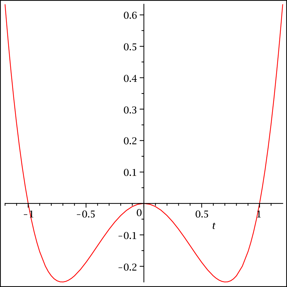
(1) Assume that $n$ is odd. Then the function $w=z^{n}-z^{n-2m}$ has three real points on the real axis, $(-1,0),\,(0,0),\,(1,0)$ and the graph looks like Figure 2. As we see in the Figure, they have one relative maximum $\alpha>0$ and one relative minimum $-\alpha$ . Thus the horizontal line $w=a^{n}$ intersects with this graph at three points if $a^{n}<\alpha$ .

Thus (11) has three real roots for a sufficiently small $a$ . Now we consider the action of $\mathbb{Z}/n\mathbb{Z}$ on $V(\ell_{n,m})$ , we have $3n$ solutions on $V(\ell_{n,m})\cap L(n)$ .

(2) Assume that $n$ is even. In this case, we have to notice that the action of $\mathbb{Z}/n\mathbb{Z}$ on $V(f)\cap L(n)$ is $2:1$ off the origin.

In this case, the graph of $y=t^{n}-t^{n-2m}$ looks like Figure 3.

Thus for a sufficiently small $a>0$ , $t^{n}-t^{n-2m}-a^{n}=0$ has two real roots. Thus by the above remark, it gives $2n/2=n$ roots on $V(\ell_{n,m})\cap L(n)$ . Now we consider the roots on the line $L_{(2j+1)\pi/n}$ , $j=0,\dots,n-1$ . Putting $z=u\zeta,\zeta^{n}=-1$ with $u$ being real, from (10), we get the equality:

(12)

\displaystyle-u^{n}+u^{n-2m}-a^{n}=0.

The graph of $y=-t^{n}+t^{n-2m}$ is the mirror image of Figure 3 with respect to $t$ -axis. Thus $-t^{n}+t^{n-2m}-a^{n}=0$ has 4 real roots. Counting all the roots on the lines in $L(n)^{\prime}$ , it gives 4n/2=2n roots. Thus altogether, we get $3n$ roots. ∎

Now we consider the case $2m\geq n$ .

Lemma 19.

If $2m\geq n>m$ , $\rho(\ell_{n,m})=2n$ for a sufficiently small $a>0$ .

Proof.

(1a) Assume that $2m>n$ and $n$ is odd. The equation of the real solutions of (6 ) reduces to

(13)

\displaystyle z^{2m-n}(z^{n}-a^{n})=1.

It is easy to see that there are two real solutions (one positive and one negative). See Figure 4.

Considering other solutons of the argument $2\pi j/n$ , $j=0,\dots,n-1$ , we get $2n$ solutions.

(1b) Assume that $2m>n$ and $n$ is even. The equation for the real solutions is

z^{2m-n}(z^{n}-a^{n})=1

and it has two real solutions. Thus on the lines $L_{2j\pi/n}$ , $2n/2=n$ solutions. See Figure 5. On the real lines $L_{(2j+1)\pi/n}$ , the equation reduces to

u^{2m-n}(u^{n}+a^{n})=1.

Thus it has $2n/2=n$ solutions on these lines and altogether, we gave $2n$ solutions.

(2) Assume that $n=2m$ . Then (13 ) reduces to

z^{2m}-a^{2m}=1.

This has two real roots on $L_{0}$ and thus we get $2n/2=n$ roots on the lines $L(n)$ . On the lines $\arg\,z=(2j+1)\pi/n$ , putting $z=u\exp(\pi/n)$ , the equation is given by $u^{n}+a^{n}=1$ . This has two roots provided $a<1$ and thus $n$ roots on $L(n)^{\prime}$ . Thus altogether, we get $2n$ roots. ∎

4. Bifurcation of the root and the main result

We considered the extended lens equation for a fixed $a>0$ as in Lemma 18. Note that $z=0$ is a root with multiplicity. We want to change these roots into $2n$ regular roots using a small bifurcation.

(14)

\displaystyle\ell_{n,m}^{\varepsilon}

\displaystyle:=\bar{z}^{m}-\dfrac{z^{n-m}}{z^{n}-a^{n}}+\dfrac{\varepsilon}{z^{m}},\,\,\varepsilon>0.

Note that the mixed polynomial, given by the numerator of $\ell_{n,m}^{\varepsilon}$ (by abuse of the notation, we denote this numerator also by the same notation) satisfies

	$\displaystyle\ell_{n,m}^{\varepsilon}\in L(n_{1}+m;n_{1},m)\subset M(n_{1}+m;n_{1},m)$
	$\displaystyle\text{where}\,\,\qquad n_{1}:=n+m.$

First we observe (14) implies

z^{n}(|z|^{2m}-1+\varepsilon)=\varepsilon a^{n}+|z|^{2m}a^{n}

which implies that $z^{2n}$ is a positive real number as the situation before the bifurcation. We observe that

Proposition 20.

$V(\ell_{n,m}^{\varepsilon})$ is also a subset of $\mathcal{L}(2n)$ and it is $\mathbb{Z}/n\mathbb{Z}$ -invariant.

4.1. The case $m$ is not so big

Assume that $n>2m$ or $n_{1}>3m$ . The following is our main result which generalize the result of Rhie for the case $m=1$ .

Theorem 21.

(1)

Assume that $n>2m$ i.e., $n_{1}>3m$ . For a sufficiently small positive $\varepsilon$ , $\rho(\ell_{n,m}^{\varepsilon})=5(n_{1}-m)$ .
(2)

For the case $n=2m$ , let $f_{2m}$ be as in Corollary 14. Then $f_{2m}\in L(3m;2m,m)$ and $\rho(f_{2m})=5m$ .

Proof.

We prove the assertion for the case $n>2m$ , the assertion for $n=2m$ is in Corollary 14. First observe that $3n$ roots of $\ell_{n,m}$ are all simple. Put them $\xi_{1},\dots,\xi_{3n}$ . Take a small radius $r$ so that the disks $D_{r}(\xi_{j}),\,j=1,\dots,3n$ of radius $r$ centered at $\xi_{j}$ are disjoint each other and they do not contain $0$ and the Jacobian of $\Re\ell_{n,m},\Im\,\ell_{n,m}$ has rank two everywhere on $D_{r}(\xi_{j})$ . Then for any sufficiently small $\varepsilon>$ , there exists a single simple root in $D_{r}(\xi_{j})$ for $\ell_{n,m}^{\varepsilon}=0$ .

First consider the case $n$ being odd. The real root of $\ell_{n,m}^{\varepsilon}=0$ satisfies the equation

(15)		$\displaystyle{\bar{z}}^{m}=\dfrac{z^{n-m}}{z^{n}-a^{n}}+\dfrac{\varepsilon}{z^{m}}\quad\text{or}$
(16)		$\displaystyle f_{\varepsilon}:=\|z\|^{2m}(z^{n}-a^{n})-z^{n}-\varepsilon(z^{n}-a^{n})=0.$

We consider the possible roots which bifurcate from $z=0$ . The second equation (16) is written as

(17)

\displaystyle z^{n}|z|^{2m}-z^{n}(1+\varepsilon)-a^{n}(|z|^{2m}-\varepsilon)=0

$(z^{2m}-\varepsilon)=0$ has two real roots $\alpha_{0+}>0>\alpha_{0-}$ . Take a sufficiently small $s>0$ and consider the disk $B_{0\pm}$ centered at $\alpha_{0\pm}$ of radius $s\varepsilon^{1/2m}$ so that they do not contain zero.

Note that $|z^{2m}-\alpha_{0\pm}|\geq s^{2m}\varepsilon$ on $\partial B_{0\pm}$ . As the other term of $f_{\varepsilon}$ is of order greater than or equal to $\varepsilon^{n/2m}\ll\varepsilon$ . Thus taking $\varepsilon$ small enough, we may assume that $f_{\varepsilon}=0$ has a simple root inside the disk $B_{0+}$ and $B_{0-}$ .

Here is another slightly better argument. We consider the scale change $z=w\varepsilon^{1/2m}$ and put

\begin{split}\tilde{f}_{\varepsilon}(w):=&\frac{1}{\varepsilon}f(w\varepsilon^{1/2m})\\ =&-a^{n}(|w|^{2m}-1)+\varepsilon^{n/2m}w^{n}|w|^{2m}-\varepsilon^{(n-2m)/2m}w^{n}(1+\varepsilon).\end{split}

In this coordinate, $3n$ roots $\xi_{j}$ are far from the origin and we see clearly there are two roots near $w=\pm 1$ as long as $\varepsilon$ is sufficientlt small.

We consider now roots on $L(n)$ . By the $\mathbb{Z}/n\mathbb{Z}$ -invariance, we have also two roots on each $L_{2\pi j/n}$ and thus we get $2n$ simple roots which are bifurcating from $z=0$ . Thus altogether, we get $5n=5(n_{1}-m)$ roots.

We consider now the case $n$ being even. Then every root of (17) on $\arg\,z=2j\pi/n$ are counted twice. Thus we have $n$ roots on these real line. In this case, there are also roots on the real lines $\arg\,z=(2j+1)\pi/n$ . In fact, put $z=u\exp\pi i/n$ in (17). Then the equation in $u$ takes the form:

(18)

\displaystyle-u^{n}|u|^{2m}+u^{n}(1+\varepsilon)-a^{n}(|u|^{2m}-\varepsilon)=0

This has two real roots. Thus we found another $2n/2=n$ roots. Therefore there are $2n$ simple roots which bifurcate from $z=0$ . Thus we have $5n$ roots for $\ell_{n,m}^{\varepsilon}$ in any case. ∎

4.2. Rhie’s equations

Applying Theorem 21, we get lens equation with maximal number of zeros $5(n-1)$ in the form:

\bar{z}=f_{n}(z),\quad f_{n}(z)=\frac{z^{n-2}}{z^{n-1}-a^{n-1}}-\frac{\varepsilon}{z},\,0<\varepsilon\ll a\ll 1

for $n\geq 4$ . For example, for $n=4$ , we can take for example

f_{4}(z)=\frac{z^{2}}{z^{3}-1/5}-\frac{1/800}{z}.

For $n=2,3$ , the previous construction does not work and we need a special care. In fact, we can take $f_{n}$ for $n=2,3$ as follows (Compare with [1]):

f_{2}(z)=\frac{z-1/30}{z^{2}-1/2},\quad f_{3}(z)=\frac{z^{2}-1/1000}{z^{3}-1/8}.

In Figure 7, the red curve is $\Im(numerator(\bar{z}-f_{3}(z))=0$ and the green curve is the zero set of $\Re(numerator(\bar{z}-f_{3}(z))=0$ . The 10 intersections of green and red curves are zeros of $\bar{z}-f_{3}(z)=0$ . Graph is lifted -1 vertically.

4.3. The case $m$ is big

Assume that $2m\geq n>m$ . In this case, we have the following result.

Theorem 22.

Assume that $2m\geq n>m$ . Then for a sufficiently small $\varepsilon>0$ , $\rho(\ell_{n,m}^{\varepsilon})\geq 3n=3(n_{1}-m)$ .

Proof.

We have shown in Lemma 18 that $L_{n,m}$ has $2n$ simple roots. Thus we need to show under the bifurcation equation $\ell_{n,m}^{\varepsilon}$ , we get $n$ further roots.

{\bar{z}}^{m}-\dfrac{z^{n-m}}{z^{n}-a^{n}}-\dfrac{\varepsilon}{z^{m}}=0

is equivalent to

(19)			$\displaystyle\|z\|^{2m}(z^{n}-a^{n})-z^{n}-\varepsilon(z^{n}-a^{n})$	$\displaystyle=0\,\,\text{or}$
(20)			$\displaystyle\|z\|^{2m}(z^{n}-a^{n})-z^{n}(1+\varepsilon)+a^{n}\varepsilon$	$\displaystyle=0$

(I-1) We first consider the case $2m>n$ and $n$ is odd. $-z^{n}(1+\varepsilon)+a^{n}\varepsilon=0$ has one positive root $z=\beta=a\root n \of{\varepsilon/(1+\varepsilon)}$ . By a similar argument as in the previous section, (20) has a simple root near $\beta$ . Thus by the $\mathbb{Z}/n\mathbb{Z}$ -action stability, we have $n$ simple bifurcating roots and altogether, we have $2n+n=3n$ simple roots.

(I-2) Assume that $2m>n$ and $n$ is even. $-z^{n}(1+\varepsilon)+a^{n}\varepsilon=0$ has one positive and one negative roots. Then by the stability (20) has $2n/2=n$ simple roots. To see the roots on $L(n)^{\prime}$ , put $z=u\exp(i\pi/n)$ . Then (20) is reduced to

|u|^{2m}(-u^{n}-a^{n})+u^{n}(1+\varepsilon)+a^{n}\varepsilon=0

We see this has no real root. Thus altogteher, we have $3(n_{1}-m)$ roots.

(II) Assume that $n=2m$ . Then (20) can be written as

(21)

\displaystyle|z|^{2m}z^{2m}-z^{2m}(a^{2m}+1+\varepsilon)+a^{2m}\varepsilon=0

if $z$ real. This has two real roots and adding all roots in the lines of $L(n)$ , we get $2n/2=n$ roots.

Consider other roots on $L(n)^{\prime}$ . Then we can write $z=u\zeta$ with $\zeta^{n}=-1$ and $u\in\mathbb{R}$ and

-|u|^{2m}u^{2m}+u^{2m}(1-a^{2m}+\varepsilon)+a^{2m}\varepsilon=0.

This has no zeros near the origin, as we have assumed $0<a<1$ to have 2n zeros in $L_{n,m}=0$ . Thus the above bifurcation equation has no real root. Thus altogether we conclude $\rho(L_{n,m}^{\varepsilon})=3n=3(n_{1}-m)$ . ∎

4.4. Application

4.4.1. $L^{hs}(n+m;n,m)$

The space of harmonically splitting Lens type polynomials apparently can take bigger number of zeros than generalized lens polynomials. To show this, we start from arbitrary lens equation

\begin{split}\ell_{n}(z):=&\bar{z}-\frac{p(z)}{q(z)},\quad\deg_{z}q=n,\,\deg_{z}p\leq n,\\ \end{split}

Put $k=\rho(\ell_{n})$ . We assume that $0$ is not a root of $\ell_{n}$ for simplicity and $q(z)$ has coefficient 1 for $z^{n}$ . We consider its small purturbation in $L^{hs}(n+m;n,m)$ :

\phi_{t}(z):=-t\bar{z}^{m}+\ell_{n}(z)=-t\bar{z}^{m}+\bar{z}-\frac{p(z)}{q(z)},\,\,1\gg t>0.

We assert

Theorem 23.

For sufficiently small $t>0$ , $\rho(\phi_{t})=k+m-1$ .

Proof.

As before, we identify $\phi_{t},\ell_{n}$ with their numerators. For sufficiently small $t$ and for each zero root $\alpha$ of $\ell_{n}$ , there exists a zero $\alpha^{\prime}$ of $\phi_{t}$ in a neighborhood of $\alpha$ which has the same orientation as $\alpha$ . For $t\neq 0$ , we know that $\beta(\phi_{t})=n-m$ and $\beta(\ell_{n})=n-1$ . Here $\beta(f)$ is the number of zeros of $f$ with sign. See Theorem 2. By the assumption, $\ell_{n}$ has $k$ zeros, say $\alpha_{1},\dots,\alpha_{k}$ and $\beta(\ell_{n})=n-1$ . First we choose a positive number $R$ so that $1/R<|\alpha_{j}|<R$ for $j=1,\dots,5n-5$ . Thus it is clear that $\phi_{t}$ has $k$ zeros near each $\alpha_{j}(\varepsilon)$ with the same sign as $\alpha_{j}$ in the original equation $\ell_{n}=0$ . On the other hand, $\beta(\phi_{t})=n-m,\,t\neq 0$ . Thus $\phi_{\varepsilon}$ has at least $m-1$ new negative zeros.

We assert that $\phi_{t}$ obtains exactly $m-1$ new negative zeros near infinity. To see this near infinity, we change the coordinate $u=1/z$ and consider the numerator: $((-t/\bar{u}^{m}-1/\bar{u})q(1/u)-p(1/u))\,\bar{u}^{m}u^{n}$ . This takes the form

\Phi_{t}=(-t+\bar{u}^{m-1})\,\tilde{q}(u)-\bar{u}^{m}\tilde{p}(u)

where $\tilde{q},\tilde{p}$ are polynomials defined as $\tilde{q}(u)=u^{n}q(1/u),\,\tilde{p}(u)=u^{n}p(1/u)$ . By asumption we can write

\begin{split}\tilde{q}(u)&=1+\sum_{i=1}^{n}b_{i}u^{i}\\ \tilde{p}(u)&=\sum_{i=0}^{n}c_{i}u^{i}.\end{split}

We will prove that for a sufficiently small $t>0$ , there exist exactly $m-1$ zeros $u(t)$ which converges to 0 as $t\to 0$ . The zero set

\{(u,t)\in\mathbb{C}\times\mathbb{R}\,|\,\Phi_{t}(u)=0\}

in $\mathbb{C}\times\mathbb{R}$ is a real algebraic set. Thus we need only check the components which intersect with $t=0$ . We use the Curve selection lemma. Suppose that

(22)		$\displaystyle\Phi_{t(s)}(u(s))$	$\displaystyle\equiv$	$\displaystyle 0,,\,\,t(s)=s^{a},\quad$
(23)		$\displaystyle u(s)$	$\displaystyle=$	$\displaystyle\sum_{j=p}^{\infty}d_{j}s^{j},\,\,d_{p}\neq 0.$

Note that the possible lowest order of $(-t(s)+\bar{u}(s)^{m-1})\tilde{q}(u(s))$ is $\min(a,p(m-1))$ , while the lowest order of the second term $\bar{u}(s)^{m}\tilde{p}(u(s))$ is $pm$ . Thus (22) says

a=p(m-1),\quad-1+{\overline{d}_{p}}^{m-1}=0.

Thus we can write

(24)

\displaystyle d_{p}=\exp(2\pi ji/(m-1)),\quad\exists j,\,0\leq j\leq m-2.

We assert that

Assertion 24.

For a fixed $j$ , there exist a unique $u(s)$ which satisfies (22) and (24).

We prove the coefficients $d_{j}$ of $u(s)$ are uniquely determined by induction. Put

	$\displaystyle(-t(s)+\bar{u}^{m-1}(s)\tilde{q}(u(s))$	$\displaystyle=$	$\displaystyle\sum_{\nu=p(m-1)}^{\infty}\gamma_{\nu}s^{\nu}$
	$\displaystyle\bar{u}(s)^{m}\tilde{p}(u(s))$	$\displaystyle=$	$\displaystyle\sum_{\nu=pm}^{\infty}\delta_{\nu}s^{\nu}.$

We have shown $\gamma_{p(m-1)}=0$ as $d_{p}=\exp(2\pi ji/(m-1))$ . Suppose that $d_{j},\,p\leq j\leq\mu-1$ are uniquely determined. We consider the coefficient of $s^{p(m-2)+\mu}$ in (22). We need to have

\gamma_{p(m-2)+\mu}=\delta_{p(m-2)+\mu}.

Observe that

\gamma_{p(m-2)+\mu}=(m-1)\overline{d}_{p}^{m-1}\overline{d}_{\mu}+r^{\prime}

where $r^{\prime}$ is a polynomial of coefficients $\{\overline{d}_{j},\,j\leq\mu-1\}\cup\{b_{j},\,j=1,\dots,n\}$ . On the other hand, $\delta_{p(m-2)+\mu}$ is a polynomial of coefficients $\{\overline{d}_{j},\,j\leq\mu-1\}\cup\{c_{j},\,j=0,\dots,n\}$ . Thus $d_{\mu}$ is uniquely determined by the equality $\gamma_{p(m-2)+\mu}=\delta_{p(m-2)+\mu}$ . ∎

As $\Phi_{t}\in L^{hs}(n+m;n,m)$ , combining with Theorem 6, we obtain the following.

Corollary 25.

The set of the number of zeros $\rho(f)$ of harmonically splitting lens type polynomials $f\in L^{hs}(n+m;n,m)$ includes $\{n+m-2,n+m,\cdots,5n+m-6\}$ .

4.4.2. The moduli space $M(n+m;n,m)$

Now we consider the bigger class of polynomials $M(n+m;n,m)\supset L^{hs}(n+m;n,m)$ . As $\beta(F)=n-m$ for $F\in M(n+m;n,m)$ , the lowest possible number of zeros of a polynomial in $M(n+m;n,m)$ is $n-m$ . In fact we assert

Corollary 26.

The set $\{\rho(f)\,|\,f\in M(n+m;n,m)\}$ includes $\{n-m,n-m+2,\dots,n+m-2,\dots,5n+m-6\}$ .

Proof.

By Corollary 25, it is enough to show that any of $\{n-m,n-m+2,\dots,n+m-4\}$ can be $\rho$ of some $f\in M(n+m;n,m)$ . Let $j=n-m+2a,\,0\leq a\leq m-2$ . Consider the polynomial

f_{a}(z)=(z^{n-a}\bar{z}^{m-a}-1)(z^{a}-2)(\bar{z}^{a}-3)

Then we see that $\rho(f_{a})=n-m+2a$ and $f_{a}\in M(n+m;n,m)$ . ∎

Example 27.

Consider $M(5;3,2)$ . The possible $\rho$ are $\{1,3,\dots,11\}$ . For $\rho=1,3,5$ , we can take for example mixed polynomials associated with thefollowing polynomials

f(z)=z^{3}\bar{z}^{2}-1,\,(z^{2}\bar{z}-1)(z-2)(\bar{z}-3),\,(z-1)(z^{2}-2)(\bar{z}^{2}-3).

The higher values $\{7,9,11\}$ are given by

\varepsilon\bar{z}^{2}+\bar{z}-\frac{p(z)}{q(z)},\,\deg\,p(z)\leq 3,\,\deg\,q(z)=3,\,\varepsilon\ll 1

where $\bar{z}-\frac{p(z)}{q(z)}=0$ is a lens type equation with $\rho=6,8,10$ .

4.5. Further remark.

4.5.1. $L(n+2m;n+m,m)$ with $2m<n$

We observe that in Theorem 21, $\rho(\ell_{n,m}^{\varepsilon})=5(n_{1}-m)$ with $n_{1}=n+m$ which is exactly the optimal upper bound for $m=1$ . Thus we may expect that the number $5(n_{1}-m)$ might be optimal upper bound for the polynomials in $L(n_{1}+m;n_{1},m)$ . However in the proof for $m=1$ , a result about an attracting or rationally neutral fixed points in complex dynamics played an important role and the the argument there does not apply directly in our case.

4.5.2. $L(2m+m;2m,m)$

Our poynomial $\ell_{2m,m}^{\varepsilon}$ is not good enough. We have seen in Corollary 14 that the mixed polynomial $f_{2m}$ has $5m$ zeros, while our polynomial $\ell_{m,m}^{\varepsilon}$ has only $3m$ zeros.

Problem 28.

•

Determine the upper bound of $\rho$ for $L(n+m;n,m)$ for $n>3m$ .
•

Determine the posssible number of $\rho$ for $L(n+m;n,m)$ . Is it $\{n-m+2k\,|\,0\leq k\leq 2n-2m\}$ ?
•

Determine the upper bound of $\rho$ for $L^{hs}(n+m;n,m)$ or $M(n+m;n,m)$ .
•

Are the subspaces of the moduli $L(n+m;n,m),\,L^{hs}(n+m;n,m),\,M(n+m;n,m)$ with a fixed $\rho$ connected? If not, give an example.

References

[1] P. Bleher, Y. Homma, L. Ji, P. Roeder. Counting zeros of harmonic rational functions and its application to gravitational lensing, Int. Math. Res. Not. IMRN, 8, 2245–2264.
[2] M. Elkadi, A. Galligo. Exploring univariate mixed polynomials of bidegree. Proceeding of SNC’2014, 50–58, 2014.
[3] P. Griffiths and J. Harris. Principles of algebraic geometry. Wiley Classics Library. John Wiley & Sons Inc., New York, 1994. Reprint of the 1978 original.
[4] D. Kahvinson, G. Neumann. On the number of zeros of certain rational harmonic functions, Proc. Amer. Math. Soc. 134, No. 6, 666–675, 2008.
[5] D. Khanvinson, G. Światȩk. On the number of zeros of certain harmonic polynomials. Proc. Amer. Math. Soc. 131 (2003), no. 2, 409–414.
[6] J. Milnor. Lectures on the $h$ -cobordism theorem. Notes by L. Siebenmann and J. Sondow. Princeton University Press, Princeton, N.J., 1965.
[7] M. Oka. Topology of polar weighted homogeneous hypersurfaces. Kodai Math. J., 31(2):163–182, 2008.
[8] M. Oka. On mixed projective curves, Singularities in Geometry and Topology, 133–147, IRMA Lect. Math. Theor. Phys., 20, Eur. Math. Soc., Zürich, 2012.
[9] M. Oka. Intersection theory on mixed curves. Kodai Math. J. 35 (2012), no. 2, 248–267.
[10] M. Oka. Non-degenerate mixed functions. Kodai Math. J., 33(1):1–62, 2010.
[11] V. Blanloeil, M. Oka. Topology of strongly polar weighted homogeneous links. SUT J.Math. 51 ,no. 1(2015), 119–128.
[12] J. Milnor, P. Orlik. Isolated singularities defined by weighted homogeneous polynomials. Topology, 9:385–393, 1970.
[13] A.O. Petters, M.C.Werner Mathematics of Gravitational Lensing: Multiple Imaging and Magnification. General Relativity Gravitation. Vol. 42,9, 2011–2046, 2010.
[14] S.H. Rhie. n-point Gravitational Lenses with $5(n-1)$ Images. arXiv:astro-ph/0305166, May 2003.
[15] J. Seade. On the topology of isolated singularities in analytic spaces, volume 241 of Progress in Mathematics. Birkhäuser Verlag, Basel, 2006.
[16] A.S. Wilmshurst, The valence of harmonic polynomials. Proc. Amer. Math, Soc. 126, 7, 1998, 2077–2081

On the roots of an extended Lens equation and an application

Abstract.

Key words and phrases:

2000 Mathematics Subject Classification

1. Introduction

1.1. Number of roots with sign

Proposition 1.

Theorem 2.

Remark 3.

1.2. Number of roots ignoring the sign

Example 4.

1.3. Lens equation

Proposition 5.

Theorem 6.

Lemma 7.

2. Relation of strongly polar weighted homogeneous polynomials and number of zeros without sign

Proposition 8.

Proof.

Proposition 9.

Proof.

Proposition 10.

Corollary 11.

Remark 12.

Example 13.

3. Extended lens equation

3.0.1. Extended lens equation

3.1. A symmetric case

Corollary 14.

3.2. Generalization of the Rhie’s example

Proposition 15.

Observation 16.

Lemma 17.

3.3. Preliminary result before a bifurcation

Lemma 18.

Proof.

Lemma 19.

Proof.

4. Bifurcation of the root and the main result

Proposition 20.

4.1. The case mm is not so big

Theorem 21.

Proof.

4.2. Rhie’s equations

4.3. The case mm is big

Theorem 22.

Proof.

4.4. Application

4.4.1. Lh​s​(n+m,n,m)L^{hs}(n+m;n,m)

Theorem 23.

Proof.

Assertion 24.

Corollary 25.

4.4.2. The moduli space M⁡(n+m,n,m)M(n+m;n,m)

Corollary 26.

Proof.

Example 27.

4.5. Further remark.

4.5.1. L⁡(n+2​m,n+m,m)L(n+2m;n+m,m) with 2​m<n2m<n

4.5.2. L⁡(2​m+m,2​m,m)L(2m+m;2m,m)

Problem 28.

References

4.1. The case $m$ is not so big

4.3. The case $m$ is big

4.4.1. $L^{hs}(n+m;n,m)$

4.4.2. The moduli space $M(n+m;n,m)$

4.5.1. $L(n+2m;n+m,m)$ with $2m<n$

4.5.2. $L(2m+m;2m,m)$