Galaxy cluster lensing masses in modified lensing potentials

Throughout, we work under the commonly adopted setup for cluster lensing studies (see e.g. Refs. [68, 69, 70] for comprehensive reviews). In particular, we consider a set of source galaxies at redshift $z_{s}$, whose light gets deflected by a galaxy cluster at $z_{d}$. We use $D_{d}$, $D_{s}$ and $D_{ds}$ to denote, respectively, the angular diameter distances between the observer and the lens, the observer and the sources, and the lens and the sources. We assume clusters are spherically symmetric and use the thin-lens approximation in which one neglects the thickness of the galaxy cluster compared to the much larger values of $D_{d}$, $D_{s}$ and $D_{ds}$. We also neglect the lensing distortions induced by foreground and background structures, compared to the lensing signal of the cluster. In our notation, $r=\sqrt{x^{2}+y^{2}}$ is a two-dimensional radial coordinate defined on the lens plane and with origin at the cluster center ($x$ and $y$ are cartesian coordinates); $l$ denotes the optical axis (line-of-sight) direction, perpendicular to the lens plane, and with origin also at the cluster center; and $R=\sqrt{r^{2}+l^{2}}$, is a three-dimensional radial coordinate with origin at the cluster center.

Light rays coming from the sources are deflected at the lens position by an angle $\vec{\alpha}$, which is related to the true (unobserved) angular position, $\vec{\beta}$, and the observed one, $\vec{\theta}$, by

$\displaystyle\vec{\beta}=\vec{\theta}-\vec{\alpha}(\vec{\theta}).$

(1)

The local properties of the lensing signal are fully determined by spatial second derivatives of the scaled projected lensing potential of the galaxy cluster, $\psi$, which is given by

$\displaystyle\psi(\theta=r/D_{d})=\frac{D_{ds}}{D_{d}D_{s}}\frac{2}{c^{2}}\int_{-D_{d}}^{D_{ds}}\Phi_{\rm len}(r,l){\rm d}l,$

(2)

where $c$ is the speed of light and $\Phi_{\rm len}\equiv\left(\Phi+\Psi\right)/2$ is the total three-dimensional lensing potential. The two Newtonian potentials $\Phi$ and $\Psi$ are defined by the perturbed Friedmann-Robertson-Walker (FRW) line element:

$\displaystyle{\rm d}s^{2}=\left(1+2\Psi/c^{2}\right)c^{2}{\rm d}t^{2}-a^{2}\left(1-2\Phi/c^{2}\right){\rm d}{\bf x}^{2},$

(3)

where $a=1/(1+z)$ is the cosmological scale factor ($z$ is the redshift). The Jacobian matrix of the lensing mapping of Eq. (1) is given by

$$\frac{\partial\vec{\beta}}{\partial\vec{\theta}}(\vec{\theta})=\begin{bmatrix}1-\kappa-\gamma_{1}&-\gamma_{2}\\ -\gamma_{2}&1-\kappa+\gamma_{1}\end{bmatrix},$$

(4)

where

	$\displaystyle\kappa(\theta)$	$\displaystyle=$	$\displaystyle\frac{1}{2}\bar{\nabla}^{2}_{\theta}\psi=\frac{1}{2}\left(\partial^{2}_{\theta_{x}}+\partial^{2}_{\theta_{y}}\right)\psi,$		(5)
		$\displaystyle=$	$\displaystyle\frac{D_{d}^{2}}{2}\bar{\nabla}^{2}_{r}\psi=\frac{D_{d}^{2}}{2}\left(\partial^{2}_{x}+\partial^{2}_{y}\right)\psi$

is the lensing convergence¹¹ 1 The overbar on the $\nabla$ operator indicates that it is the two-dimensional Laplacian. Also, note that $r=D_{d}\theta$., and

	$\displaystyle\gamma_{1}$	$\displaystyle=$	$\displaystyle\frac{1}{2}\left(\partial^{2}_{\theta_{x}}-\partial^{2}_{\theta_{y}}\right)\psi,$
	$\displaystyle\gamma_{2}$	$\displaystyle=$	$\displaystyle\partial_{\theta_{x}}\partial_{\theta_{y}}\psi,$		(6)

are the two components of the complex lensing shear, $|\gamma|=\sqrt{\gamma_{1}^{2}+\gamma_{2}^{2}}$. The convergence is responsible for an isotropic focusing (or defocusing) of the light rays, whereas the shear field causes distortions in the shapes of the observed source galaxies.

In lensing studies, one can split the analysis into the weak and strong lensing regimes. In the weak lensing regime, the directly observable quantity is the locally averaged complex ellipticity field in the lens plane, $\left<\epsilon\right>$, which can be constructed from measurements of background galaxy shapes. At each point of the lens field, an average is taken over a number of nearby sources to smooth out the intrinsic ellipticity of the galaxies from that caused by the lens (see e.g. [69, 71, 72]). Observationally, the field $\left<\epsilon\right>$ is directly related to the reduced shear, $g$, (see e.g. Sec. 4 of Ref. [69])

$\displaystyle\left<\epsilon\right>\longleftrightarrow g\equiv\gamma/(1-\kappa).$

(7)

The strong lensing regime takes place in the inner most regions of the lens. There, the lensing quantities $\kappa$ and $\gamma$ become large and the equations become highly nonlinear. As a consequence, highly distorted images like giant arcs or arclets and multiple images of the same background source can form. This happens close to the location of the critical curves of the lens, which are defined as the set of points on the lens plane where the lensing matrix, Eq. (4), becomes singular, i.e.,

$\displaystyle{\rm det}\left(\partial\vec{\beta}/\partial\vec{\theta}\right)=\left(1-\kappa\right)^{2}-\gamma^{2}=0.$

(8)

Observationally, one identifies multiple images and giant-arcs to infer the position and shape of the critical lines. Then, given a theoretical prediction for $\kappa$ and $\gamma$, one can check if ${\rm det}\left(\partial\vec{\beta}/\partial\vec{\theta}\right)$ vanishes at the location of the critical lines.

In GR, in the absence of anisotropic stress, $\Phi=\Psi$, and as a result, the lensing potential is equal to the dynamical potential, $\Phi_{\rm len}=\left(\Phi+\Psi\right)/2=\Phi=\Psi$. Both satisfy the Poisson equation,

$\displaystyle\nabla_{(r,l)}^{2}\Phi{(r,l)}=4\pi G\rho(r,l),$

(9)

where $G$ is Newton’s constant and $\rho(r,l)$ is the three-dimensional density distribution. The lensing convergence is obtained by integrating Eq. (9) along the line of sight,

$\displaystyle\int\nabla^{2}_{(r,l)}\Phi(r,l){\rm d}l=4\pi G\int\rho(r,l){\rm d}l=4\pi G\Sigma(r),$

(10)

where $\Sigma(r)$ is the surface mass density. The left-hand side of this equation can be manipulated as follows:

			$\displaystyle\int\nabla^{2}_{(r,l)}\Phi(r,l){\rm d}l=\int\bar{\nabla}^{2}_{r}\Phi(r,l){\rm d}l+\int\partial^{2}_{l}\Phi(r,l){\rm d}l$		(11)
		$\displaystyle=$	$\displaystyle\bar{\nabla}^{2}_{r}\int\Phi(r,l){\rm d}l+\left[\partial_{l}\Phi(r,l)\right]^{+\infty}_{-D_{d}}\approx\frac{D_{d}D_{s}c^{2}}{2D_{ds}}\bar{\nabla}^{2}_{r}\psi(r)$
		$\displaystyle=$	$\displaystyle\frac{D_{s}c^{2}}{D_{ds}D_{d}}\kappa(r=\theta D_{d}),$

where we have used Eqs. (2) and (5), and also the fact that first spatial derivatives of $\Phi$ are negligible at cosmological distances away from the lens (thin-lens approximation). Combining Eqs. (10) and (11) yields

$\displaystyle\kappa(\theta)=\frac{4\pi G}{c^{2}}\frac{D_{ds}D_{d}}{D_{s}}\Sigma(\theta)\equiv\frac{\Sigma(\theta)}{\Sigma_{c}},$

(12)

where

$\displaystyle\Sigma_{c}=\frac{c^{2}}{4\pi G}\frac{D_{s}}{D_{ds}D_{d}}$

(13)

is called the critical surface mass density for lensing. Therefore, in GR, the calculation of the lensing convergence reduces to the evaluation of the projected two-dimensional density profile of the cluster, which can often be done analytically (see Sec. II.5 below). The Hubble expansion rate in $\Lambda{\rm CDM}$ is given by

$\displaystyle\left(\frac{H(z)}{H_{0}}\right)^{2}=E^{2}(z)$

$\displaystyle=$

$\displaystyle\Omega_{m0}(1+z)^{3}+(1-\Omega_{m0}),$

(14)

where $H_{0}=100h\ {\rm km/s/Mpc}$ is the present-day Hubble expansion rate (the subscript "$0$" denotes present-day values) and $\Omega_{m0}$ is the fractional background energy density of pressureless matter. Here, and throughout, we assume a spatially flat Universe and neglect the contribution to the expansion rate from radiation and massive neutrinos. Equation (14) is used in the calculation of the angular diameter distances that enter Eq. (13) and the relation between radial and angular scales, $r=D_{d}\theta$.

We focus on the cubic sector of the Galileon gravity model [30, 31, 32]. Its action is given by

$\displaystyle S=\int{\rm d}^{4}x\sqrt{-g}\left[\frac{\mathcal{R}}{16\pi G}-\frac{1}{2}c_{2}\mathcal{L}_{2}-\frac{1}{2}c_{3}\mathcal{L}_{3}-\mathcal{L}_{m}\right],$

where $\mathcal{R}$ is the Ricci scalar, $g$ is the determinant of the metric $g_{\mu\nu}$, $c_{2}$ and $c_{3}$ are dimensionless constants, and $\mathcal{L}_{2}$ and $\mathcal{L}_{3}$ are given by

$\displaystyle\mathcal{L}_{2}=\nabla_{\mu}\varphi\nabla^{\mu}\varphi,\ \ \ \ \ \ \ \ \mathcal{L}_{3}=\frac{2}{\mathcal{M}^{3}}\Box\varphi\nabla_{\mu}\varphi\nabla^{\mu}\varphi,$

(16)

in which $\varphi$ is the Galileon field, $\mathcal{M}^{3}=M_{\rm Pl}H_{0}^{2}$, $M_{\rm Pl}^{2}=1/(8\pi G)$ is the reduced Planck mass, $\Box=\nabla^{\mu}\nabla_{\mu}$ is the d’Alembert operator, $\mathcal{L}_{m}$ is the matter Lagrangian density and Greek indices run over $0$, $1$, $2$, $3$. In flat spacetime, the above action is invariant under the Galilean shift $\partial_{\mu}\varphi\rightarrow\partial_{\mu}\varphi+b_{\mu}$ (where $b_{\mu}$ is a constant four-vector). In spherical coordinates, the Poisson equation in the Galileon model leads to the following force law (see Refs. [59, 58] for details about the derivation)

$\displaystyle\frac{\Phi,_{R}}{R}=\frac{GM(<R)}{R^{3}}-\frac{c_{3}}{\mathcal{M}^{3}}\dot{\bar{\varphi}}^{2}\frac{\delta\varphi,_{R}}{R},$

(17)

where $\delta\varphi(R)$ is the spatial perturbation of the Galileon scalar field about the background value, $\bar{\varphi}(z)$, $M(<R)=4\pi\int_{0}^{R}\rho(r^{\prime})r^{\prime 2}{\rm d}r^{\prime}$ is the mass enclosed inside radius $R$ and $,_{R}$ denotes partial differentiation w.r.t. $R$. Equation (17) differs from GR by having an extra source term which is governed by

$\displaystyle\frac{\delta\varphi,_{R}}{R}=\frac{4}{3}\frac{M_{\rm Pl}}{\beta_{2}}\left(\frac{R}{r_{V}}\right)^{3}\left[\sqrt{\left(\frac{r_{V}}{R}\right)^{3}+1}-1\right]\frac{GM(<R)}{R^{3}},$

with

$\displaystyle r_{V}^{3}=\frac{16}{9}\frac{M_{\rm Pl}}{\beta_{1}\beta_{2}\mathcal{M}^{3}}GM(<r),$

(19)

where $\beta_{1}$ and $\beta_{2}$ are two dimensionless functions of time. The quantity $r_{V}$ is a radial scale (often called the Vainshtein radius) that roughly determines the distance from the halo/cluster center within which the modifications to gravity are suppressed. The combination of Eqs. (17), (II.3) and its derivatives leads to

	$\displaystyle\frac{\Phi,_{R}}{R}$	$\displaystyle=$	$\displaystyle\left\{1-\frac{4}{3}\frac{c_{3}}{M_{\rm Pl}\mathcal{M}^{3}}\frac{\dot{\bar{\varphi}}^{2}}{\beta_{2}}\left(\frac{R}{r_{V}}\right)^{3}\left[\sqrt{\left(\frac{r_{V}}{R}\right)^{3}+1}-1\right]\right\}\frac{GM(<R)}{R^{3}},$		(20)
	$\displaystyle\Phi,_{RR}$	$\displaystyle=$	$\displaystyle G\left[\frac{M(<R),_{R}}{R^{2}}-\frac{2M(<R)}{R^{3}}\right]-\frac{3}{4}\frac{c_{3}\beta_{1}\dot{\bar{\varphi}}^{2}}{M_{\rm Pl}^{2}}\left[\sqrt{\left(\frac{r_{V}}{R}\right)^{3}+1}-1+\frac{3}{2}\frac{(r_{V}/R)^{2}}{\sqrt{(r_{V}/R)^{3}+1}}\left(r_{V},_{R}-\frac{r_{V}}{R}\right)\right].$		(21)

In the limit of large $R$, Eq. (20) can be written as (note that $r_{V}^{3}\rightarrow{\rm constant}$ as $R$ increases)

$\displaystyle\frac{\Phi,_{R}}{R}=G_{\rm lin}\frac{M(<R)}{R^{3}},$

(22)

with

$\displaystyle G_{\rm lin}=G\left(1-\frac{2}{3M_{\rm Pl}\mathcal{M}^{3}}\frac{c_{3}\dot{\bar{\varphi}}^{2}}{\beta_{2}}\right),$

(23)

being an effective "linearized" time dependent gravitational strength. On the other hand, when $R$ becomes small, it is straightforward to show that (using, for instance, the NFW expressions shown below)

$\displaystyle\frac{\Phi,_{R}}{R}\approx\frac{GM(<R)}{R^{3}}.$

(24)

That is, at sufficiently small radii, the force in the Galileon model is approximately the same as in GR, which is a direct consequence of the Vainshtein screening mechanism.

In the Cubic Galileon model one also has that $\Phi=\Psi$ [58], which implies, like in GR in the absence of anisotropic stress, that the lensing potential is equal to the dynamical potential. We compute the convergence in the Cubic Galileon model by numerically integrating the three-dimensional Laplacian of the total potential, $\nabla^{2}\Phi$, along the line of sight as

	$\displaystyle\kappa(\theta)$	$\displaystyle=$	$\displaystyle\frac{D_{ds}D_{d}}{D_{s}c^{2}}\int_{-D_{d}}^{\infty}\nabla^{2}_{(r,l)}\Phi(r,l){\rm d}l$
		$\displaystyle=$	$\displaystyle\frac{1}{4\pi G\Sigma_{c}}\int_{-D_{d}}^{\infty}\left(\Phi,_{RR}(r,l)+2\frac{\Phi,_{R}}{R}(r,l)\right){\rm d}l$

(recall that in spherical coordinates, $\nabla^{2}\cdot\rightarrow\cdot,_{RR}+2\frac{\cdot,_{R}}{R}$).

All that is left to specify is the time dependence of the background quantities that enter the above equations of the Galileon model. The time evolution of the Hubble parameter, $\dot{\bar{\varphi}}$, $\beta_{1}$ and $\beta_{2}$ are given, respectively, by [8]

	$\displaystyle E(a)^{2}$	$\displaystyle=$	$\displaystyle\frac{1}{2}\left[\Omega_{m0}a^{-3}+\sqrt{\Omega_{m0}^{2}a^{-6}+4(1-\Omega_{m0})}\right],$		(26)
	$\displaystyle\dot{\bar{\varphi}}$	$\displaystyle=$	$\displaystyle\xi H_{0}/E(a),$		(27)
	$\displaystyle\beta_{1}$	$\displaystyle=$	$\displaystyle\frac{1}{6c_{3}}\left[-c_{2}-\frac{4c_{3}}{\mathcal{M}^{3}}\left(\ddot{\bar{\varphi}}+2H\dot{\bar{\varphi}}\right)+\frac{2c_{3}^{2}}{M_{\rm Pl}^{2}\mathcal{M}^{6}}\dot{\bar{\varphi}}^{4}\right],$		(28)
	$\displaystyle\beta_{2}$	$\displaystyle=$	$\displaystyle\frac{2\mathcal{M}^{3}M_{\rm Pl}}{\dot{\bar{\varphi}}^{2}}\beta_{1}.$		(29)

As in Ref. [8], we take $c_{2}=-1$ and the other two Galileon parameters are determined by $\Omega_{m0}$ as

	$\displaystyle\xi$	$\displaystyle=$	$\displaystyle\sqrt{6(1-\Omega_{m0})},$		(30)
	$\displaystyle c_{3}$	$\displaystyle=$	$\displaystyle 1/(6\xi).$		(31)

We take the model of Refs. [26, 27] as the representative case of a Nonlocal gravity model. The action is given by

$\displaystyle A=\frac{1}{16\pi G}\int{\rm d}x^{4}\sqrt{-g}\left[\mathcal{R}-\frac{m^{2}}{6}\mathcal{R}\Box^{-2}\mathcal{R}-\mathcal{L}_{m}\right].$

(32)

This (nonlocal) action can be cast in a more familiar (local) form given by [73, 74, 75]

	$\displaystyle A$		$\displaystyle=\frac{1}{16\pi G}\int{\rm d}x^{4}\sqrt{-g}\left[\mathcal{R}-\frac{m^{2}}{6}\mathcal{R}S-\xi_{1}\left(\Box U+\mathcal{R}\right)\right.$		(33)
			$\displaystyle\ \ \ \ \ \ \ \ \ \ \ \ \ \ \ \ \ \ \ \ \ \ \ \ \ \ \ \ \ \ \ \ \left.-\xi_{2}\left(\Box S+U\right)-\mathcal{L}_{m}\right],$

where $\xi_{1}$ and $\xi_{2}$ are two Lagrange multipliers and we have introduced two auxiliary scalar fields, $U=-\Box^{-1}\mathcal{R}$ and $S=\Box^{-2}\mathcal{R}$. For completeness, we note that these two formulations are not equivalent and that care must be taken when matching the solutions associated with the above two actions (see e.g. Refs. [75, 76, 77, 25, 78, 79, 80] for a discussion)

Following Refs. [27, 29], for the scales relevant for large scale structure formation, the modifed Poisson equation in this Nonlocal model can be written as

$\displaystyle\nabla^{2}_{(r,l)}\Phi=4\pi G_{\rm eff}(z)\rho(r,l),$

(34)

which takes the same form as in GR, Eq. (9), but with an effective time dependent gravitational strength given by

$\displaystyle G_{\rm lin}=G\left[1-\frac{m^{2}\bar{S}(z)}{3}\right]^{-1},$

(35)

where $\bar{S}$ is the background part of the field $S$. The time evolution of the background quantities in the Nonlocal model has to be obtained by numerically integrating the background differential equations (see e.g. Refs [27, 29]). The parameter $m$ in Eqs. (32) and (33) controls the amount of dark energy in the Universe. In a flat Universe, the value of $m$ is therefore determined by the energy densities of the remaining matter species, which means this Nonlocal gravity model has the same number of free parameters as $\Lambda{\rm CDM}$.

Just as in the cases of $\Lambda{\rm CDM}$ and Cubic Galileon gravity, in the Nonlocal model we also have that $\Phi=\Psi=\Phi_{\rm len}$, in the absence of anisotropic stress. Moreover, since the Poisson equation in this model is obtained from GR by a simple rescaling of the gravitational strength, it follows that the convergence can also be computed analytically as

$\displaystyle\kappa(\theta)=\left(\frac{G_{\rm lin}}{G}\right)\frac{\Sigma(\theta)}{\Sigma_{c}}.$

(36)

Note, however, that the Nonlocal expansion rate must be used in the calculation of the angular diameter distances that enter $\Sigma_{c}$.

Contrary to the case of Galileon gravity, the Nonlocal model does not possess a screening mechanism, which may raise some concerns about the ability of this model to pass Solar System constraints [2]. For instance, Ref. [29] showed that the rate of change of the gravitational strength on cosmological scales, $\dot{G}_{\rm lin}$, if applied directly to Solar System tests, results in the model becoming inconsistent with current lunar laser ranging experiments [81]. However, the time variation of $G_{\rm lin}$ follows from the background expansion rate, and it is not clear what its impact is in the Solar System. In fact, the authors of Refs. [63, 26] have shown that if the cosmological expansion is neglected, i.e. if the spacetime about the Sun is perturbed Minkowskii (as opposed to FRW), then the model predictions become compatible with the current bounds. Here, we shall bear these discussions in mind, but focus instead on the model predictions for cluster scales, which are sufficiently large for one to consider the gravitational strength given by Eq. (35).

In order to compute the lensing convergence in any of the cosmological models considered above, we need to specify the density profile of the lenses, which we model as dark matter haloes with NFW density profiles [64],

$\displaystyle\rho_{\rm NFW}(R,z)=\frac{\rho_{s}(z)}{(R/r_{s})(1+R/r_{s})^{2}}.$

(37)

This profile is fully specified by two parameters known as the scale radius, $r_{s}$, and the characteristic density, $\rho_{s}$. The mass enclosed inside radius $R$ in a NFW halo is given by:

$\displaystyle M_{\rm NFW}(<R)$

$\displaystyle=$

$\displaystyle 4\pi\rho_{s}r_{s}^{3}\left[{\rm ln}\left(1+R/r_{s}\right)-\frac{R/r_{s}}{1+R/r_{s}}\right].$

We define halo masses in the usual way

$\displaystyle M_{\Delta}$

$\displaystyle=$

$\displaystyle\frac{4\pi}{3}\Delta{\rho}_{c}R_{\Delta}^{3},$

(39)

where $R_{\Delta}$ is the radius within which the mean density is equal to $\Delta$ times the critical density of the Universe at a given redshift, $\rho_{c}=3H^{2}(z)/(8\pi G)$. Equating $M_{\Delta}=M_{\rm NFW}(<R_{\Delta})$ one finds

$\displaystyle\rho_{s}=\frac{1}{3}\Delta{\rho}_{c}c_{\Delta}^{3}\left[{\rm ln}\left(1+c_{\Delta}\right)-\frac{c_{\Delta}}{1+c_{\Delta}}\right]^{-1},$

(40)

where we have defined the concentration parameter

$\displaystyle c_{\Delta}=R_{\Delta}/r_{s}.$

(41)

We take $\Delta=200$ (as it is standard in the literature since it is close to the overdensity at virial equilibrium) and instead of characterizing the NFW haloes by $\rho_{s}$ and $r_{s}$, we use the equivalent and more common parametrization in terms of $M_{200}$ and $c_{200}$.

The surface mass density of a NFW halo admits an analytical solution given by [82, 83, 68]

$\displaystyle\Sigma_{\rm NFW}(r=D_{d}\theta)=\int\rho_{\rm NFW}(r,l){\rm d}l=$

(42)

$$=\begin{cases}\frac{2r_{s}\rho_{s}}{x^{2}-1}\left(1-\frac{2}{\sqrt{1-x^{2}}}{\rm arctanh}\left[\sqrt{\frac{1-x}{1+x}}\ \right]\right)&x<1\\ \frac{2r_{s}\rho_{s}}{3}&x=1\\ \frac{2r_{s}\rho_{s}}{x^{2}-1}\left(1-\frac{2}{\sqrt{x^{2}-1}}{\rm arctan}\left[\sqrt{\frac{x-1}{1+x}}\ \right]\right)&x>1\end{cases}$$

where $x=r/r_{s}$. The calculation of the lensing convergence in Galileon gravity also requires the evaluation of the gradient of $M_{\rm NFW}(<R)$, which is given by

$\displaystyle M_{\rm NFW}(<R),_{R}=4\pi\rho_{s}r_{s}^{3}\frac{R}{(r_{s}+R)^{2}}.$

(43)

We use the convergence profile data that was obtained for the CLASH clusters in Ref. [66]. There, the analysis was performed with a numerical algorithm called SaWLens [84], which iteratively reconstructs the lensing potential for each cluster on a two-dimensional grid that covers the cluster field. The analysis is non-parametric, i.e., it makes no assumptions about the mass distribution of the cluster. We refer the reader to Refs. [84, 66, 85] for the details about how SaWLens operates. For the discussion here, what is important to note is that what SawLens actually reconstructs is the lensing potential scaled to a source redshift of infinity, $\psi_{\infty}=\psi(z_{s}=\infty)$, by assuming a fiducial cosmological model. We use $\kappa_{\infty}$ to denote the lensing convergence associated with $\psi_{\infty}$, which is related to the convergence at the true source redshift, $z_{s}$, via

$\displaystyle\kappa_{z_{s}}$

$\displaystyle=$

$\displaystyle Z^{\rm fid}(z_{d},z_{s})\kappa_{\infty},$

(47)

where we use the subscript ${}_{z_{s}}$ to emphasize that $\kappa_{z_{s}}$ corresponds to the convergence associated with $z_{s}$. The function $Z\equiv Z(z_{d},z_{s})$ transports the convergence from a source redshift of infinity to the source redshift that corresponds to the galaxies on each SaWLens grid cell/pixel (we use the words cell and pixel interchangeably). It is given by

$\displaystyle Z^{\rm fid}(z_{d},z_{s})=\frac{D^{\rm fid}_{s,\infty}D^{\rm fid}_{ds}}{D^{\rm fid}_{ds,\infty}D^{\rm fid}_{s}},$

(48)

where the superscript ^fid indicates angular diameter distances that are calculated assuming the fiducial background cosmology and the subscript _∞ means that the calculation assumes that $z_{s}=\infty$. In the reconstruction process of Ref. [66], the fiducial cosmology is a $\Lambda{\rm CDM}$ model with $\Omega_{m0}=0.27$. From hereon, we use $\kappa^{\rm fid}_{\infty}$ to denote the convergence profiles obtained in this way, where the superscript ^fid makes it explicit that the data is linked to the fiducial model. It is therefore important to investigate the extent to which the $\kappa^{\rm fid}_{\infty}$ profiles can be used in studies of alternative cosmologies.

Consider the case that we wish to estimate the lensing masses of the CLASH clusters in a model with a cosmological background that is different from the fiducial model originally used to analyse the observations in Ref. [66]. In principle, we could suitably modify the SaWLens algorithm to reconstruct the convergence maps in the alternative model, $\kappa^{\rm alt}_{\infty}$, instead of $\kappa^{\rm fid}_{\infty}$. However, this would not be practical as it would imply rerunning the entire analysis pipeline for different background cosmologies. A more economical strategy is to note that the two convergence maps, $\kappa^{\rm fid}_{\infty}$ and $\kappa^{\rm alt}_{\infty}$, can be related by

$\displaystyle Z^{\rm fid}(z_{d},z_{s})\kappa^{\rm fid}_{\infty}=Z^{\rm alt}(z_{d},z_{s})\kappa^{\rm alt}_{\infty},$

(49)

where $Z^{\rm alt}$ is defined as in Eq. (48) but with the distances calculated in any alternative, and not the fiducial, cosmology. The above equation holds (up to a correction that we discuss in the next subsection) since both $Z^{\rm fid}\kappa^{\rm fid}_{\infty}$ and $Z^{\rm alt}\kappa^{\rm alt}_{\infty}$ correspond to $\kappa_{z_{s}}$, i.e., the convergence at the true source redshift ²² 2 For example, for $\Lambda{\rm CDM}$ with an alternative background and for fixed surface mass density, for simplicity, Eq. (49) becomes $\Sigma(\theta)/\Sigma_{c}^{\rm alt}=\Sigma(\theta)/\Sigma_{c}^{\rm fid}\longrightarrow\Sigma_{c}^{\rm alt}=\Sigma_{c}^{\rm fid}$.. Using the above equation, the radially binned convergence profiles obtained using the fiducial cosmology in Ref. [66], $\kappa^{\rm fid}_{\infty}(\theta)$, can be directly compared to the prediction of the alternative model $\kappa^{\rm alt}_{\infty}$, provided the latter is multiplied by the factor $Z^{\rm alt}(z_{d},z_{s})/Z^{\rm fid}(z_{d},z_{s})$. This is the approach that we adopt in this paper. Specifically, we aim to obtain constraints on $M_{200}$, $c_{200}$ and $\Omega_{m0}$ in non-fiducial backgrounds by minimizing the $\chi^{2}$ quantity

$\displaystyle\chi^{2}$

$\displaystyle=$

$\displaystyle\overrightarrow{V}\mathcal{C}_{\kappa}^{-1}\overrightarrow{V},$

(50)

where

$\displaystyle\vec{V}_{i}$

$\displaystyle=$

$\displaystyle\kappa^{\rm fid}_{\infty,i}-\Upsilon\kappa_{\infty}^{\rm alt}(M_{200},c_{200},\Omega_{m0},\theta_{i}),$

(51)

is the $i$-th entry of the vector $\vec{V}$; $\kappa^{\rm fid}_{\infty,i}$ is the reconstructed lensing convergence in the $i$-th radial bin, $\theta_{i}$; $\mathcal{C}_{\kappa}$ is the covariance matrix of the radially binned data ³³ 3 The bootstrap realizations used to derive the covariance matrices in Ref. [66] also make use of the fiducial cosmological background. Here, we use the errors as obtained for the fiducial cosmology and do not attempt to estimate the dependence of the covariance matrix on the assumed cosmology. This does not alter our conclusions as this choice only affects the precise size of the confidence intervals, without introducing any important systematics.; and for brevity of notation, we introduce the scaling factor

$\displaystyle\Upsilon(z_{d},z_{s})=\frac{Z^{\rm alt}(z_{d},z_{s})}{Z^{\rm fid}(z_{d},z_{s})}.$

(52)

In Eq. (51), $\kappa_{\infty}^{\rm alt}$ is given by Eq. (12) for $\Lambda{\rm CDM}$, Eq. (II.3) for Galileon gravity and Eq. (36) for Nonlocal gravity, but using $z_{s}=\infty$, in the calculation of $\Sigma_{c}$.

Unless otherwise specified, we assume flat priors on the free parameters, $\Omega_{m0}\in\left[0.1,0.5\right]$, $M_{200}\in\left[0.3,3.0\right]\times 10^{15}M_{\odot}/h$ and $c_{200}\in\left[1,8\right]$.

As discussed above, $\kappa^{\rm fid}_{\infty}$ is reconstructed by applying the transformation of Eq. (47) in each cell of the SaWLens grid that covers the cluster field. In this process, the value of $z_{s}$ is determined by the redshift of the galaxies used to measure the ellipticity field at that pixel, or by the redshift of the galaxies associated with a given multiple image system. On the other hand, our methodology is based on Eq. (49), in which one scales the lensing quantities from $z_{s}=\infty$ to a source redshift $z_{s}$, but neglects the redshift distribution of the background lensed galaxies. The validity of Eq. (49) then becomes linked to the impact of the spread of the redshift distribution of the source galaxies across each cluster field. For the CLASH clusters analysed in Ref. [66], the redshift distribution of the background galaxies is manifest in four main aspects:

(i) in the weak lensing regime, different ellipticity pixels are associated with different source redshifts since the shapes are measured using different galaxies across the cluster field;

(ii) related to the above, the ellipticity of each pixel results from a local average of neighbouring galaxy shapes, which can have different redshifts;

(iii) the ellipticity field used by SaWLens is a combined catalog of measurements from space- and ground-based telescopes, which probe different galaxy redshift ranges. The measurements of these two catalogs (see Ref. [66]) are corrected for this, but assuming the fiducial cosmology;

(iv) in the strong lensing regime, each pixel is associated with the redshift of the multiple images contained within it, which can be different in different multiple image systems for the same cluster and also different from the galaxy populations used in the weak lensing measurements.

To get a feeling for the size of our approximation, we show in Fig. 3 the $z_{s}$ dependence of the factor $\Upsilon$ (Eq. (52)) for the Galileon (red) and Nonlocal (blue) models, and a $\Lambda{\rm CDM}$ model with $\Omega_{m0}=0.4$ (black). The quantity $\Upsilon$ encapsulates all of the dependence on $z_{s}$ in the $\chi^{2}$ minimization used to estimate the cluster parameters. For illustrative purposes, we choose $z_{d}=0.35$. This corresponds roughly to the mean redshift of the CLASH clusters (cf. Table 1), although the exact value is not important for the discussion here. We note that what is relevant is the slope of the curves and not their absolute value. Consider for the sake of argument an extreme case where the source galaxies are distributed between $z_{s}=[1,3]$, but that we choose to use $z_{s}=2$ in Eq. (52). Focusing on the case of the Galileon model, we have that $\Upsilon(z_{s}=1)\approx 1.019$, $\Upsilon(z_{s}=2)\approx 1.011$ and $\Upsilon(z_{s}=3)\approx 1.007$. These values differ by no more than $\approx 1\%$, and hence our choice of $z_{s}$ should not lead to serious biases in the results. The error would be even smaller in the Nonlocal model or $\Lambda{\rm CDM}$ with $\Omega_{m0}=0.40$, since in these cases the $\Upsilon(z_{s})$ curves are shallower than in the Galileon case. The error of neglecting the redshift distribution becomes smaller for higher values of $z_{s}$, for which the curves in Fig. 3 become visibly flatter. This is relevant for strongly lensed systems, which tend to be associated with galaxies at higher redshifts.

In cluster weak lensing studies, it is common to determine an effective source galaxy redshift, $z_{s,\rm eff}$, defined as

$\displaystyle\frac{D_{ds}}{D_{s}}\left(z_{s,\rm eff}\right)=\left<\frac{D_{ds}}{D_{s}}\right>,$

(53)

where $\left<{D_{ds}}/{D_{s}}\right>$ is an average over all source galaxies. Reference [66] quotes $z_{s,\rm eff}$ values for the CLASH clusters (see also Ref. [67]). For example, Abell 209 ($z_{d}=0.206$) has $\left<{D_{ds}}/{D_{s}}\right>=0.75\pm 0.04$ ($1\sigma$), which corresponds to $z_{s,\rm eff}=1.03^{+0.25}_{-0.15}$ (this estimate comes from Table 3 of Ref. [67]). This uncertainty on $z_{s,\rm eff}$ is much smaller than our rather extreme example above ($z_{s}=2\pm 1$), which further convinces us that the approximation of Eq. (49) is a good one. For completeness, we note that the determination of these values of $z_{s,\rm eff}$ involves knowledge of the background cosmology, and hence they are also model dependent. However, again taking Abell 209 as an example, in the Galileon model one has $D_{ds}/D_{s}(z_{s,\rm eff}=1.03)=0.76$, which is well within the uncertainty ($\pm 0.04$) quoted above for this cluster. We can therefore neglect this model dependency and use the values of $z_{s,\rm eff}$ listed in Ref. [66]. In particular, in our $\chi^{2}$ minimization, we shall use the effective source redshift values found for the background sources of the ground-based ellipticity measurements, which we list in Table 1.

To summarize this discussion, although Eq. (49) is only approximate, the results shown in Fig. 3 suggest that our results are insensitive to the exact choice of $z_{s}$.

Before proceeding further into estimating the CLASH cluster masses in modified gravity models, we discuss some other subtle issues that may arise when combining current lensing modelling techniques with modified gravity. Although it turns out these other issues do not play a direct role in the results of this paper, we believe such a discussion is instructive and leads to a clearer and broader understanding of the results of this and other work in the literature.

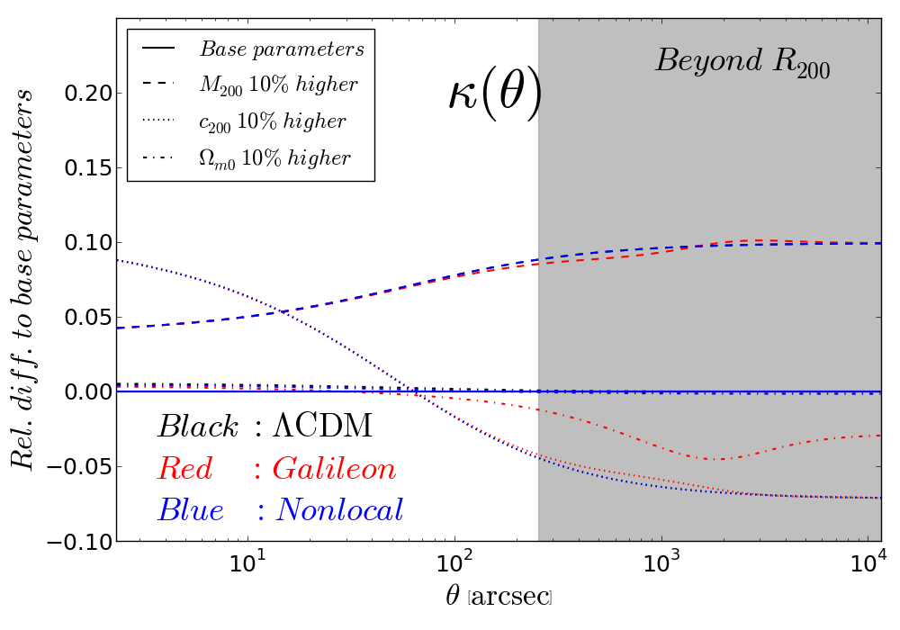
Figure 4 shows the constraints in the $c_{200}$-$M_{200}$ (left), $\Omega_{m0}$-$M_{200}$ (middle) and $\Omega_{m0}$-$c_{200}$ (right) planes for the RX J2129 (blue) and CL J1226 (red) CLASH clusters, assuming a $\Lambda{\rm CDM}$ model. The solid contours show the parameter constraints obtained using a three-dimensional grid search. The gray dots correspond to the points accepted in the chains of a Monte Carlo exploration of the parameter space using the recently developed and publicly-available CosmoSIS⁵⁵ 5 The bitbucket webpage of the CosmoSIS code is https://bitbucket.org/joezuntz/cosmosis/wiki/Home . package [105]. CosmoSIS is a highly modular parameter estimation code, to which we have added likelihood modules based on the convergence profiles of each of the 19 CLASH clusters. Given that our grid code and the MCMC sampler in CosmoSIS are independent ways of sampling the parameter space, it is reassuring that their results agree as shown in Fig. 4. We will be making the CLASH likelihood modules developed in this paper publicly available in future releases of the CosmoSIS standard library.

The middle and right panels of Fig. 4 show that the data from each cluster does not place any meaningful constraints on $\Omega_{m0}$ (this conclusion holds for all of the other CLASH clusters as well). Furthermore, there is no clear degeneracy between $\Omega_{m0}$ and the cluster parameters $M_{200}$, $c_{200}$, which indicates that the constraints on the mass and concentration are unbiased w.r.t. a particular choice of $\Omega_{m0}$. This point is also illustrated by the dashed contours in the left panel of Fig. 4, which show the constraints when the cosmological matter density is held fixed at $\Omega_{m0}=0.27$. The comparison of the solid and dashed contours shows that there is no significant deterioration of the constraints when one allows $\Omega_{m0}$ to be a free parameter. The cases of CL J1226 (red) and MACS J0744 (not shown) are those for which the deterioration is the most pronounced (although still very small). For the rest of the clusters, the two sets of contours (solid and dash) are barely distinguishable, just as in the case of RX J2129 (blue). This illustrates that, in observational determinations of cluster masses from lensing, the impact of assuming a specific value of $\Omega_{m0}$ (as is often done in the literature) is negligible ⁶⁶ 6 The changes in the constraints when one allows $\Omega_{m0}$ to vary are so small that they are of the same magnitude as the error of the approximation of Eq. (49), which is expected to be negligible in any case, as discussed in Sec. IV.2..

To help understand the above result (and others that will follow), it is instructive to look at the impact of $M_{200}$, $c_{200}$ and $\Omega_{m0}$ on the lensing convergence profiles. This is shown in Fig. 5 for $\Lambda{\rm CDM}$ (black), Galileon gravity (red) and Nonlocal gravity (blue). For all models:

• •

  an increase in $c_{200}$ (keeping all other parameters fixed) tilts the convergence profile, boosting its amplitude in the inner regions and lowering it in the outer regions of the halo;

• •

  larger mass values enhance the lensing convergence on all scales shown, with the effect being slightly more pronounced at large radii⁷⁷ 7 Note that for $\theta\gtrsim 10^{2}{\rm arcsec}$, the effects of increasing halo mass start to become degenerate with the effects of decreasing the concentration. Strong lensing analysis, which probes the inner most regions of the cluster, therefore helps to break this concentration-mass degeneracy. Reference [67] also determines the lensing profiles of some of the CLASH clusters used in Ref. [66]. However, the latter includes strong-lensing constraints in the analysis, which allows for more accurate concentration estimations. This is why we choose to work with the results of Ref. [66].;

• •

  A boost in $\Omega_{m0}$ has three main effects. First, it increases the value of $\rho_{c}(z)$ at the cluster redshift, which effectively increases the density of the halo for fixed $M_{200}$ (recall the discussion of Sec. III). This should boost the convergence at small radii. Second, an increase in $\Omega_{m0}$ also has an impact on the cosmological distances that enter $\Sigma_{c}$, which has the overall effect of lowering the amplitude of $\kappa$, by a constant factor. Third, a change in $\Omega_{m0}$ also changes the angular diameter distance to the cluster, $D_{d}$, which causes horizontal shifts in the lensing convergence, when plotted as a function of the observed angular scales $\theta=D_{d}/r$.

The net effect of varying $\Omega_{m0}$ results in almost no visible shift (dot-dashed) in the amplitude of $\kappa$ for the radial scales that are better probed by the CLASH radially binned profiles, $\theta\lesssim 500-700\ {\rm arcsec}$ (cf. Fig. 7). This is why the constraints on $\Omega_{m0}$ in Fig. 4 are so weak. We note also that since the effect of $\Omega_{m0}$ is always subdominant w.r.t. the effects of varying $M_{200}$ and $c_{200}$ (in terms of fractional change), it is unlikely that future lensing data from experiments such as EUCLID [106] and LSST [107] will change this conclusion.

From hereonin, we fix the cosmological matter density to be $\Omega_{m0}=0.27$ for all our models. In this way, the $\Lambda{\rm CDM}$ model becomes the fiducial one used in Ref. [66]. This value is also consistent with the CMB observational constraints for the Cubic Galileon and Nonlocal models as found, respectively, by Ref. [8] and Ref. [28].

Figure 6 shows the constraints on the $c_{200}$-$M_{200}$ plane obtained for each of the CLASH clusters in $\Lambda{\rm CDM}$ (black), Galileon (red) and Nonlocal gravity (blue) cosmologies. The dots indicate the position of the best-fitting values. The best-fitting lensing convergence profiles are shown in Fig. 7 (what is shown is $\Upsilon\kappa_{\infty}(\theta)$). The concentration-mass relation of the CLASH clusters for the three models is shown in Fig. 8, together with results from N-body simulations [108, 61, 29]. First, we note that our cluster mass and concentration estimates for $\Lambda{\rm CDM}$ are in agreement with those obtained in Ref. [66]. Second, these three figures all show that the constraints on the cluster parameters are, within errorbars, the same in the three cosmological models. Although there are tiny differences in the resulting best-fitting values of $M_{200}$ and $c_{200}$ for the three models ($\lesssim 5\%$), they all lie well within the $1\sigma$ limits (whose precision varies within $\sim 50\%-80\%$). The shapes of the contours are also remarkably similar and the goodness-of-fit is essentially the same in all models, as can be seen by comparing the respective $\chi^{2}$ values in Fig. 6. In Fig. 7, one notes that for almost all of the clusters, the best-fitting convergence profiles underpredict the data points at large angular scales (although well within the errorbars). However, close to the edge of the clusters, the contribution from the surrounding large scale structure may have a non-negligible impact. This can partly explain why the data points tend to go up at large scales, as investigated, for instance, in Ref. [109].

The shaded bands in Fig. 8 show the best-fitting mean concentration-mass relations found in N-body simulations for the $\Lambda{\rm CDM}$ (gray) model in Ref. [108] ⁸⁸ 8 See Fig. 9 of Ref. [66] for the comparison of the CLASH $c_{200}$-$M_{200}$ relation in $\Lambda{\rm CDM}$ with other relations in the literature., the Cubic Galileon model (red) in Ref. [61] and the Nonlocal model (blue) in Ref. [29]. In these bands, the lower and upper bounds correspond, respectively, to the relations at $z=0.666$ ($a=0.60$) and $z=0$ ($a=1$) (this redshift range is approximately that of the CLASH clusters). Figure 8 shows that there is good agreement between the simulation results and the concentration/mass estimates of the CLASH clusters in the three models of gravity. However, there are a number of issues that prevent a direct comparison between the simulation results and the estimated concentration and mass values. First, the shaded bands of the Galileon and Nonlocal models in Fig. 8 have been extrapolated to masses larger than the mass range used to fit the best-fitting concentration-mass relations in the simulations of Refs. [61] and [29]. Second, the concentration-mass relation was fitted using all haloes, without applying any selection criteria to consider only relaxed ones [110]. This may be particularly relevant for the CLASH clusters, which are characterized by regular X-ray surface brightness morphologies [65], and are therefore expected to be relaxed and close to virial equilibrium (see also Refs. [111, 112] for a recent discussion on the impact of baryonic processes in the density profiles of clusters). Third, the concentration-mass relation in the simulations was obtained by fitting NFW profiles to the three-dimensional spherically averaged mass distribution of the haloes, whereas the symbols in Fig. 8 are the values obtained by also assuming spherical symmetry, but fitting to two-dimensional (projected) lensing convergence profiles (see e.g. Sec.6.2 of Ref. [66] for an analysis of the impact of this projection bias in the CLASH sample). Finally, the upper and lower bounds of the bands correspond to the mean relation found in the simulations, but the intrinsic scatter around the mean concentration-mass relation should also be taken into account. Nevertheless, to guide the eye, we opted to keep the simulation results in Fig. 8, but advise that further work is needed before performing a more thorough comparison (see the analysis of Ref. [113] in $\Lambda$CDM models for an illustration of the steps to follow).

The left panel of Fig. 9 shows the best-fitting lensing convergence for all of the CLASH clusters in the Galileon (red) and Nonlocal (blue) cosmologies, plotted as the respective difference to the best-fitting profiles in $\Lambda{\rm CDM}$. As expected from the above results, on the scales that are probed by the CLASH data, $\theta\lesssim 500-700\ {\rm arcsec}$, the three models are in very good agreement. In the case of the Galileon model, this is because the screening is very effective on these scales inside $R_{200}$ (Ref. [114] finds a similar screening efficiency inside $R_{200}$ for DGP gravity, which employs also the Vainshtein mechanism). This can be noted by comparing the enhancement in the amplitude of $\kappa$ on larger scales, where the screening becomes less efficient. In the case of the Nonlocal model, although the modifications to the gravitational strength are not screened, they are not strong enough to have a significant impact on the lensing convergence profiles. We therefore conclude that, for the case of the CLASH clusters analysed here, the impact of modifying the lensing gravitational potential according to Cubic Galileon or Nonlocal gravity is completely negligible in the estimation of their lensing masses.

Before this paper, there have been other works investigating the impact of Galileon-like effects on cluster lensing profiles. Reference [103] used a parametrization of the fifth force, which was constrained using the stacked cluster lensing shear profiles from Refs. [97, 98]. Their parametrization encompasses the Galileon model studied here, and for this case, there is good agreement with our conclusions. Reference [102] performed similar investigations, but took as a test case a model inspired by massive gravity. The authors do not consider the time evolution of the cosmological background and their equations of motion include higher order terms than the Galileon model studied here, which prevents a direct comparison with our results. A particularly interesting feature described in Ref. [102] is that some model parameters predict a "dip" in the amplitude of the convergence profiles, which happens for $r\lesssim R_{200}$ (see e.g. Fig. 4 of Ref. [102]). These scales are sufficiently well probed by the lensing data, which allows some of these specific models to be ruled out already. Such features, however, do not show up in our convergence profiles for the Cubic Galileon model (cf. Fig. 7), but which is a different model from the one studied in Ref. [102]. In the context of $f(R)$ models, although the lensing signal is not modified directly, it can be via modified mass distributions. For instance, the enhanced dynamical potential in these models boosts the accretion rate of matter onto the clusters, which results in an excess of mass in their infall region. This can be probed with lensing measurements, as was done in Ref. [115]. Since the Galileon and Nonlocal models also directly modify the dynamical potential, then in principle, similar investigations can be performed. In the case of these models, the lensing signal should be amplified both by the excess of mass that surrounds the cluster, and by the intrinsically enhanced lensing effects. A detailed investigation of this is, however, beyond the scope of the present paper.

References

- [1] P. Ade et al. (Planck Collaboration)(2015), arXiv:1502.01589 [astro-ph.CO]
- [2] C. M. Will, Living Rev.Rel. 17, 4 (2014), arXiv:1403.7377 [gr-qc]
- [3] T. Clifton, P. G. Ferreira, A. Padilla, and C. Skordis, PHYSREP 513, 1 (Mar. 2012), arXiv:1106.2476 [astro-ph.CO]
- [4] A. Joyce, B. Jain, J. Khoury, and M. Trodden(2014), arXiv:1407.0059 [astro-ph.CO]
- [5] B. Jain and P. Zhang, Phys.Rev. D78, 063503 (2008), arXiv:0709.2375 [astro-ph]
- [6] D. Huterer, D. Kirkby, R. Bean, A. Connolly, K. Dawson, et al., Astropart.Phys. 63, 23 (2015), arXiv:1309.5385 [astro-ph.CO]
- [7] B. Jain, A. Joyce, R. Thompson, A. Upadhye, J. Battat, et al.(2013), arXiv:1309.5389 [astro-ph.CO]
- [8] A. Barreira, B. Li, C. Baugh, and S. Pascoli, JCAP 1408, 059 (2014), arXiv:1406.0485 [astro-ph.CO]
- [9] K. Koyama(2015), arXiv:1504.04623 [astro-ph.CO]
- [10] T. P. Sotiriou and V. Faraoni, Rev.Mod.Phys. 82, 451 (2010), arXiv:0805.1726 [gr-qc]
- [11] G. Dvali, G. Gabadadze, and M. Porrati, Phys.Lett. B485, 208 (2000), arXiv:hep-th/0005016 [hep-th]
- [12] P. Zhang, M. Liguori, R. Bean, and S. Dodelson, Phys.Rev.Lett. 99, 141302 (2007), arXiv:0704.1932 [astro-ph]
- [13] F. Schmidt, PRD 81, 103002 (May 2010), arXiv:1003.0409 [astro-ph.CO]
- [14] J. Schwab, A. S. Bolton, and S. A. Rappaport, APJ 708, 750 (Jan. 2010), arXiv:0907.4992 [astro-ph.CO]
- [15] T. L. Smith, ArXiv e-prints(Jul. 2009), arXiv:0907.4829 [astro-ph.CO]
- [16] T. Y. Lam, T. Nishimichi, F. Schmidt, and M. Takada, Physical Review Letters 109, 051301 (Aug. 2012), arXiv:1202.4501 [astro-ph.CO]
- [17] T. Y. Lam, F. Schmidt, T. Nishimichi, and M. Takada, Phys.Rev. D88, 023012 (2013), arXiv:1305.5548 [astro-ph.CO]
- [18] Y. Zu, D. Weinberg, E. Jennings, B. Li, and M. Wyman, Mon.Not.Roy.Astron.Soc. 445, 1885 (2014), arXiv:1310.6768 [astro-ph.CO]
- [19] H. Wilcox, D. Bacon, R. C. Nichol, P. J. Rooney, A. Terukina, et al.(2015), arXiv:1504.03937 [astro-ph.CO]
- [20] A. Terukina and K. Yamamoto, Phys.Rev. D86, 103503 (2012), arXiv:1203.6163 [astro-ph.CO]
- [21] F. Schmidt, A. Vikhlinin, and W. Hu, PRD 80, 083505 (Oct. 2009), arXiv:0908.2457 [astro-ph.CO]
- [22] L. Lombriser, A. Slosar, U. Seljak, and W. Hu, PRD 85, 124038 (Jun. 2012), arXiv:1003.3009 [astro-ph.CO]
- [23] M. Cataneo, D. Rapetti, F. Schmidt, A. B. Mantz, S. W. Allen, et al.(2014), arXiv:1412.0133 [astro-ph.CO]
- [24] S. Deser and R. Woodard, Phys.Rev.Lett. 99, 111301 (2007), arXiv:0706.2151 [astro-ph]
- [25] S. Deser and R. Woodard, JCAP 1311, 036 (2013), arXiv:1307.6639 [astro-ph.CO]
- [26] M. Maggiore and M. Mancarella, Phys.Rev. D90, 023005 (2014), arXiv:1402.0448 [hep-th]
- [27] Y. Dirian, S. Foffa, N. Khosravi, M. Kunz, and M. Maggiore, JCAP 1406, 033 (2014), arXiv:1403.6068 [astro-ph.CO]
- [28] Y. Dirian, S. Foffa, M. Kunz, M. Maggiore, and V. Pettorino(2014), arXiv:1411.7692 [astro-ph.CO]
- [29] A. Barreira, B. Li, W. A. Hellwing, C. M. Baugh, and S. Pascoli, JCAP 1409, 031 (2014), arXiv:1408.1084 [astro-ph.CO]
- [30] A. Nicolis, R. Rattazzi, and E. Trincherini, Phys. Rev. D 79, 064036 (2009)
- [31] C. Deffayet, G. Esposito-Farèse, and A. Vikman, Phys. Rev. D 79, 084003 (2009)
- [32] C. Deffayet, S. Deser, and G. Esposito-Farese, Phys.Rev. D80, 064015 (2009), arXiv:0906.1967 [gr-qc]
- [33] G. Gabadadze, Phys.Lett. B681, 89 (2009), arXiv:0908.1112 [hep-th]
- [34] C. de Rham, Phys.Lett. B688, 137 (2010), arXiv:0910.5474 [hep-th]
- [35] C. de Rham, G. Gabadadze, and A. J. Tolley, Phys.Rev.Lett. 106, 231101 (2011), arXiv:1011.1232 [hep-th]
- [36] C. de Rham and G. Gabadadze, Phys.Lett. B693, 334 (2010), arXiv:1006.4367 [hep-th]
- [37] C. de Rham and G. Gabadadze, Phys.Rev. D82, 044020 (2010), arXiv:1007.0443 [hep-th]
- [38] C. de Rham, G. Gabadadze, L. Heisenberg, and D. Pirtskhalava, Phys.Rev. D83, 103516 (2011), arXiv:1010.1780 [hep-th]
- [39] S. Hassan and R. A. Rosen, JHEP 1202, 126 (2012), arXiv:1109.3515 [hep-th]
- [40] P. Brax and P. Valageas, Phys.Rev. D90, 023507 (2014), arXiv:1403.5420 [astro-ph.CO]
- [41] P. Brax and P. Valageas, Phys.Rev. D90, 023508 (2014), arXiv:1403.5424 [astro-ph.CO]
- [42] A. Barreira, P. Brax, S. Clesse, B. Li, and P. Valageas(2014), arXiv:1411.5965 [astro-ph.CO]
- [43] E. Babichev, C. Deffayet, and R. Ziour, Int.J.Mod.Phys. D18, 2147 (2009), arXiv:0905.2943 [hep-th]
- [44] G. W. Horndeski, Int.J.Theor.Phys. 10, 363 (1974)
- [45] M. Wyman, Physical Review Letters 106, 201102 (May 2011), arXiv:1101.1295 [astro-ph.CO]
- [46] Y. Park and M. Wyman(2014), arXiv:1408.4773 [astro-ph.CO]
- [47] R. Mandelbaum, A. Slosar, T. Baldauf, U. Seljak, C. M. Hirata, R. Nakajima, R. Reyes, and R. E. Smith, MNRAS 432, 1544 (Jun. 2013), arXiv:1207.1120 [astro-ph.CO]
- [48] R. A. Battye, A. Moss, and J. A. Pearson(2014), arXiv:1409.4650 [astro-ph.CO]
- [49] C. D. Leonard, T. Baker, and P. G. Ferreira(2015), arXiv:1501.03509 [astro-ph.CO]
- [50] G.-B. Zhao, L. Pogosian, A. Silvestri, and J. Zylberberg, Phys.Rev. D79, 083513 (2009), arXiv:0809.3791 [astro-ph]
- [51] A. Barreira, B. Li, C. M. Baugh, and S. Pascoli, PRD 86, 124016 (Dec. 2012), arXiv:1208.0600 [astro-ph.CO]
- [52] J. Enander, Y. Akrami, E. Mortsell, M. Renneby, and A. R. Solomon(2015), arXiv:1501.02140 [astro-ph.CO]
- [53] R. Kimura, T. Kobayashi, and K. Yamamoto, PRD 85, 123503 (Jun. 2012), arXiv:1110.3598 [astro-ph.CO]
- [54] A. Vainshtein, Phys. Lett. B 39, 393 (1972), ISSN 0370-2693
- [55] K. Koyama, G. Niz, and G. Tasinato, Phys.Rev. D88, 021502 (2013), arXiv:1305.0279 [hep-th]
- [56] E. Babichev and C. Deffayet, Class.Quant.Grav. 30, 184001 (2013), arXiv:1304.7240 [gr-qc]
- [57] A. Barreira, B. Li, C. Baugh, and S. Pascoli, Phys.Rev. D90, 023528 (2014), arXiv:1404.1365 [astro-ph.CO]
- [58] A. Barreira, B. Li, C. M. Baugh, and S. Pascoli, JCAP 1311, 056 (2013), arXiv:1308.3699 [astro-ph.CO]
- [59] A. Barreira, B. Li, W. A. Hellwing, C. M. Baugh, and S. Pascoli, JCAP 1310, 027 (2013), arXiv:1306.3219 [astro-ph.CO]
- [60] B. Li, A. Barreira, C. M. Baugh, W. A. Hellwing, K. Koyama, et al., JCAP 1311, 012 (2013), arXiv:1308.3491 [astro-ph.CO]
- [61] A. Barreira, B. Li, W. A. Hellwing, L. Lombriser, C. M. Baugh, et al., JCAP 1404, 029 (2014), arXiv:1401.1497 [astro-ph.CO]
- [62] P. Ade et al. (Planck Collaboration)(2015), arXiv:1502.01595 [astro-ph.CO]
- [63] A. Kehagias and M. Maggiore, JHEP 1408, 029 (2014), arXiv:1401.8289 [hep-th]
- [64] J. F. Navarro, C. S. Frenk, and S. D. White, Astrophys.J. 490, 493 (1997), arXiv:astro-ph/9611107 [astro-ph]
- [65] M. Postman and et al, APJS 199, 25 (Apr. 2012), arXiv:1106.3328 [astro-ph.CO]
- [66] J. Merten, M. Meneghetti, M. Postman, K. Umetsu, A. Zitrin, et al.(2014), arXiv:1404.1376 [astro-ph.CO]
- [67] K. Umetsu, E. Medezinski, M. Nonino, J. Merten, M. Postman, et al., Astrophys.J. 795, 163 (2014), arXiv:1404.1375 [astro-ph.CO]
- [68] K. Umetsu, ArXiv e-prints(Feb. 2010), arXiv:1002.3952 [astro-ph.CO]
- [69] M. Bartelmann and P. Schneider, Phys.Rept. 340, 291 (2001), arXiv:astro-ph/9912508 [astro-ph]
- [70] M. Bartelmann, Classical and Quantum Gravity 27, 233001 (Dec. 2010), arXiv:1010.3829 [astro-ph.CO]
- [71] T. D. Kitching, J. Rhodes, C. Heymans, R. Massey, Q. Liu, M. Cobzarenco, B. L. Cragin, A. Hassaine, D. Kirkby, E. J. Lok, D. Margala, J. Moser, M. O’Leary, A. M. Pires, and S. Yurgenson, ArXiv e-prints(Apr. 2012), arXiv:1204.4096 [astro-ph.CO]
- [72] R. Massey, H. Hoekstra, T. Kitching, J. Rhodes, M. Cropper, J. Amiaux, D. Harvey, Y. Mellier, M. Meneghetti, L. Miller, S. Paulin-Henriksson, S. Pires, R. Scaramella, and T. Schrabback, MNRAS 429, 661 (Feb. 2013), arXiv:1210.7690 [astro-ph.CO]
- [73] S. Nojiri and S. D. Odintsov, Phys.Lett. B659, 821 (2008), arXiv:0708.0924 [hep-th]
- [74] S. Capozziello, E. Elizalde, S. Nojiri, and S. D. Odintsov, Phys.Lett. B671, 193 (2009), arXiv:0809.1535 [hep-th]
- [75] N. Koshelev, Grav.Cosmol. 15, 220 (2009), arXiv:0809.4927 [gr-qc]
- [76] T. S. Koivisto, AIP Conf.Proc. 1206, 79 (2010), arXiv:0910.4097 [gr-qc]
- [77] A. O. Barvinsky, Phys.Rev. D85, 104018 (2012), arXiv:1112.4340 [hep-th]
- [78] M. Maggiore, Phys.Rev. D89, 043008 (2014), arXiv:1307.3898 [hep-th]
- [79] S. Foffa, M. Maggiore, and E. Mitsou, Phys.Lett. B733, 76 (2014), arXiv:1311.3421 [hep-th]
- [80] S. Foffa, M. Maggiore, and E. Mitsou, Int.J.Mod.Phys. A, to appear(2014), arXiv:1311.3435 [hep-th]
- [81] J. G. Williams, S. G. Turyshev, and D. H. Boggs, Phys.Rev.Lett. 93, 261101 (2004), arXiv:gr-qc/0411113 [gr-qc]
- [82] M. Bartelmann, Astron.Astrophys. 313, 697 (1996), arXiv:astro-ph/9602053 [astro-ph]
- [83] C. Oaxaca Wright and T. G. Brainerd, ArXiv Astrophysics e-prints(Aug. 1999), astro-ph/9908213
- [84] J. Merten, M. Cacciato, M. Meneghetti, C. Mignone, and M. Bartelmann, Astron.Astrophys. 500, 681 (2009), arXiv:0806.1967 [astro-ph]
- [85] J. Merten, D. Coe, R. Dupke, R. Massey, A. Zitrin, E. S. Cypriano, N. Okabe, B. Frye, F. G. Braglia, Y. Jiménez-Teja, N. Benítez, T. Broadhurst, J. Rhodes, M. Meneghetti, L. A. Moustakas, L. Sodré, Jr., J. Krick, and J. N. Bregman, MNRAS 417, 333 (Oct. 2011), arXiv:1103.2772 [astro-ph.CO]
- [86] J. Kneib, R. Ellis, I. Smail, W. Couch, and R. Sharples, Astrophys.J. 471, 643 (1996), arXiv:astro-ph/9511015 [astro-ph]
- [87] T. J. Broadhurst et al. (ACS Collaboration), Astrophys.J. 621, 53 (2005), arXiv:astro-ph/0409132 [astro-ph]
- [88] G. P. Smith, J.-P. Kneib, I. Smail, P. Mazzotta, H. Ebeling, et al., Mon.Not.Roy.Astron.Soc. 359, 417 (2005), arXiv:astro-ph/0403588 [astro-ph]
- [89] A. Halkola, S. Seitz, and M. Pannella, Mon.Not.Roy.Astron.Soc. 372, 1425 (2006), arXiv:astro-ph/0605470 [astro-ph]
- [90] E. Jullo, J.-P. Kneib, M. Limousin, A. Eliasdottir, P. Marshall, et al., New J.Phys. 9, 447 (2007), arXiv:0706.0048 [astro-ph]
- [91] A. Zitrin, T. Broadhurst, K. Umetsu, D. Coe, N. Benítez, B. Ascaso, L. Bradley, H. Ford, J. Jee, E. Medezinski, Y. Rephaeli, and W. Zheng, MNRAS 396, 1985 (Jul. 2009), arXiv:0902.3971 [astro-ph.CO]
- [92] M. Oguri, PASJ 62, 1017 (Aug. 2010), arXiv:1005.3103 [astro-ph.CO]
- [93] A. B. Newman, T. Treu, R. S. Ellis, D. J. Sand, C. Nipoti, J. Richard, and E. Jullo, APJ 765, 24 (Mar. 2013), arXiv:1209.1391 [astro-ph.CO]
- [94] E. Jullo, S. Pires, M. Jauzac, and J.-P. Kneib, Mon.Not.Roy.Astron.Soc. 437, 3969 (2014), arXiv:1309.5718 [astro-ph.CO]
- [95] T. L. Johnson, K. Sharon, M. B. Bayliss, M. D. Gladders, D. Coe, et al., Astrophys.J. 797, 48 (2014), arXiv:1405.0222 [astro-ph.CO]
- [96] A. Monna, S. Seitz, N. Greisel, T. Eichner, N. Drory, et al., Mon.Not.Roy.Astron.Soc. 438, 1417 (2014), arXiv:1308.6280 [astro-ph.CO]
- [97] K. Umetsu, T. Broadhurst, A. Zitrin, E. Medezinski, D. Coe, and M. Postman, APJ 738, 41 (Sep. 2011), arXiv:1105.0444 [astro-ph.CO]
- [98] M. Oguri, M. B. Bayliss, H. Dahle, K. Sharon, M. D. Gladders, P. Natarajan, J. F. Hennawi, and B. P. Koester, MNRAS 420, 3213 (Mar. 2012), arXiv:1109.2594 [astro-ph.CO]
- [99] M. Jauzac, B. Clément, M. Limousin, J. Richard, E. Jullo, et al., Mon.Not.Roy.Astron.Soc. 443, 1549 (2014), arXiv:1405.3582 [astro-ph.CO]
- [100] M. Jauzac, E. Jullo, D. Eckert, H. Ebeling, J. Richard, et al., Mon.Not.Roy.Astron.Soc. 446, 4132 (2015), arXiv:1406.3011 [astro-ph.CO]
- [101] M. Jauzac, J. Richard, E. Jullo, B. Clément, M. Limousin, et al.(2014), arXiv:1409.8663 [astro-ph.CO]
- [102] T. Narikawa, T. Kobayashi, D. Yamauchi, and R. Saito, Phys.Rev. D87, 124006 (2013), arXiv:1302.2311 [astro-ph.CO]
- [103] T. Narikawa and K. Yamamoto, JCAP 5, 016 (May 2012), arXiv:1201.4037 [astro-ph.CO]
- [104] K. Umetsu, T. Broadhurst, A. Zitrin, E. Medezinski, and L.-Y. Hsu, APJ 729, 127 (Mar. 2011), arXiv:1011.3044 [astro-ph.CO]
- [105] J. Zuntz, M. Paterno, E. Jennings, D. Rudd, A. Manzotti, et al.(2014), arXiv:1409.3409 [astro-ph.CO]
- [106] R. Laureijs, J. Amiaux, S. Arduini, J. . Auguères, J. Brinchmann, R. Cole, M. Cropper, C. Dabin, L. Duvet, A. Ealet, and et al., ArXiv e-prints(Oct. 2011), arXiv:1110.3193 [astro-ph.CO]
- [107] LSST Dark Energy Science Collaboration, ArXiv e-prints(Nov. 2012), arXiv:1211.0310 [astro-ph.CO]
- [108] A. R. Duffy, J. Schaye, S. T. Kay, and C. Dalla Vecchia, Mon.Not.Roy.Astron.Soc. 390, L64 (2008), arXiv:0804.2486 [astro-ph]
- [109] M. Oguri and T. Hamana, MNRAS 414, 1851 (Jul. 2011), arXiv:1101.0650 [astro-ph.CO]
- [110] A. F. Neto, L. Gao, P. Bett, S. Cole, J. F. Navarro, et al., Mon.Not.Roy.Astron.Soc. 381, 1450 (2007), arXiv:0706.2919 [astro-ph]
- [111] M. Schaller, C. S. Frenk, R. G. Bower, T. Theuns, A. Jenkins, et al.(2014), arXiv:1409.8617 [astro-ph.CO]
- [112] M. Schaller, C. S. Frenk, R. G. Bower, T. Theuns, J. Trayford, et al.(2014), arXiv:1409.8297 [astro-ph.CO]
- [113] M. Meneghetti, E. Rasia, J. Vega, J. Merten, M. Postman, et al., Astrophys.J. 797, 34 (2014), arXiv:1404.1384 [astro-ph.CO]
- [114] B. Falck, K. Koyama, and G.-b. Zhao(2015), arXiv:1503.06673 [astro-ph.CO]
- [115] L. Lombriser, F. Schmidt, T. Baldauf, R. Mandelbaum, U. Seljak, and R. E. Smith, PRD 85, 102001 (May 2012), arXiv:1111.2020 [astro-ph.CO]
- [116] W. A. Hellwing, A. Barreira, C. S. Frenk, B. Li, and S. Cole, Phys.Rev.Lett. 112, 221102 (2014), arXiv:1401.0706 [astro-ph.CO]
- [117] G.-B. Zhao, B. Li, and K. Koyama, Physical Review Letters 107, 071303 (Aug. 2011), arXiv:1105.0922 [astro-ph.CO]
- [118] A. P. Hearin(2015), arXiv:1501.02798 [astro-ph.CO]
- [119] C. Heymans, L. Van Waerbeke, L. Miller, T. Erben, H. Hildebrandt, H. Hoekstra, T. D. Kitching, Y. Mellier, P. Simon, C. Bonnett, J. Coupon, L. Fu, J. Harnois Déraps, M. J. Hudson, M. Kilbinger, K. Kuijken, B. Rowe, T. Schrabback, E. Semboloni, E. van Uitert, S. Vafaei, and M. Velander, MNRAS 427, 146 (Nov. 2012), arXiv:1210.0032 [astro-ph.CO]
- [120] P. Ade et al. (XXX Collaboration)(2015), arXiv:1502.01590 [astro-ph.CO]
- [121] P. Melchior, P. Sutter, E. S. Sheldon, E. Krause, and B. D. Wandelt, Mon.Not.Roy.Astron.Soc., 2922(2014), arXiv:1309.2045 [astro-ph.CO]
- [122] J. Clampitt and B. Jain(2014), arXiv:1404.1834 [astro-ph.CO]
- [123] E. Krause, T.-C. Chang, O. Doré, and K. Umetsu, APJL 762, L20 (Jan. 2013), arXiv:1210.2446 [astro-ph.CO]
- [124] Y.-C. Cai, N. Padilla, and B. Li(2014), arXiv:1410.1510 [astro-ph.CO]
- [125] A. Barreira, B. Li, and M. Cautun, et al; in preparation