Asymptotics and statistical inferences on independent and non-identically distributed bivariate Gaussian triangular arrays

Let $\{(X_{ni},Y_{ni}),1\leq i\leq n,n\geq 1\}$ be independent bivariate Gaussian triangular arrays, and let $\rho_{ni}$ denote the correlation coefficient of $(X_{ni},Y_{ni})$, $1\leq i\leq n$. The bivariate maxima $\operatorname*{\mathbf{M}}_{n}$ are defined componentwise by

$${\operatorname*{\mathbf{M}}}_{n}=(M_{n1},M_{n2})=\left(\max_{1\leq i\leq n}X_{ni},\max_{1\leq i\leq n}Y_{ni}\right).$$

For the asymptotic distribution of $\operatorname*{\mathbf{M}}_{n}$, Sibuya (1960) showed that $M_{n1}$ and $M_{n2}$ are asymptotic independent if $\rho_{ni}=\rho\in(-1,1)$, which coincides with the tail asymptotic independence of Gaussian copula, see Embrechts et al. (2002). For the case of $\rho_{ni}=\rho_{n}$, Hüsler and Reiss (1989) derived that

$\displaystyle\lim_{n\to\infty}\sup_{x\in\operatorname*{\mathbb{R}},y\in\operatorname*{\mathbb{R}}}\left|\operatorname*{\mathbb{P}}\left({M}_{n1}\leq b_{n}+\frac{x}{b_{n}},{M}_{n2}\leq b_{n}+\frac{y}{b_{n}}\right)-H_{\lambda}(x,y)\right|=0$

(1.1)

provided that the following Hüsler-Reiss condition

$$\lim_{n\to\infty}b_{n}^{2}(1-\rho_{n})=2\lambda^{2}$$

(1.2)

holds with $\lambda\in[0,\infty]$ ( the converse assertion is proved by Kabluchko et al. (2009)), where the norming constant $b_{n}$ satisfies

$$1-\Phi(b_{n})=\frac{1}{n},$$

(1.3)

where $H_{\lambda}(x,y)$, the so-called Hüsler-Reiss max-stable distribution, is given by

$$H_{\lambda}(x,y)=\exp\left(-\Phi\left(\lambda+\frac{x-y}{2\lambda}\right)e^{-y}-\Phi\left(\lambda+\frac{y-x}{2\lambda}\right)e^{-x}\right)$$

with $\Phi(x)$ standing for the standard Gaussian distribution. Obviously, components of $\operatorname*{\mathbf{M}}_{n}$ are asymptotic dependent when $\lambda<\infty$.

For Hüsler-Reiss model, the asymptotic behavior of the dynamic copula version of normalized $\operatorname*{\mathbf{M}}_{n}$ has also been studied in recent literature. Under the Hüsler-Reiss condition (1.2), Frick and Reiss (2013) considered the asymptotic behaviors of the distribution of $(n(\max_{1\leq i\leq n}\Phi(X_{ni})-1),n(\max_{1\leq i\leq n}\Phi(Y_{ni})-1))$. Allowing $\rho_{ni}$ to depend on both $i$ and $n$, Liao et al. (2014a) extended the result in Frick and Reiss (2013) by assuming that

$$\rho_{ni}=1-m(i/n)/\log n$$

(1.4)

for some positive function $m(x)$. For other work related to Hüsler-Reiss model and its extensions, see, e.g., Hashorva (2005, 2006), Hashorva et al. (2012), Hashorva and Weng (2013), Kabluchko (2011), Engelke et al. (2014), Das et al. (2014) and reference therein.

The objective of this paper is to derive the first and the second-order distributional expansions of the dynamic Hüsler-Reiss model with $\rho_{ni}$ given by (1.4) and establish statistical inferences related to the function $m(x)$. For the convergence rates and higher-order expansions of univariate extremes, we refer to de Haan and Resnick (1996), Nair (1981), Liao et al. (2014b) and reference therein. For the convergence rates of bivariate extremes, see de Haan and Peng (1997) for the general case. For the special case of the bivariate Hüsler-Reiss model, Hashorva et al. (2014) established the higher-order distributional expansions of $\operatorname*{\mathbf{M}}_{n}$, and Liao and Peng (2014) established the uniform convergence rate of (1.1). Liao and Peng (2015) also derived the second-order expansion of the joint distribution of normalized maximum and minimum. So far, there are no studies on the convergence and distributional expansion of $\operatorname*{\mathbf{M}}_{n}$ under the assumption that $(X_{ni},Y_{ni})^{\prime}s$ are not identically distributed. The main goal of this paper is to fill this gap. Borrowing the ideas from Liao et al. (2014a), we derive in this paper the limit distribution of the normalized maxima $\operatorname*{\mathbf{M}}_{n}$ if the function $m(i/n)$ in (1.4) satisfies some regular conditions, and establish its second-order distributional expansion provided that the convergence rate of $\max_{1\leq i\leq n}m(i/n)$ is given. Furthermore, parametric estimation of $m(x)$ is considered through maximum likelihood estimation. The asymptotic properties of the estimators can be employed to test the condition proposed by Hüsler and Reiss (1989).

The rest of this paper is organized as follows. In section 2, we provide the main results and statistical procedures. A simulation study and some real data analysis are presented in Section 3. All proofs are given in Section 4.

In this section we examine the finite sample performance of the proposed estimators by drawing independent $(X_{n1},Y_{n1}),\cdots,(X_{nn},Y_{nn})$ with $(X_{ni},Y_{ni})$ following the bivariate Gaussian distribution with coefficient $\rho_{ni}=1-m(i/n)/\log n$. We consider $n=1000,3000$ or $10000$, and repeat $1000$ times.

First we consider $m(s)=\alpha$ with $\alpha=1$ or $10$, and calculate the average and mean squared error for $\hat{\alpha}$. We can observe from Table 1 that i) the averages of $\hat{\alpha}$ is near by the true value $\alpha$; ii) small mean squared errors show the robustness of $\hat{\alpha}$. Next the case of $m(s)=\alpha+\beta s$ is considered. Table 2 reports the averages and mean squared errors for estimator $(\hat{\alpha},\hat{\beta})$. As $n$ becomes large, the accuracy of all estimators improve. Finally, we consider the case of $m(s)=\alpha+\beta s^{\gamma}$ with sample size $n=10000$. The simulation shows that all estimators are closer to their true values with small mean squared errors, cf. Table 3 for details.

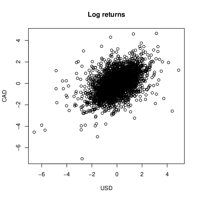
For the applications, we consider four couples of real data sets: The first is the log-returns of the exchange rates between US dollar and British pound and those between Canadian dollar and British pound from April 3, 2000 to November 11, 2014. The second is the log-returns of the Shanghai Stock Exchange composite index (SSE Composite) and ShenZhen Stock Exchange Composite index (SZSE Composite) from March 4, 1996 to November 12, 2014. The third is the log-returns of the CSI 300 index and CSI 300 index futures from April 16, 2010 to November 13, 2014. The forth is the wave and surge heights in southwest England which comprise 2894 wave heights and 2894 surge heights. All time series are plotted in Figure 1.

First, we calculate the $i$th sample correlation for each couple of the mentioned data sets by using $\{(X_{n1},Y_{n1}),\cdots,(X_{ni},Y_{ni})\}$. Figures 2-5 show respectively that each tends to constant ultimately. Now we estimate the correlation $\rho=1-m(i/n)/\log(n)$ by assuming that $m(s)$ is a constant, which also are illustrated by Figures 2-5, respectively. The constancy of $m(s)$ shows that observations are identically distributed.

The aim of this section is to prove our main results. In the sequel, let $F_{i}(x,y)$ denote the distribution function of $(X_{ni},Y_{ni})$, $1\leq i\leq n$; and let $u_{n}(x)=b_{n}+x/b_{n}$ for notational simplicity.

It follows from (1.3) that

$$b_{n}=(2\log n)^{\frac{1}{2}}-\frac{\log\log n+\log 4\pi}{2({2}\log n)^{\frac{1}{2}}}+o\left(\frac{1}{(\log n)^{\frac{1}{2}}}\right),$$

(4.1)

which implies that $b_{n}^{2}\sim 2\log n$ as $n\to\infty$. Combining with (1.4), we have

			$\displaystyle\frac{u_{n}(x)-\rho_{ni}u_{n}(z)}{\sqrt{1-\rho_{ni}^{2}}}$		(4.2)
		$\displaystyle=$	$\displaystyle\sqrt{\frac{1-\rho_{ni}}{1+\rho_{ni}}}b_{n}+\frac{x-z}{b_{n}\sqrt{1-\rho_{ni}^{2}}}+\sqrt{\frac{1-\rho_{ni}}{1+\rho_{ni}}}\frac{z}{b_{n}}$
		$\displaystyle=$	$\displaystyle\sqrt{\frac{m(\frac{i}{n})}{(\log n)\left(2-\frac{m(\frac{i}{n})}{\log n}\right)}}(2\log n)^{\frac{1}{2}}\left(1-\frac{\log\log n+\log 4\pi}{4\log n}+o\left(\frac{1}{\log n}\right)\right)$
			$\displaystyle+\frac{x-z}{(2\log n)^{\frac{1}{2}}\left(1-\frac{\log\log n+\log 4\pi}{4\log n}+o\left(\frac{1}{\log n}\right)\right)\sqrt{\frac{m(\frac{i}{n})}{(\log n)}\left(2-\frac{m(\frac{i}{n})}{\log n}\right)}}$
			$\displaystyle+\sqrt{\frac{m(\frac{i}{n})}{(\log n)\left(2-\frac{m(\frac{i}{n})}{\log n}\right)}}\frac{z}{(2\log n)^{\frac{1}{2}}\left(1-\frac{\log\log n+\log 4\pi}{4\log n}+o\left(\frac{1}{\log n}\right)\right)}$
		$\displaystyle=$	$\displaystyle\sqrt{m\left(\frac{i}{n}\right)}+\frac{x-z}{2\sqrt{m\left(\frac{i}{n}\right)}}-\frac{\log\log n}{4\log n}\sqrt{m\left(\frac{i}{n}\right)}+\frac{\log\log n}{8\log n}\frac{x-z}{\sqrt{m\left(\frac{i}{n}\right)}}+O\left(\frac{1}{\log n}\right)+O\left(\frac{z}{\log n}\right)$

for large $n$.

By using the inequality $\left|\Phi(x)-\Phi(y)\right|\leq|x-y|$ for any $x,y\in\operatorname*{\mathbb{R}}$, we have

$\displaystyle\left|\Phi\left(\frac{u_{n}(x)-\rho_{ni}u_{n}(z)}{\sqrt{1-\rho_{ni}^{2}}}\right)-\Phi\left(\sqrt{m\left(\frac{i}{n}\right)+\frac{x-z}{2\sqrt{m\left(\frac{i}{n}\right)}}}\right)\right|\leq(1+|z|)O\left(\frac{\log\log n}{\log n}\right)+(1+|z|)O\left(\frac{1}{\log n}\right)$

for large $n$ and any $z\in\operatorname*{\mathbb{R}}$, which implies that

			$\displaystyle\frac{1}{n}\sum_{i=1}^{n}\int_{y}^{\infty}\Phi\left(\frac{u_{n}(x)-\rho_{ni}u_{n}(z)}{\sqrt{1-\rho_{ni}^{2}}}\right)\exp\left(-z-\frac{z^{2}}{2b_{n}^{2}}\right)dz$		(4.3)
		$\displaystyle=$	$\displaystyle\frac{1}{n}\sum_{i=1}^{n}\int_{y}^{\infty}\Phi\left(\sqrt{m\left(\frac{i}{n}\right)}+\frac{x-z}{2\sqrt{m\left(\frac{i}{n}\right)}}\right)e^{-z}dz(1+o(1))$
		$\displaystyle\to$	$\displaystyle\int_{0}^{1}\int_{y}^{\infty}\Phi\left(\sqrt{m(t)}+\frac{x-z}{2\sqrt{m(t)}}\right){e^{-z}}dzdt$
		$\displaystyle=$	$\displaystyle-e^{-x}+e^{-y}\int_{0}^{1}\Phi\left(\sqrt{m(t)}+\frac{x-y}{2\sqrt{m(t)}}\right)dt+e^{-x}\int_{0}^{1}\Phi\left(\sqrt{m(t)}+\frac{y-x}{2\sqrt{m(t)}}\right)dt$

as $n\to\infty$.

Note that by Castro (1987) and (1.3),

$\displaystyle n^{-1}=1-\Phi(b_{n})=\frac{\varphi(b_{n})}{b_{n}}\left(1-b_{n}^{-2}+O(b_{n}^{-4})¡¡\right)$

(4.4)

for large $n$, and Nair (1981) showed that

$\displaystyle\lim_{n\to\infty}b_{n}^{2}\left(-n(1-\Phi(u_{n}(x)))+e^{-x}\right)=\frac{x^{2}+2x}{2}e^{-x}.$

(4.5)

Combining with (4.3), we have

			$\displaystyle-\sum_{i=1}^{n}\left(1-F_{i}(u_{n}(x),u_{n}(y))\right)$		(4.6)
		$\displaystyle=$	$\displaystyle-n\left(1-\Phi(u_{n}(x))\right)-n^{-1}\left(1+b_{n}^{-2}+O(b_{n}^{-4})\right)\sum_{i=1}^{n}\int_{y}^{\infty}\Phi\left(\frac{u_{n}(x)-\rho_{ni}u_{n}(s)}{\sqrt{1-\rho_{ni}^{2}}}\right){\exp\left(-s-\frac{s^{2}}{2b_{n}^{2}}\right)}ds$
		$\displaystyle\to$	$\displaystyle-e^{-x}-\int_{0}^{1}\int_{y}^{\infty}\Phi\left(\sqrt{m(t)}+\frac{x-s}{2\sqrt{m(t)}}\right)e^{-s}dsdt$
		$\displaystyle=$	$\displaystyle-e^{-y}\int_{0}^{1}\Phi\left(\sqrt{m(t)}+\frac{x-y}{2\sqrt{m(t)}}\right)dt-e^{-x}\int_{0}^{1}\Phi\left(\sqrt{m(t)}+\frac{y-x}{2\sqrt{m(t)}}\right)dt$

as $n\to\infty$, which implies the desired result.

The proof is complete. ∎

By Taylor expansion with Lagrange reminder term, we have

			$\displaystyle\Phi\left(\frac{u_{n}(x)-\rho_{ni}u_{n}(z)}{\sqrt{1-\rho_{ni}^{2}}}\right)$
		$\displaystyle=$	$\displaystyle\Phi\left(\sqrt{m\left(\frac{i}{n}\right)}+\frac{x-z}{2\sqrt{m\left(\frac{i}{n}\right)}}\right)+\varphi\left(\sqrt{m\left(\frac{i}{n}\right)}+\frac{x-z}{2\sqrt{m\left(\frac{i}{n}\right)}}\right)\left(\frac{u_{n}(x)-\rho_{ni}u_{n}(z)}{2\sqrt{m\left(\frac{i}{n}\right)}}-\sqrt{m\left(\frac{i}{n}\right)}-\frac{x-z}{2\sqrt{m\left(\frac{i}{n}\right)}}\right)$
			$\displaystyle+\frac{1}{2}\theta\varphi(\theta)\left(\frac{u_{n}(x)-\rho_{ni}u_{n}(z)}{\sqrt{1-\rho_{ni}^{2}}}-\sqrt{m\left(\frac{i}{n}\right)}-\frac{x-z}{2\sqrt{m\left(\frac{i}{n}\right)}}\right)^{2},$

where

$$\min\left(\frac{u_{n}(x)-\rho_{ni}u_{n}(z)}{\sqrt{1-\rho_{ni}^{2}}},\sqrt{m\left(\frac{i}{n}\right)}+\frac{x-z}{2\sqrt{m\left(\frac{i}{n}\right)}}\right)<\theta<\max\left(\frac{u_{n}(x)-\rho_{ni}u_{n}(z)}{\sqrt{1-\rho_{ni}^{2}}},\sqrt{m\left(\frac{i}{n}\right)}+\frac{x-z}{2\sqrt{m\left(\frac{i}{n}\right)}}\right).$$