Actors vs Shared Memory: two models at work
on Big Data application frameworks

Silvia Crafa Affiliation: Università di Padova, Italy Luca Tronchin Affiliation: Università di Padova, Italy

Abstract

This work aims at analyzing how two different concurrency models, namely the shared memory model and the actor model, can influence the development of applications that manage huge masses of data, distinctive of Big Data applications. The paper compares the two models by analyzing a couple of concrete projects based on the MapReduce and Bulk Synchronous Parallel algorithmic schemes. Both projects are doubly implemented on two concrete platforms: Akka Cluster and Managed X10. The result is both a conceptual comparison of models in the Big Data Analytics scenario, and an experimental analysis based on concrete executions on a cluster platform.

1 Introduction

In recent years the concept of Big Data has attracted the general interest since valuable information can be extracted from the analysis of large volumes of data. Even if there is not a reference size, Big Data generally refers to those data sets whose size requires hardware and software tools beyond the common machines capabilities. A crucial aspect of Big Data computing is concurrency, since data must be processed in parallel by distributing the computation across multiple machines. To facilitate this process, specific application frameworks are becoming widespread as they autonomously manage the parallelism and distribution of the operations, requiring the user to only define the processing of small amounts of data. In this work we focus on a couple of algorithmic schemes that lie under the major Big Data application frameworks, that is MapReduce and the Bulk Synchronous Parallel model. MapReduce is a model inspired by map and reduce functions from the functional programming, through which many real world tasks can be expressed (e.g., sorting and searching tasks [4, 7, 9]). The Bulk Synchronous Parallel (BSP) model has recently gained great interest because of its ability to process graphs of enormous size, such as social or location graphs, by deeply exploiting the work distribution on several machines ([10, 1, 15]). These two algorithmic schemes are abstract enough to be implemented on any platform; there are indeed several implementations based on the most popular languages. We just mention here the major frameworks: Google’s MapReduce [5], Apache Hadoop and Apache Spark for MapReduce, and Google’s Pregel [11] and Apache Giraph for BSP.

This work aims at studying how specific implementations of MapReduce and BSP take advantage of the platform on which they are implemented. In particular, we address the crucial core of the programming paradigm, that is the concurrency model that shapes the platform design. We then focus on the actor model and the shared memory model, in order to assess how they affect the development of Big Data applications and their performance.

To concretely instantiate the shared memory model, we consider the X10 platform, which is specifically designed for scale-out distributed programming with a partitioned global address space. As for the actor model, we consider the Scala language and the Akka Cluster library. Both platforms allow the development of applications that run on the Java Virtual Machine (JVM), which thus provides a common basis to compare the applications and to bring out the differences that specifically depend on each model. Even if established Big Data application frameworks are available both for X10 and Scala technologies (e.g., [13] and [16]), we implement from scratch the MapReduce and BSP frameworks in a lightweight but effective way, so to better value and compare the distinctive features of the two underlying programming models.

For the same reason it is also necessary to identify some tractable problem whose significance can be appreciated ( $i$ ) at the abstract level, when comparing concurrency models, ( $ii$ ) at the structural level, when comparing the programming styles, and ( $iii$ ) at the experimental level, when comparing performances. We then apply the MapReduce scheme to the sorting of a one-dimensional distributed array spanning over a set of nodes, and we instantiate BSP on the exploration of a distributed sparse graph. Both problems are implemented twice: as an X10 application and as an Akka application. In the MapReduce projects we focus on remote parallelism, that is we let each node just host sequential computation, while in the BSP projects we study both local and remote parallelization opportunities.

Both the code style comparison and the experimental results attest that X10 excels with inter-node parallelism, distinctive of MapReduce, while Akka shines on intra-node concurrency better scaling to the higher local concurrency degree required by BSP.

Structure of the paper

In Section 2 we overview the main characteristics of the two platforms under examination. In Section 3 we illustrate the MapReduce and BSP algorithmic schemes together with their instantiation on the problems of sorting a distributed array and exploring a sparse graph. In Section 4 we report on the implementation of the two problems both in X10 and Akka, going into a comparison of the resulting code styles and drawing some insight about the impact of the different concurrency models. In Section 5 we provide the details of the experimental comparison and we put forward our assessment of the impact of the two concurrency models in the Big Data Analytics scenario. Finally, we draw our conclusions in Section 6 pointing to future research directions.

2 The programming platforms

X10[6, 2] is an open-source object-oriented programming language designed for productive high performance programming of parallel and multi-core computer systems. It is designed around a partitioned global address space (PGAS): the computation is spread over a set of places, each of which holds data and hosts asynchronous activities that operate on local data. Objects residing in one place may contain references (GlobalRefs) to objects residing in other places. However, X10 enforces a strong locality property: an object’s mutable state cannot be accessed through a remote reference to that object. Therefore the language provides the at(p)S construct that permits the current activity to change its place of execution to p, execute S at place p and return, leaving behind activities that may have been spawned during the execution of S. The values of variables used in S but defined outside S are serialized, transmitted to p, and de-serialized to reconstruct a binding environment in which S is executed.

Activities represent lightweight threads in X10 and can be created and started locally with the async S statement. Dually, the finish S statement executes S and waits for the termination of every activity spawned by S either locally or at a remote place. Given the underlying shared-memory model, atomic execution is provided by the atomic S construct, which guarantees that a single local activity at a time can enter its atomic block. Finally, X10 supports global data-structures spanning multiple places. For instance, as described in Section 4, we will take advantage of the DistArray object, which represents a global reference to a distributed array and provides useful methods that simplify the centralized control of its distributed elements.

As far as Akka is concerned, in this work we draw on the combination of the Scala language and Akka’s actor implementation included in its standard library. Actors are objects that encapsulate state and behavior; they communicate exclusively by asynchronously exchanging messages which are placed into the recipient’s mailbox. The environment takes care of the actor mailbox and guarantees that a single messages is processed at a time, hence as long as only the actor has access to its local variables, the absence of race conditions is enforced by the model. As for distribution, we rely on the Akka Remote and Akka Cluster libraries, which support referential transparency in remote actors communications, that is the developer can use the actor references (ActorRef) to send messages without having to worry about whether the recipient resides on the same node of the sender or not. There are two main types of actor references: local actor references and remote actor references. The remote references contain the information necessary to identify the actors on different nodes. The actor references may be exchanged between actors through messages or can be calculated since an actor can be identified in the system by combining the node address with the actor path in the node. Finally, we mention that in order to monitor and manage the cluster status, Akka Cluster relies on the gossip protocol to support the elastic and resilient nature of the system. This component exchanges a bunch of implicit messages that are not directly controlled by the user, which however only cause a small overhead in actor communications.

3 Two BigData algorithmic schemes

3.1 MapReduce

In the MapReduce algorithmic scheme, a distributed computation is specified as a (possibly repeated) sequence of Map, Shuffle and Reduce steps, parametrized around a pair of functions supplied by the user. The first function, mapper, processes a (key,value) pair to generate an intermediate (key,value) pair, and the second function, reducer, merges all the values associated with the same intermediate key to output a final (key,value) pair. More precisely, the algorithm corresponds to the following sequence of steps, depicted in Figure 1:

•

Initialization step: data are loaded in the initial (key,value) pairs, in order to process them in the Map step.
•

Map step: each node applies the mapper function to the local (key,value) pairs obtaining intermediate pairs.
•

Shuffle step: each node redistributes intermediate pairs produced by the mapper function, such that all values belonging to one key are located on the same node.
•

Reduce step: each node now processes each group of pairs, per key, in parallel, using the reducer function.
•

Sink step: it processes the Reduce output to apply some final operation like storing the results.

Figure 1: Diagram of MapReduce.

As for the distribution, each node performs the Init step independently, in parallel to the others. Subsequently each node performs the Map step on data produced by the local Init step (dashed line boxes). In the same way, data processed by a Reduce step are then processed by a Sink step on the same node (dotted line boxes). As for the Shuffle step, the user defines a partition function to determine the target node depending on the output key of the Map step.

Figure 1 shows that in each node the Map and Reduce steps can be locally parallelized by applying the mapper and reducer functions to different portions of local data. Indeed, MapReduce can take advantage of locality of data, by processing them on or near the storage assets in order to reduce the distance over which they must be transmitted. Therefore, at every step, the nodes only work on their own data portion, eliminating data races, and local computation proceeds independently of the remote one. Hence the change in the number of nodes does not involve the computation, but only affects performance.

While this process can often appear inefficient compared to algorithms that are more sequential, or designed to run on a single machine, MapReduce can be applied to significantly larger data-sets than “commodity” servers can handle (a large server farm can use MapReduce to sort a petabyte of data in only a few hours[4]). However, when designing a MapReduce algorithm, the author needs to choose a good trade-off[14] between the computation costs and the communication costs of the shuffle step. In particular, the partition function and the amount of data transferred after the Map step can have a large impact on the performance; indeed, in the Big Data scenario communication cost often dominates the computation cost.

3.2 Sorting a distributed array with MapReduce

We now apply the MapReduce algorithmic scheme to the sorting of a one-dimensional distributed array spanning over a set of nodes. We assume that the cluster has a fixed number of $N_{\mathit{nodes}}$ nodes, that are ordered from $0$ to $N_{\mathit{nodes}}-1$ . We let the value of the input array to be randomly generated and we let the array to be equally distributed over the nodes so that the indexes of the array slice allocated on any node $p$ are greater than the indexes of the slice allocated on the node $p-1$ , as depicted in Figure 2. We also require the output array to be sorted, to be equally distributed over the nodes, and the elements at node $p$ must be greater than those at node $p-1$ , for any $p\in 1,...,N_{\mathit{nodes}}-1$ .

Refer to caption — Figure 2: An array spanning multiple nodes.

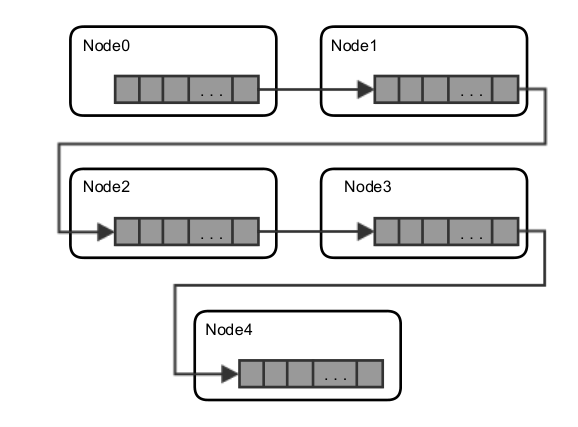
Before the MapReduce execution starts, there is a little pre-elaboration where the global maximum and global minimum of the whole array are retrieved, so to compute the $\mathit{Range}$ of the values in the array.

We now define the behavior of every step. We denote by k1 and v1 respectively the key and the value in input for the Map step; (k2,v2) is the output pair of Map and the input of the Reduce step; (k3,v3) is the output of the Reduce step.

Initialization step

A Source function is performed once on each node to define the (key,value) pairs to be passed to the Map step. More precisely, for every element $i$ of the local array slice, it defines the key k1_i as the global position in the array and the value v1_i as the essential data needed for comparing $i$ with other elements. In this case using “essential data” instead of the whole element is convenient because v1_i might be too heavy to be transferred from a node to another during the intermediate steps. Storing the original position in the key is essential to finally transfer the whole element once its destination has been found.

Map step

This step applies the mapper function to each (local) element $i$ . In particular, the function computes a destination node for the element $i$ , storing it in the output key. Let min be the global minimum; we split the range of values into $N_{\mathit{nodes}}$ intervals, each of size $I=\mathit{Range}/N_{\mathit{nodes}}$ , and we intend to use each node $p$ to host values in the interval

I_{p}=[\mathit{min}+pI,\dots,\mathit{min}+(p+1)I-1]

Then the mapper function takes in input the pair (k1_i,v1_i) and produces the output pair (k2_i,v2_i) where k2 ${}_{i}=q$ for some $q$ such that v1 ${}_{i}\in I_{q}$ , and v2 ${}_{i}=$ (k1_i,v1_i).

Shuffle step

Given the mapper function above, the partition function used in the shuffle step is the identity function. This means that each pair (k2,v2) is sent at node k2. Therefore, since the nodes are ordered, at the end of this step we have that for any pair of nodes $p$ and $q$ , with $p<q$ , all the elements located in $q$ are greater than all the elements located in $p$ . On the other hand the array slices hosted at different nodes are not sorted and in general have different sizes.

Reduce step

As a consequence of the previous steps, at this stage all the pairs hosted at each node share the same key k2. Hence the reducer function is performed once for every different node to sort the local elements with the best algorithm. At the end the local slice of the array is sorted and no elements will be inserted anymore. More precisely, the output of reducer at node j is the pair (k3_j,v3_j), where v3_j is the sorted slice and k3 $j$ its first element.

Sink step

As observed before, the array slices sorted at different nodes have different sizes. The final Sink step, performed once on each node, is then necessary to equally redistribute the sorted array over the nodes. All the sorted sub-arrays will be sent to a specific node, which will take care of the elements redistribution. Notice that the Sink step is logically simple, but involves a huge data transfer between nodes and it is unavoidable.

3.3 Bulk Synchronous Parallel

Compared to MapReduce, BSP is best suited for the analysis of complex, very-large-scale dynamic graphs (billions of nodes, billions of edges). BSP programs consist of a sequence of iterations, called phases, and a set of logical units that communicate by means of message passing. In order to avoid confusion with cluster nodes and actors, we refer to BSP logical units as Agents.

Each phase $S$ is made of the following steps, depicted in Figure 3 where dashed boxes correspond to cluster nodes:

1.

Local computation: parallel agents compute a user-defined function, using their own local memory. The function specifies the behavior of a single agent $V$ in the phase $S$ : it can read messages sent to $V$ in phase $S-1$ , send messages to other agents that will be received at phase $S+1$ , and modify the state of $V$ .
2.

Communication: messages are exchanged between all agents.
3.

Synchronization: each node waits for the others to complete their message transfer at phase $S$ , before starting phase $S+1$ .

In addition, each phase is characterized by a set of initially active agents. These agents execute local computation, then deactivate themselves, and activate other agents by sending a message to them. A job that executes in a BSP machine is defined by a set of agents, a subset of starting active agents, and a stop criterion. A BSP machine stops when there are no more active agents or when the stop criterion is reached even if there are yet active agents.

Figure 3 shows how each agent runs independently and in parallel to the others, both local and remote, but each agent waits for the others at the barrier synchronization, before starting the next phase.

An important part of the analysis of a BSP algorithm rests on quantifying the synchronization and communication that are needed. On the other hand, the BSP agents can be programmed by only focusing on their local memory without directly referring to remote entities.

3.4 Sparse graph exploration with BSP

We now describe how the BSP algorithmic scheme applies to the exploration of a sparse graph. We consider a random directed graph generated with up to 3 edges for every vertex. We assume that each node of the cluster hosts $N$ vertexes, and we let a vertex correspond to a BSP-agent. Every edge can point to a vertex in the same node or to a vertex in a different node, but we assume that the whole graph is simple, that is there are no loops and no more than one edge with the same source and destination.

Each vertex has a parent field and an inbox listing the received messages. The local computation step, executed at every phase by every active vertex, is so defined: the vertex checks the value of its parent field, if it has a non-null value than it deactivates itself, otherwise ( $i$ ) it sets its parent field with the content of the first received message, ( $ii$ ) than it sends a message to every target vertex of any out-coming edge, ( $iii$ ) and finally deactivates itself.

Every vertex that receives a message will be active in the next phase. At the beginning a start vertex is marked as active so to begin the computation. In this problem there is no stop criterion, so the execution stops when there are no more active agents. The parent field and the barrier synchronization between each phase guarantee that each vertex is visited only once, hence the output is a tree. On the other hand, the resulting tree does not contain the vertexes that have not been visited since they were not reachable from the start vertex.

4 Implementation and code style comparison

In this section we comparatively discuss our implementation of the distributed array sorting and the sparse graph exploration problems, both in X10 and Scala+Akka Cluster. First of all, we observe that even if established Big Data application frameworks are available for both technologies (e.g., MR3 for X10 [13] and Spark for Scala [16]), we decided to implement from scratch the MapReduce and BSP frameworks in a lightweight but effective way, so to better value and compare the distinctive features of the two underlying programming models. We assumed for simplicity that the cluster has a fixed number of nodes, and if a node fails we let the whole computation fail. Although Akka is elastic and resilient by nature, and also X10 supports a resilient mode [3], we think that resiliency is orthogonal w.r.t. our goals, and we postpone the comparison of a resilient version of our applications to future work. We also observe that to get best performance with X10 one should use Native X10, which compiles to C++. However we are not interested in absolute performances, we aim instead at drawing some insight about the impact of the concurrency model on the application performances. Hence we rely on Managed X10, which compiles to Java, so to better compare with the Scala+Akka technology.

A first important remark is that, besides the different concurrency models, the two programming platforms under examination significantly differ in their structure. As a consequence, even the programming styles that the developer must adopt, substantially differ. We illustrate below these differences, postponing to Section 5 the experimental comparison.

Project structure

Each one of the four programs is divided in two distinct parts: ( $i$ ) the engine, consisting of the modules that implement the algorithmic scheme (MapReduce or BSP) parametrized w.r.t. the job to be executed, and ( $ii$ ) the job instance (distributed sorting, graph exploration), to be submitted to the engine. This modular structure entails genericity and reusability, and allows a more effective comparison between the two frameworks. The projects based on Akka are formed by a larger number of modules than those in X10. This because Akka entails a more fragmented structure, in which each actor embodies a specific functionality, i.e. a certain role in the project. There are actors representing worker nodes, distinguished actors acting as control nodes, and a number of actors implementing the aggregator pattern to coordinate interactions. Instead, X10 views the cluster at an higher abstraction level than Akka, being able to describe in the same module (i.e. block of code) more computation steps which are usually separated in the most popular programming languages. This is especially possible with the language constructs distinctive of X10: at, async, and finish. In particular, the at construct considerably abstracts and simplifies the distribution of the computation on different nodes. This allows to have a direct view of the distribution to be obtained, which promotes code readability. Moreover, the joint use of these three constructs is very effective in retrieving a value from all nodes or, in general, in the centralized management of the global computation (e.g., in the main classes of the MapReduce and BSP engines).

Main control flow and program launch

The difference in the structure of the two projects is reflected on the main control flow of the programs. In X10 the main control flow is rendered as a control loop that asynchronously spawns code to be executed in every place, while in Akka the control flow is spread on several modules taking advantage of the aggregator pattern.

Even the procedure to launch the program execution reflects the different nature of the two platforms. Starting an X10 execution environment is not so different from starting any other mono-machine program. Basically it requires that an SSH connection is available between all the machines, then a start-up script, provided by the framework, activates all the nodes. The script basically requires only two parameters: the number of places to be activated, and an IP address list of the available machines. If the number of places is greater than the number of IP addresses, then more than one place will be activated on some machines. This start mode allows to easily execute the program in batch mode, which will be required by our tests, as we shall see in the next section.

Akka Cluster has instead a dynamic and decentralized view of the cluster, which makes the startup more complex. There is more than one way to boot the whole system, however, in order to start the tests in batch mode, a script has been developed to have a centralized boot of the system. The script requires an “ip:port” list in order to know where to place the Akka nodes, and an SSH connection available between all the machines. The script connects to the machines and boots up every single node.

Data structures

Being distributed by nature, X10 has some built-in useful distributed data structures. In this case, DistArray represents a generic multidimensional array distributed over some places, and provides a centralized control of the array. For instance, the class has the method localIndices that returns a subset of array’s indexes accessible from the place where it has been called; remind that all the other indexes cannot be accessed from that place. To illustrate, the following code retrieves the maximum value of the whole distributed array. In the second line, the finish keyword waits for the termination of all the asynchronous activities into the inner block. In the third line, an asynchronous activity is started in every place. Then, in each place, the maximum is retrieved among the local values and is returned to the asynchronous call. At last, when the finish is satisfied, the MaxReducer is evaluated and the maximum value is stored to the max value.

val max =
    finish(Reducible.MaxReducer[Long](Long.MIN_VALUE)){
       for(p in Place.places()) at(p) async {
          var localMax:Long = Long.MIN_VALUE;
          for (i in originArray.localIndices())
            if (originArray(i) > localMax)
               localMax = originArray(i);
          offer localMax;
       }
};

This piece of code also clearly shows how the control flow can be managed in X10 within few lines.

Akka design states that every node is independent and there must not be a single-point of failure, therefore there is no distributed data structure spanning over the nodes, but it is required to independently manage individual slices on every node. In the case of the distributed array, we let DistArrayNodeActor hold, in every node, a slice of the distributed array and manage all the operations on it. As to retrieve the global maximum/minimum of the whole array, a MinMaxAggregator actor is instantiated, so that it asks to the worker nodes the maximum/minimum of their local slice. Then the actor collects the responses and extracts the global maximum/minimum.

As for the distributed graph processed by BSP, each node holds its local vertexes in an array of size $N$ , and each vertex holds in turn an array of three remote references to other vertexes, that represent the edges of the graph.

The cost of communication

In Section 3.3 we have seen that the second step of the BSP algorithm involves message transfer between all agents. This communication step is accomplished in X10 by storing the list of received messages directly into the (possibly remote) recipient. Since X10 is a language with a shared memory model, and the insertion of messages in this list is allowed to all the active agents at the current phase, it is necessary to control the insertion of messages in the list with an atomic block.

Although the atomic block is an heavy construct ([12]), in this case its use is appropriate, given the enormous number of possible senders. Other solutions, such as a memory slot for each possible incoming message, are inapplicable. We observe that the Shuffle and Sink steps of MapReduce do not suffer from the same problem since in their case the possibility of predicting the target destination of the involved communications allows to reserve a reasonable amount of memory slots to be filled without resorting to atomic.

In the Akka-based implementation, the BSP-inbox of an agent is implemented with an actor, MessageReceiver, to which is delegated the function of receiving messages. The code of MessageReceiver is reported below: collects in a single block all messages received in a given phase (5th line) to be returned to the agent in the next phase (8th line):

class MessageReceiver[S] extends Actor {
  val inc = Array(ArrayBuffer.empty[Any], ArrayBuffer.empty[Any])
  def receive = {
    case Message(phase, x) => inc(phase%2) += x
      sender() ! MsgReceived

    case GetInbox(phase) =>
      sender() ! inc(phase%2).toArray
      inc(phase%2).clear()
 }
}

As a final remark about Akka’s communication model, we observe that Akka does not impose constraints on the size of the messages exchanged between the actors, that is, the messages within the same actor system can have any size. However, the connections between the cluster nodes are based on Akka Remote that uses the UDP protocol, which in turn does not support arbitrary large datagrams. Therefore, large messages such as those exchanged in the Sink step of the MapReduce projects, have to be chunked, and then re-compacted, by the programmer.

Local and remote parallelism

In the implementations of MapReduce we decided to focus on remote parallelism, hence each node just hosts sequential computation. More precisely, all the local executions of the mapper functions (one for each local array element) run sequentially, and the reducer function is performed once for each node. Each step of the algorithm is then executed in parallel at the level of cluster nodes.

On the other hand, in the BSP implementations we studied both local and remote parallelization opportunities. In particular, observe that the local computation involved in the first step of each BSP phase can be parallelized (see Figure 3). Indeed, in our Akka implementation, each agent executes in parallel; remind that we let $N$ agents run on each node. On the other hand, when $N$ grows, X10 does not properly scale-up: as we shall see in the next section, X10 executions with a large number of agents per node ( $N\!>\!4000$ ) give rise to a runtime warning saying that they are running too many threads, and execution does not terminate. We will more precisely discuss this issue in Section 5, we just observe here that the problem comes form the usage of the atomic construct, whose implementation blocks both the lightweight activity, i.e., the logical task, and the underlying worker thread ([12]). We thus developed two X10 versions of BSP: X10P, where local agents are executed in parallel, and X10S, where agents in the same node are executed sequentially. Anyway, notice that the atomic block described above is necessary even in the case where the local agents are sequentially run, since local agent runs in parallel to agents in other places.

4.1 Comparison of models

We conclude this section by summarizing the comments above into a more general picture. Our detailed description of the four applications illustrates the very different programming styles involved by X10 and Scala. Such a difference reflects the fact the design principles of these languages significantly diverge, despite being both very expressive.

As far as X10 is concerned, even if functional constructs are available and the async construct greatly simplifies asynchronous execution, the underlying shared-memory model and the centralized control of the distributed computation bring about an imperative programming style with critical accesses to shared memory. In this sense X10 is predisposed to a more synchronous programming, where concurrency involve (large) sets of activities running in parallel with few coordination requests. Accordingly, we will see in the next section that X10 shines on the MapReduce application, which essentially consists of sequences of steps with inter-node parallelism.

In Scala, sticking to the actor model is a choice, since shared variables are still available. For instance, using the futures requires the operations scheduled at the future completion not to modify the internal state of the actor so to prevent interferences. However, the functional flavour of the language promotes the definition of well-defined behaviours to be delegated and composed by means of actors and futures. Such a disaggregation suits a dynamic and decentralized view of the cluster, which fosters the distributed execution of asynchronous operations boosting the parallelism. Accordingly, we will see that Akka’s asynchronous programming style shines on the scale-up, that is in presence of intra-node concurrency, where a large number of concurrent activities can be effectively coordinated without the constraints and the limitations of synchronization constructs.

5 Experimental comparison

In this section we provide the details of our experimental comparison, and we discuss the execution performances of the projects under consideration.

To develop the four projects we used the following tools: X10 language (v. 2.5.1) and X10 Development Tool IDE (v. 2.5.1) for X10 projects, and Scala language (v. 2.11.4), Akka-actor (v. 2.3.8), Akka-remote (v. 2.3.8), Akka-cluster (v. 2.3.8), IntelliJ IDEA IDE (v. 14.0.2) and Scala Build Tool (v. 0.3.7) for Akka projects. To perform the tests we used the cluster of the Department of Mathematics of the University of Padova. The table below lists the machines we used, each one with the following minimum requirements: 8 cores, 16GB RAM, Infiniband connection, and JVM 1.6 (OpenJDK).

\begin{array}[]{ r l r }\hline\cr\hline\cr\#&\text{CPU}&\text{RAM}\\ \hline\cr 1&\text{2 x Quad-Core Intel(R) Xeon(R) X5460 @ 3.16GHz}&\text{32GB}\\ 2&\text{2 x Quad-Core Intel(R) Xeon(R) E5520 @ 2.27GHz}&\text{32GB}\\ 3&\text{2 x Quad-Core Intel(R) Xeon(R) E5520 @ 2.27GHz}&\text{32GB}\\ 4&\text{2 x Quad-Core Intel(R) Xeon(R) E5520 @ 2.27GHz}&\text{32GB}\\ 5&\text{2 x Six-Core Intel(R) Xeon(R) X5650 @ 2.67GHz}&\text{64GB}\\ 6&\text{2 x Quad-Core Intel(R) Xeon(R) X5460 @ 3.16GHz}&\text{16GB}\\ 7&\text{2 x Quad-Core Intel(R) Xeon(R) E5520 @ 2.27GHz}&\text{32GB}\\ 8&\text{2 x Quad-Core AMD Opteron(tm) 2378 @ 2.40GHz}&\text{64GB}\\ 9&\text{2 x Quad-Core Intel(R) Xeon(R) E5520 @ 2.27GHz}&\text{32GB}\\ 10&\text{2 x Eight-Core Intel(R) Xeon(R) E5-2680 @ 2.70GHz}&\text{256GB}\\ \hline\cr\hline\cr\end{array}

The access to the cluster is regulated by the Torque Resource Manager queuing system, which defines the framework for the aggregate use. To use the cluster it is then necessary to submit to the queuing system an executable that specifies the resource requirements in terms of the number of required machines and the number of required cores for each machine; then Torque starts the program execution by assigning an IP address to each required core, depending on the current load of the system. When more than one core per machine has been requested, the same IP address will be assigned multiple times.

As anticipated in Section 4, the X10 platform provides a script which, given the list of IP addresses, launches the executable on each machine and autonomously establishes the connections between the nodes (i.e. X10 places). Akka instead requires a manual script that computes the various “ip:port” combinations and starts each node separately. This works well, given the relatively small size we achieved; for larger clusters (200, 1000, or more nodes), we would have to load the nodes interactively, and adapt the configuration of the gossip protocol.

In the case of X10, a place then corresponds to a JVM, and similarly, an Akka node corresponds to a single JVM.

Description of the experiments

Given the random generation of the problems and the intrinsic nondeterminism, the reported results reflect the average time of ten executions for each instance. The small variability revealed by the execution times of the same instance is an indication of the reliability of the obtained results.

To measure the performance of programs, we first considered varying the problem size, then varying the number of nodes in the cluster. From now on, when we consider the number of nodes in the cluster, we will use the notation $A$ x $B$ , where $A$ is the number of physical machines used, and $B$ is the number of nodes on that machine. This to highlight that part of the communication between nodes can take place within the same machine and does not pass through a real network, which is clearly slower.

It is important to observe that, besides the cluster size, in the performance analysis it is crucial to consider the single machine load. For instance, a cluster 8x4 is very different from a cluster 4x8: they have the same number of nodes, but with a different distribution between the machines, leading to different performances (as illustrated by the plots in the following subsection). More precisely, since most of the machines have eight cores, a machine hosting eight nodes, such as those in the 4x8 cluster, is somehow “saturated”. Instead, when just four nodes run on a eight-core machine, the corresponding four JVMs enjoy more powerful resources. This key observation highlights the fact that in a performance comparison it is not enough to consider just the number of nodes in the cluster, but also the available resources guaranteed by the machines hosting the nodes.

5.1 MapReduce

Figure 4: MapReduce - Variation of the array size on 10x3 nodes.

Variation of the array size

Figure 4 shows the execution times of Akka and X10 on the MapReduce implementation in a cluster where the number of nodes is fixed (10x3), while the size of the array varies from $10^{3}$ to $10^{6}$ integers. What you notice is that Akka is a bit slower than X10 in all the considered cases. Remind that in our implementation the local computation is sequential, hence the program is locally synchronous. We then think that the difference in the performances comes from Akka’s overhead due to asynchronous message exchange.

Figure 5: MapReduce - Variation of the cluster size with an array of

10^{6}

elements.

Variation of the cluster size

The plot in Figure 5 shows the comparison made by keeping constant the array size (set to $10^{6}$ elements), while varying the number of nodes in the cluster. Also in this case Akka is a bit slower, in a uniform manner, compared to X10. Notice in particular the central gap between the execution times in a 8x4 and a 4x8 cluster: both programs have better performances on “non-saturated” machines. More generally, what emerges is that both languages very well succeed in managing the change in the number of nodes, but the divergent directions of the segments might suggest that X10 scales-out better than Akka for larger clusters. However, the considerations made above about the saturation of the machines indicate that no proper scale-out considerations can be done without further tests. For instance, the divergence of Akka might as well be explained again by the overhead of the asynchronous management of messages, aggravated by the machine saturation.

5.2 Bulk Synchronous Parallel

\begin{array}[]{ l | *{6}{r} }\hline\cr\hline\cr\text{\#Agents}&500&1^{\mbox{${\cdot}$}}000&2^{\mbox{${\cdot}$}}000&4^{\mbox{${\cdot}$}}000&8^{\mbox{${\cdot}$}}000&16^{\mbox{${\cdot}$}}000\\ \hline\cr\text{Akka}&4.261&6.118&7.939&11.467&15.178&24.947\\ \text{X10P}&3.616&5.199&7.406&12.487&{}^{*}21.271&\text{N/A}\\ \text{X10S}&4.029&6.175&10.201&18.660&37.628&67.718\\ \hline\cr\hline\cr\end{array}

Figure 6: BSP - Variation of agents per node on a cluster with 8x4 nodes.

Variation of the number of agents per node

As we said in Section 4, we developed two X10 versions of BSP: X10P, where local agents are executed in parallel, and X10S, where agents in the same node are executed sequentially. Although X10P can’t handle all tested instances, it is reported to actually compare X10 and Akka on the algorithm with the same degree of parallelism at least on those instances in which X10P properly terminates.

Figure 6 shows a comparison of the implementations of the BSP model, considering a cluster of constant size ( $8$ x $4$ ), where the variation is made on the number of agents per node. The plot and the table below with detailed time results, highlight how Akka is slightly slower for small instances, however its asynchronous model becomes more efficient in large instances, because it avoids bottlenecks caused by the use of atomic. Also observe that the locally sequential version X10S is very slow, because it does not exploit the parallel execution of the independent agents. The X10P case is the most efficient in smallest instances, where concurrency on shared variables is lower, while it is worse than Akka when the concurrency increases.

The point in the plot labeled by $X$ , that is the X10P instance with $8000$ agents per node, corresponds to the average between only two iterations (instead of ten), since the other eight failed by suspending with a “too many threads” warning. Instead, in the case of $16000$ agents per node, no execution succeeded.

Variation of the cluster size

The plot in Figure 7 considers the variation of the cluster size in BSP assuming a graph with $4000$ agents per node. Also in this experiment we distinguish the case of saturated and non-saturated machines. In the tests with non-saturated machines the executions of X10P and Akka last substantially the same time. X10S is instead proportionally slower than the others, again because of the lack of local parallelism.

On the other hand, on saturated machines, that is in the rightmost part of the plot, there is a noticeable deterioration of execution times. Observe that in this case Akka’s performances are always in between those of X10P and X10S, however the lack of linearity in the results indicates that it is important to consider, also in this case, the saturation of the machines. As for X10P executions, one iteration failed in the cases 6x4 and 6x8 (labeled with $X$ ), while four iterations failed in cases 4x8 and 8x8 (labeled with $Y$ ); this is a sign that the termination is not guaranteed.

\begin{array}[]{ l | *{6}{r} }\hline\cr\hline\cr\text{\#Nodes}&\text{4x4}&\text{5x4}&\text{6x4}&\text{7x4}&\text{8x4}\\ \hline\cr\text{Akka}&14.248&14.530&16.656&16.319&16.125\\ \text{X10S}&31.831&35.507&36.801&39.560&40.693\\ \hline\cr\hline\cr\end{array}

\begin{array}[]{ l | *{6}{r} }\hline\cr\hline\cr\text{\#Nodes}&\text{4x8}&\text{5x8}&\text{6x8}&\text{7x8}&\text{8x8}\\ \hline\cr\text{Akka}&25.787&25.490&25.665&28.116&28.043\\ \text{X10S}&47.097&51.036&51.935&53.704&58.379\\ \hline\cr\hline\cr\end{array}

Figure 7: BSP - Variation of the cluster size with

4000

agents per node.

In order to fully test Akka’s scalability, we also tested the BSP program by assuming a graph with $10^{4}$ agents per node and varying the cluster size. As illustrated by the execution times reported in the table in Figure 7, Akka’s implementation scales with the size of the cluster and the corresponding increase of the number of total agents. This then means that it scales well with the proliferation of messages exchanged in the system. The table also shows that the execution time increase of X10S is sharper, on the other hand, no X10P execution terminated.

5.3 Performance analysis

In the light of what emerged from the performance comparison, we have that X10 excels with inter-node parallelism, while Akka shines on intra-node concurrency. It is important to remind here that fair performance tuning X10 applications requires different strategies (see [17]), such that avoiding the atomic construct and relying on Native X10 which compiles to C++. Nevertheless, the main explanation of these results essentially comes from the underlying programming models, as observed in Section 4, which are indeed the main target of our investigation.

X10’s centralized control appears to be best suited to inter-node parallelism, hence to algorithms, like MapReduce, characterized by sequences of independent steps with rare and predictable synchronizations that minimize the need to protect the access to shared memory. Instead, Akka makes the most of his asynchronous model in presence of a high degree of concurrent activities, that can be efficiently coordinated with no need of blocking mechanisms.

Let’s consider this point more in depth: observe that both Akka and X10 distinguish logical tasks (respectively the actors in Akka and the activities in X10) from the worker threads, so to allow the execution of many tasks with a few threads. However, in the two programming models such a distinction has a very different impact. Indeed, consider how the X10 runtime realizes the decoupling between tasks and worker threads: if a thread is about to block because of a pending synchronization such as an atomic block, before suspending it starts a new worker thread with the aim of preserving the parallelism. However the system has a limit (set by default to $1000$ threads), after which the user is warned with the already seen “too many threads” message. Instead in the asynchronous model of actors the tasks never block, hence worker threads can be mainly reused making the best of the initial pool of threads. Moreover, [8] illustrates how the functional model provides opportunities to further improve the decoupling between logical tasks and worker threads by means of the continuation-passing style. Anyway, despite the non-blocking implementation strategies, synchronous primitives like atomic, are also logical blockers that establish a conceptual limit to the scale-up: if a shared variable undergoes many synchronized accesses, any task that needs to access must wait his turn, so the global computation hardly advance. This is indeed what happens in the inbox of the BSP-agents, where a huge number of senders is ready to deliver a message but few tend to do it.

6 Conclusions

In this paper we compared concrete implementations of the MapReduce and BSP algorithmic schemes using the X10 and Akka Cluster platforms. Rather than addressing performance issues, we aimed at testing the actor model and the shared memory model at work on a Big Data Analytics scenario. The experimental tests assess the expected conceptual scale-up limit entailed by the blocking constructs required to safely access shared memory. Moreover, both the code style comparison and the experimental results, attest that the centralized and imperative flavour of X10 stands out in the MapReduce implementation, while Akka’s actors foster the distributed execution of asynchronous tasks better scaling to the higher concurrency degree required by BSP.

As for the scale-out, we showed that both platforms can properly handle executions that involve up to 64 nodes. However, a more faithful analysis requires additional tests with a larger cluster and carefully tuning the resources available in each machine; this kind of analysis is the subject of future work. We also plan to extend our investigation to assess the impact of the programming models on fault tolerant executions. Resiliency is indeed a critical issue of Big Data applications and both X10 and Akka provide support for resilient executions. In this case however it is necessary to suitably structure the problems in order to evaluate the fault tolerance potential of the two platforms.

References

[1] R. H. Bisseling and W. F. McColl. Scientific computing on bulk synchronous parallel architectures. In Proc. of IFIP 13th World Computer Congress:(1), pages 509–514, 1994.
[2] P. Charles, C. Grothoff, V. Saraswat, C. Donawa, A. Kielstra, K. Ebcioglu, C. von Praun, and V. Sarkar. X10: An object-oriented approach to non-uniform cluster computing. In Proc. of OOPSLA’05, pages 519–538, 2005. ACM.
[3] D. Cunningham, D. Grove, B.Herta, A.Iyengar, K. Kawachiya, H. Murata, V. Saraswat, M. Takeuchi, and O.Tardieu. Resilient X10: efficient failure-aware programming. In Proc. of PPoPP ’14, pages 67-80, 2014. ACM.
[4] G. Czajkowski, M. Dvorský, J. Zhao, and M. Conley. Sorting petabytes with MapReduce - the next episode. http://googleresearch.blogspot.com/2011/09/sorting-petabytes-with-mapreduce-next.html, 2011.
[5] J. Dean and S. Ghemawat. Mapreduce: simplified data processing on large clusters. In Proc. of OSDI’04:(6), pages 10-10. USENIX Association, 2004.
[6] K. Ebcioglu, V. Saraswat, and V. Sarkar. X10: Programming for hierarchical parallelism and non-uniform data access. In Proceedings of the International Workshop on Language Runtimes, OOPSLA, 2004.
[7] M. T. Goodrich, N. Sitchinava, and Q. Zhang. Sorting, searching, and simulation in the mapreduce framework. In Algorithms and Computation: (7074), pages 374–383. Springer Berlin Heidelberg, 2011.
[8] P. Haller and M. Odersky Scala Actors: Unifying thread-based and event-based programming. Theoretical Computer Science: 410(2-3), pages 202-220, 2009.
[9] T. Kajdanowicz, P. Kazienko, and W. Indyk. Parallel processing of large graphs. CoRR, abs/1306.0326, 2013.
[10] D. Krizanc and A. Saarimaki. Bulk synchronous parallel: Practical experience with a model for parallel computing. In Proc. of PACT ’96, pages 208-217, 1996. IEEE Computer Society.
[11] G. Malewicz, M. H. Austern, A. J. Bik, J. C. Dehnert, I. Horn, N. Leiser, and G. Czajkowski. Pregel: A system for large-scale graph processing. In Proc. of SIGMOD ’10, pages 135–146, 2010. ACM.
[12] V. Saraswat, O.Tardieu, D. Grove, D. Cunningham, M. Takeuchi and B. Herta. A Brief Introduction To X10. http://x10.sourceforge.net/documentation/intro/latest/html/, 2014.
[13] A. Shinnar, D. Cunningham, V. Saraswat, and B.Herta. M3R: increased performance for in-memory Hadoop jobs. In Proc. of the VLDB Endowment, 5(12), pages 1736–1747, 2012.
[14] J. D. Ullman. Designing good mapreduce algorithms. XRDS, 19(1):pages 30–34, Sept. 2012. ACM.
[15] L. G. Valiant. A bridging model for multi-core computing. Journal of Computer and System Sciences: 77(1), pages 154–166, Jan. 2011.
[16] M. Zaharia, M. Chowdhury, M. J. Franklin, S. Shenker, and I. Stoica. Spark: Cluster computing with working sets. In Proc. of HotCloud’10, pages 10–10, 2010. USENIX Association.
[17] X10 Performance Tuning http://x10-lang.org/documentation/practical-x10-programming/performance-tuning.html

Actors vs Shared Memory: two models at work on Big Data application frameworks

Abstract

1 Introduction

Structure of the paper

2 The programming platforms

3 Two BigData algorithmic schemes

3.1 MapReduce

3.2 Sorting a distributed array with MapReduce

Initialization step

Map step

Shuffle step

Reduce step

Sink step

3.3 Bulk Synchronous Parallel

3.4 Sparse graph exploration with BSP

4 Implementation and code style comparison

Project structure

Main control flow and program launch

Data structures

The cost of communication

Local and remote parallelism

4.1 Comparison of models

5 Experimental comparison

Description of the experiments

5.1 MapReduce

Variation of the array size

Variation of the cluster size

5.2 Bulk Synchronous Parallel

Variation of the number of agents per node

Variation of the cluster size

5.3 Performance analysis

6 Conclusions

References

Actors vs Shared Memory: two models at work
on Big Data application frameworks