Removing systematic errors for exoplanet search via latent causes
Abstract
We describe a method for removing the effect of confounders in order to reconstruct a latent quantity of interest. The method, referred to as half-sibling regression, is inspired by recent work in causal inference using additive noise models. We provide a theoretical justification and illustrate the potential of the method in a challenging astronomy application.
Keywords:
machine learning, ICML, causal inference, confounder, systematics, systematic error, exoplanet, astronomy, regression1 Introduction
The present paper proposes and analyzes a method for removing the effect of confounding noise. The analysis is based on a hypothetical underlying causal structure. The method does not infer causal structures; rather, it is influenced by a recent thrust to try to understand how causal structures facilitate machine learning tasks (Schölkopf et al., 2012).
Causal graphical models as pioneered by Pearl (2000); Spirtes et al. (1993) are joint probability distributions over a set of variables , along with directed graphs (usually, acyclicity is assumed) with vertices , and arrows indicating direct causal influences. By the causal Markov assumption, each vertex is independent of its non-descendants, given its parents.
There is an alternative view of causal models, which does not start from a joint distribution. Instead, it assumes a set of jointly independent noise variables, one for each vertex, and a “structural equation” for each variable that describes how the latter is computed by evaluating a deterministic function of its noise variable and its parents. This view, referred to as a functional causal model (or nonlinear structural equation model), leads to the same class of joint distributions over all variables (Pearl, 2000; Peters et al., 2014), and we may thus choose either representation.
The functional point of view is useful in that it often makes it easier to come up with assumptions on the causal mechanisms that are at work, i.e., on the functions associated with the variables. For instance, it was recently shown (Hoyer et al., 2009) that assuming nonlinear functions with additive noise renders the two–variable case identifiable — i.e., a case where conditional independence tests do not provide any information, and it was thus previously believed that it is impossible to infer the structure of the graph based on observational data.
In this work we start from the functional point of view and assume the underlying causal graph shown in Fig. 1. Here, are jointly random variables (RVs) (i.e., RVs defined on the same underlying probability space), taking values denoted by . We do not require the ranges of the random variables to be , in particular, they may be vectorial. All equalities regarding random variables should be interpreted to hold with probability one. We further (implicitly) assume the existence of conditional expectations.
Note that while the causal motivation was helpful for our work, one can also view Fig. 1 as a DAG (directed acyclic graph) without causal interpretation, i.e., as a directed a graphical model. We need and (and in some cases also ) to be independent, which follows from the given structure no matter whether one views this as a causal graph or as a graphical model.
2 Half-Sibling Regression
Suppose we are interested in the quantity , but unfortunately we cannot observe it directly. Instead, we observe , which we think of as a degraded version of that is affected by noise . Clearly, without knowledge of , there is no way to recover . However, we assume that also affects another observable quantity (or a collection of quantities) . By the graph structure, conditional on , the variables and are dependent (in the generic case), thus contains information about . This situation is quite common if and are measurements performed with the same apparatus, introducing the noise . In the physical sciences, this is often referred to as systematics, to convey the intuition that these errors are not simply due to random fluctuations, but caused by systematic influences of the measuring device. In our application below, both types of errors occur, but we will not try to tease them apart. Our method addresses errors that affect both and , for instance by acting on , no matter whether we call them random or systematic.
How can we use this information in practice? Unfortunately, without further restrictions, this problem is still too hard. Suppose that randomly switches between , where (Schölkopf et al., 2012). Define the structural equation for the variable as follows: , where are distinct functions that compute from — in other words, we randomly switch between different mechanisms. Clearly, no matter how many pairs we observe, we can choose a sufficiently large along with functions such that there is no way of gleaning any reliable information on from the — e.g., there may be more than there were data points. Things could get even worse: for instance, could be real valued, and switch between an uncountable number of functions. To prevent this kind of behavior, we need to simplify the way in which is allowed to depend on .
Before we do so, we need to point out a fundamental limitation. The above example shows that it can be arbitrarily hard to get information about from finite data. However, even from infinite data, only partial information is available and certain ‘‘gauge’’ degrees of freedom remain.11 1 This means that there are some degrees of freedom in the parametrization of the model which do not affect the observable model. In particular, given a reconstructed , we can always construct another one by applying an invertible transformation to it, and incorporating its inverse into the function computing from and . This includes the possibility of adding an offset, which we will see below.
We next propose an assumption which allows for a practical method to solve the problem of reconstructing up to the above gauge freedom. The method is surprisingly simple, and while we have not seen it in the same form elsewhere, we do not want to claim originality for it. Related tricks are occasionally applied in practice, often employing factor analysis to account for confounding effects (Price et al., 2006; Yu et al., 2006; Johnson & Li, 2007; Kang et al., 2008; Stegle et al., 2008; Gagnon-Bartsch & Speed, 2011). We will also present a theoretical analysis that provides insight into why and when these methods work.
2.1 Complete Information
Inspired by recent work in causal inference, we use nonlinear additive noise models (Hoyer et al., 2009). Specifically, we assume that there exists a function such that
| (1) |
Note that we could equally well assume the more general form , and the following analysis would look the same. However, in view of the above remark about the gauge freedom, this is not necessary since can at most be identified up to a (nonlinear) reparametrization anyway. Note, moreover, that while for Hoyer et al. (2009), the input of is observed and we want to decide if it is a cause of , in the present setting the input of is unobserved (Janzing et al., 2009), and the goal is to recover , which for Hoyer et al. (2009) played the role of the noise.
The intuition behind our approach is as follows. Since , cannot predict , and thus neither ’s influence on . It may contain information, however, about the influence of on , since is also influenced by . Now suppose we try to predict from . As argued above, whatever comes from cannot be predicted, hence only the component coming from will be picked up. Trying to predict from is thus a vehicle to selectively capture ’s influence on , with the goal of subsequently removing it, to obtain an estimate of referred to as :
Definition 1
| (2) |
For an additive model (1), our intuition can be formalized: in this case, we can predict the additive component in coming from — which is exactly what we want to remove to cancel the confounding effect of and thus reconstruct (up to an offset):
Proposition 1
Suppose are jointly random variables, and is a measurable function. If there exists a function such that
| (3) |
i.e., can in principle be predicted from perfectly, then we have
| (4) |
If, moreover, the additive model assumption (1) holds, with RVs on the same underlying probability space, and , then
| (5) |
In our main application below, will be systematic errors from an astronomical spacecraft and telescope, will be a star under analysis, and will be a large set of other stars. In this case, the assumption that has a concrete interpretation: it means that the device can be self-calibrated based on measured science data only (Padmanabhan et al., 2008).
Proof.
Due to (3), we have
| (6) |
Proposition 1 provides us with a principled recommendation how to remove the effect of the noise and reconstruct the unobserved up to its mean : we need to subtract the conditional expectation (i.e., the regression) from the observed (Definition 1). The regression can be estimated from observations using (linear or nonlinear) off-the-shelf methods. We refer to this procedure as half-sibling regression to reflect the fact that we are trying to explain aspects of the child by regression on its half-sibling(s) in order to reconstruct properties of its unobserved parent .
Note that is a function of , and is the random variable . Correspondingly, (4) is an equality of RVs. By assumption, all RVs live on the same underlying probability space. If we perform the associated random experiment, we obtain values for and , and (4) tells us that if we substitute them into and , respectively, we get the same value with probability 1. Eq. (5) is also an equality of RVs, and the above procedure therefore not only reconstructs some properties of the unobservable RV — it reconstructs, up to the mean , and with probability 1, the RV itself. This may sound too good to be true — in practice, of course its accuracy will depend on how well the assumptions of Proposition 1 hold.
If the following conditions are met, we may expect that the procedure should work well in practice:
(i) should be (almost) independent of — otherwise, our method could possibly remove parts of itself, and thus throw out the baby with the bathtub. A sufficient condition for this to be the case is that be (almost) independent of , which often makes sense in practice, e.g., if is introduced by a measuring device in a way independent of the underlying object being measured. Clearly, we can only hope to remove noise that is independent of the signal, otherwise it would be unclear what is noise and what is signal. A sufficient condition for , finally, is that the causal DAG in Fig. 1 correctly describes the underlying causal structure.
Note, however, that
Proposition 1
and thus our method also applies if , as long as .
(ii)
The observable is chosen such that can be predicted as well as possible from it; i.e., contains enough information about and, ideally, acts on both and in similar ways such that a “simple” function class suffices for solving the regression problem in practice.
This may sound like a rather strong requirement, but we will see that in our astronomy application, it is not unrealistic: will be a large vector of pixels of other stars, and we will use them to predict a pixel of a star of interest. In this kind of problem, the main variability of will often be due to the systematic effects due to the instrument also affecting other stars, and thus a large set of other stars will indeed allow a good prediction of the measured .
Note that it is not required that the underlying structural equation model be linear — can act on and in nonlinear ways, as an additive term .
In practice, we never observe directly, and thus it is hard to tell whether the assumption of perfect predictability of from holds true. We now relax this assumption.
2.2 Incomplete Information
First we observe that is a good approximation for whenever is almost determined by :
Lemma 2
For any two jointly random variables , we have
| (9) |
Here, is the random variable with , and is the random variable with . Then (9) turns into
| (10) |
Proof.
Note that for any random variable we have
by the definition of variance, applied to the variable . Hence
where both sides are functions of . Taking the expectation w.r.t. on both sides yields
where we have used the law of total expectation on the right hand side. ∎
This leads to a stronger result for our estimator (2):
Proposition 3
Let be measurable, jointly random variables with , and . The expected squared deviation between and satisfies
| (11) |
Proof.
The result follows using Lemma 2 with . ∎
Note that Proposition 1 is a special case of Proposition 3: if there exists a function such that , then the r.h.s. of (11) vanishes. Proposition 3 drops this assumption, which is more realistic: consider the case where , where is another random variable. In this case, we cannot expect to reconstruct the variable from exactly.
There are, however, two settings where we would still expect good approximate recovery of :
(i) If the standard deviation of goes to zero, the signal of in becomes strong and we can approximately estimate from , see Proposition 4.
(ii) Alternatively, we observe many different effects of . In the astronomy application below, and are stars, from which we get noisy observations and . Proposition 5 below shows that observing many different helps reconstructing , even if all depend on through different functions and their underlying (independent) signals do not follow the same distribution. The intuition is that with increasing number of variables the independent “average” out, and thus it becomes easier to reconstruct the effect of .
Proposition 4
Assume that and let
where , and are jointly independent, , , , and is invertible. Then
where .
Proof.
We have for that
for some that is bounded in (the implications follow from the continuous mapping theorem).22 2 The notation denotes convergence in probability with respect to the measure of the underlying probability space. This implies
because
( convergence follows because is bounded). But then
∎
Proposition 5
Assume that and that satisfies
where all , and are jointly independent, , , for all , and
is invertible with uniformly equicontinuous. Then
where we define .
Proof.
By Kolmogorov’s strong law, we have for
that
for some that are uniformly bounded in (the implication follows from uniform equicontinuity, implication by the continuous mapping theorem). This implies
because
(The convergence of the right hand side follows from and boundedness of ). But then
∎
The next two subsections discuss optional extensions of our approach. Readers who are mainly interested in the application may prefer to move to Section 3 directly.
2.3 Time Series
Above, we have worked with random variables and assumed that the regression is performed on i.i.d. data drawn from those random variables. However, in practice we also encounter problems where the data are drawn from random processes depending on time.
Consider a causal graph with an additional confounder representing time, see Figure 2, and assume that the signals and have a time series structure. This representation becomes necessary if and share a strong periodicity, for example. If we want to retain this periodicity, we should not simply regress on .
In many applications the signals may have a time structure but we expect and as well as and to be independent. We further assume that the signals and will normally not share any strong frequencies. In those situations the representation shown in Figure 3 may be more appropriate.
Because of the independence between and , we can proceed as before and estimate as the residuals after regressing from (we could even allow to have a time structure, too). The graph structure shows that after including as a predictor for , all other may contain further information about . Note however, that this dependence decreases quickly with increasing , especially when the contribution of to is small compared to the contribution of to . Still, in some simulation settings, including different time lags into the model for improves the performance of the method (in terms of reconstructing ) compared to predicting only from (results not shown). We expect that identifiability statements similar to the i.i.d. case may hold (see sections 2.1 and 2.2).
2.4 Prediction from Non-Effects of the Noise Variable
While Fig. 1 shows the causal structure motivating our work, our method does not require a directed arrow from to — it only requires that , to ensure that contains information about . We can represent this by an undirected connection between the two (Fig. 4), and note that such a dependence may arise from an arrow directed in either direction, and/or another confounder that influences both and . This confounder need not act deterministically on , hence effectively removing our earlier requirement of a deterministic effect, cf. (1).
3 Applications
3.1 Synthetic Data
We analyze two simulated data sets that illustrate the identifiability statements from Sections 2.1 and 2.2.
Increasing relative strength of in a single .
We consider instances (each time we sample i.i.d. data points) of the model and , where and are randomly chosen sigmoid functions and the variables , and are normally distributed. The standard deviation for is chosen uniformly between and , the standard deviation for is between and . Because can be recovered only up to a shift in the mean, we set its sample mean to zero. The distribution for , however, has a mean that is chosen uniformly between and and its standard deviation is chosen from the vector . Proposition 4 shows that with decreasing standard deviation of we can recover the signal . Standard deviation zero corresponds to the case of complete information (Section 2.1). For regressing on , we use the function gam (penalized regression splines) from the R-package mgcv; Figure 5 shows that this asymptotic behavior can be seen on finite data sets.
Increasing number of observed variables.
Here, we consider the same simulation setting as before, this time simulating for . We have shown in Proposition 5 that if the number of variables tends to infinity, we are able to reconstruct the signal . In this experiment, the standard deviation for and is chosen uniformly between and ; The distribution of is the same as above. It is interesting to note that even additive models (in the predictor variables) work as a regression method (we use the function gam from the R-package mgcv on all variables and its sum ). Figure 5 shows that with increasing the reconstruction of improves.


3.2 Exoplanet Light Curves
The field of exoplanet search has recently become one of the most popular areas of astronomy research. This is largely due to the Kepler space observatory launched in 2009. Kepler observed a tiny fraction of the Milky Way in search of exoplanets. The telescope was pointed at same patch of sky for more than four years (Fig. 6 and 7). In that patch, it monitored the brightness of 150000 stars (selected from among 3.5 million stars in the search field), taking a stream of half-hour exposures using a set of CCD (Charge-Coupled Device) imaging chips arranged in its focal plane using the layout visible in Fig. 7.


Kepler detects exoplanets using the transit method. Whenever a planet passes in front of their host star(s), we observe a tiny dip in the light curve (Fig. 8). This signal is rather faint, and for our own planet as seen from space, it would amount to a brightness change smaller than , lasting less than half a day, taking place once a year, and visible from about half a percent of all directions. The level of required photometric precision to detect such transits is one of the main motivations for performing these observations in space, where they are not disturbed by atmospheric effects, and it is possible to observe the same patch almost continuously using the same instrument.
For planets orbiting stars in the habitable zone (allowing for liquid water) of stars similar to the sun, we would expect the signal to be observable at most every few months. We thus have very few observations of each transit. However, it has become clear that there is a number of confounders introduced by spacecraft and telescope that lead to systematic changes in the light curves which are of the same magnitude or larger than the required accuracy. The dominant error is pointing jitter: if the camera field moves by a tiny fraction of a pixel (for Kepler, the order of magnitude is 0.01 pixels), then the light distribution on the pixels will change. Each star affects a set of pixels (Fig. 9), and we integrate their measurements to get an estimate of the star’s overall brightness. Unfortunately, the pixel sensitivities are not precisely identical, and even though one can try to correct for this, we are left with significant systematic errors. Overall, although Kepler is highly optimized for stable photometric measurements, its accuracy falls short of what is required for reliably detecting earth-like planets in habitable zones of sun-like stars.


We obtained the data from the Mikulski Archive for Space Telescopes (MAST) (see http://archive.stsci.edu/index.html). Our system, which we abbreviate as CPM (Causal Pixel Model), is based on the assumption that stars on the same CCD share systematic errors. If we pick two stars on the same CCD that are far away from each other, they will be light years apart in space and no physical interaction between them can take place. As Fig. 9 shows, the light curves nevertheless have similar trends, which is caused by systematics. In CPM, we use linear regression to predict the light curve of each pixel belonging to the target star as a linear combination of a set of predictor pixels. Specifically, we use 4000 predictor pixels from about 150 stars, which are selected to be closest in magnitude to the target star.33 3 The exact number of stars varies with brightness, as brighter stars have larger images on the CCD and thus more pixels. This is done since the systematic effects of the instruments depend somewhat on the star brightness; e.g., when a star saturates a pixel, blooming takes place and the signal leaks to neighboring pixels. To rule out any direct optical cross-talk by stray light, we require that the predictor pixels are from stars sufficiently far away from the target star (at least 20 pixels distance on the CCD), but we always take them from the same CCD (note that Kepler has a number of CCDs, and we expect that systematic errors depend on the CCD). We train the model separately for each month, which contains about 1300 data points.44 4 The data come in batches which are separated by larger errors, since the spacecraft needs to periodically re-direct its antenna to send the data back to earth. Standard L2 regularization is employed to avoid overfitting, and parameters (regularization strength and number of input pixels) were optimized using cross-validation. Nonlinear kernel regression was also evaluated, but did not lead to better results. This may be due to the fact that the set of predictor pixels is relatively large (compared to the training set size); and among this large set, it seems that there are sufficiently many pixels who are affected by the systematics in a rather similar way as the target.
We have observed in our results that the method removes some of the intrinsic variability of the target star. This is due to the fact that the signals are not i.i.d. and time acts as a confounder. If among the predictor stars, there exists one whose intrinsic variability is very similar to the target star, then the regression can attenuate variability in the latter. This is unlikely to work exactly, but given the limited observation window, an approximate match (e.g., stars varying at slightly different frequencies) will already lead to some amount of attenuation. Since exoplanet transits are very rare, it is extremely unlikely (but not impossible) that the same mechanism will remove some transits.
Note that for the purpose of exoplanet search, the stellar variability can be considered a confounder as well, independent of the planet positions which are causal for transits. In order to remove this, we use as additional regression inputs also past and future of the target star. This adds an autoregressive (AR) component to our model, removing more of the stellar variability and thus increasing the sensitivity for transits. In this case, we select an exclusion window around the point of time being corrected, to ensure that we do not remove the transit itself. Below, we report results where the AR component uses as inputs the three closest future and the three closest past time points, subject to the constraint that a window of 9 hours around the considered time point is excluded. Choosing this window corresponds to the assumption that time points earlier than -9 hours or later than +9 hours are not informative for the transit itself. Smaller windows allow more accurate prediction, at the risk of damaging slow transit signals. Our code is available at https://github.com/jvc2688/KeplerPixelModel.
To give a view on how our method performs, CPM is applied on several stars with known transit signals. After that, we compare them with the Kepler Pre-search Data Conditioning (PDC) method (see http://keplergo.arc.nasa.gov/PipelinePDC.shtml). PDC builds on the idea that systematic errors have a temporal structure that can be extracted from ancillary quantities. The first version of PDC removed systematic errors based on correlations with a set of ancillary engineering data, including temperatures at the detector electronics below the CCD array, and polynomials describing centroid motions of stars. The current PDC (Stumpe et al., 2012; Smith et al., 2012) performs PCA on filtered light curves of stars, projects the light curve of the target star on a PCA subspace, and subsequently removes this projection. The PCA is performed on a set of relatively quiet stars close in position and magnitude. For non-i.i.d. data, this procedure could remove temporal structure of interest. To prevent this, the PCA subspace is restricted to eight dimensions, strongly limiting the capacity of the model (Foreman-Mackey et al., 2015, cf.).


In Fig. 10, we present corrected light curves for three typical stars of different magnitudes, using both CPM and PDC. Note that in our theoretical analysis, we dealt with additive noise, and could deal with multiplicative noise, e.g., by log transforming. In practice, none of the two models is correct for our application. If we are interested in the transit (and not the stellar variability), then the variability is a multiplicative confounder. At the same time, other noises may better be modeled as additive (e.g., CCD noise). In practice, we calibrate the data by dividing by the regression estimate and then subtracting 1, i.e.,
Effectively, we thus perform a subtractive normalization, followed by a divisive one. This worked well, taking care of both types of contaminations.
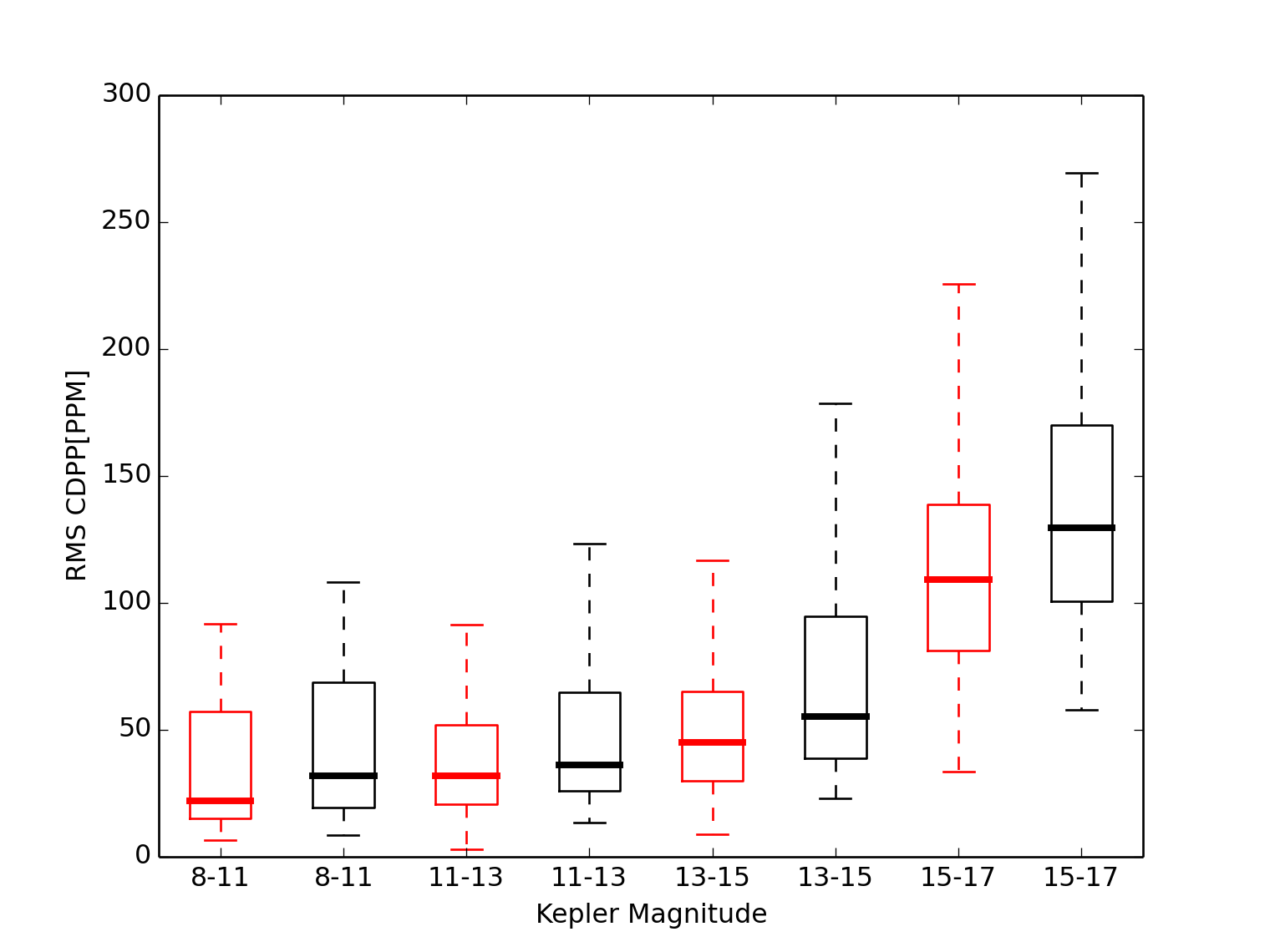
The results illustrate that our approach removes a major part of the variability present in the PDC light curves, while preserving the transit signals. To provide a quantitative comparison, we ran CPM on 1000 stars from the whole Kepler input catalog (500 chosen randomly from the whole list, and 500 random G-type sun-like stars), and estimate the Combined Differential Photometric Precision (CDPP) for CPM and PDC. CDPP is an estimate of the relative precision in a time window, indicating the noise level seen by a transit signal with a given duration. The duration is typically chosen to be 3, 6, or 12 hours (Christiansen et al., 2012). Shorter durations are appropriate for planets close to their host stars, which are the ones that are easier to detect. We use the 12-hours CDPP metric, since the transit duration of an earth-like planet is roughly 10 hours. Fig. 11 presents our CDPP comparison of CPM and PDC, showing that our method outperforms PDC. This is no small feat, since PDC is highly optimized for the task at hand, incorporating substantial astronomical knowledge (e.g., it attempts to remove stellar variability as well as systematic trends).


4 Conclusion
We have assayed half-sibling regression, a simple yet effective method for removing the effect of systematic noise from observations. It utilizes the information contained in a set of other observations affected by the same noise source. The main motivation for the method was its application to exoplanet data processing, which we discussed in some detail, with rather promising results. However, we expect that it will have a large range of applications in other domains as well.
We expect that our method may enable astronomical discoveries at higher sensitivity on the existing Kepler satellite data. Moreover, we anticipate that methods to remove systematic errors will further increase in importance: by May 2013, two of the four reaction wheels used to control the Kepler spacecraft were disfunctional, and in May 2014, NASA announced the K2 mission, using the remaining two wheels in combination with thrusters to control the spacecraft and continue the search for exoplanets in other star fields. Systematic errors in K2 data are significantly larger since the spacecraft has become harder to control. In addition, NASA is planning the launch of another space telescope for 2017. TESS (Transiting Exoplanet Survey Satellite)55 5 http://tess.gsfc.nasa.gov/ will perform an all-sky survey for small (earth-like) planets of nearby stars. To date, no earth-like planets orbiting sun-like stars in the habitable zone have been found. This is likely to change in the years to come, which would be a major scientific discovery.66 6 “Decades, or even centuries after the TESS survey is completed, the new planetary systems it discovers will continue to be studied because they are both nearby and bright. In fact, when starships transporting colonists first depart the solar system, they may well be headed toward a TESS-discovered planet as their new home.” (Haswell, 2010) In particular, while the proposed method treats the problem of removing systematic errors as a preprocessing step, we are also exploring the possibility of jointly modeling systematics and transit events. This incorporates additional knowledge about the events that are looking for in our specific application, and it has already led to promising results (Foreman-Mackey et al., 2015).
Acknowledgments
We thank Stefan Harmeling, James McMurray, Oliver Stegle and Kun Zhang for helpful discussion, and the anonymous reviewers for helpful suggestions and references. C-J S-G was supported by a Google Europe Doctoral Fellowship in Causal Inference.
References
- Christiansen et al. (2012) Christiansen, J. L., Jenkins, J. M., Caldwell, D. A., Burke, C. J., Tenenbaum, P., Seader, S., Thompson, S. E., Barclay, T. S., Clarke, B. D., Li, J., Smith, J. C., Stumpe, M. C., Twicken, J. D., and Van Cleve, J. The Derivation, Properties, and Value of Kepler’s Combined Differential Photometric Precision. Publications of the Astronomical Society of the Pacific, 124:1279–1287, 2012.
- Foreman-Mackey et al. (2015) Foreman-Mackey, D., Montet, B. T., Hogg, D. W., Morton, T. D., Wang, D., and Schölkopf, B. A systematic search for transiting planets in the K2 data. arXiv:1502.04715, 2015.
- Gagnon-Bartsch & Speed (2011) Gagnon-Bartsch, J. A. and Speed, T. P. Biostatistics, 13:539–552, 2011.
- Haswell (2010) Haswell, Carole A. Transiting Exoplanets. Cambridge University Press, 2010.
- Hoyer et al. (2009) Hoyer, P. O., Janzing, D., Mooij, J. M., Peters, J., and Schölkopf, B. Nonlinear causal discovery with additive noise models. In Koller, D., Schuurmans, D., Bengio, Y., and Bottou, L. (eds.), Advances in Neural Information Processing Systems, volume 21, pp. 689–696, 2009.
- Janzing et al. (2009) Janzing, D., Peters, J., Mooij, J., and Schölkopf, B. Identifying confounders using additive noise models. In Bilmes, J and Ng, AY (eds.), 25th Conference on Uncertainty in Artificial Intelligence, pp. 249–257, Corvallis, OR, USA, 2009. AUAI Press.
- Johnson & Li (2007) Johnson, W. E. and Li, C. Adjusting batch effects in microarray expression data using empirical Bayes methods. Biostatistics, 8:118–127, 2007.
- Kang et al. (2008) Kang, H. M., Ye, C., and Eskin, E. Genetics, 180(4):1909––1925, 2008.
- Padmanabhan et al. (2008) Padmanabhan, N., Schlegel, D. J., Finkbeiner, D. P., Barentine, J. C., Blanton, M. R., Brewington, H. J., Gunn, J. E., Harvanek, M., Hogg, D. W., Ivezić, Ž., Johnston, D., Kent, S. M., Kleinman, S. J., Knapp, G. R., Krzesinski, J., Long, D., Neilsen, Jr., E. H., Nitta, A., Loomis, C., Lupton, R. H., Roweis, S., Snedden, S. A., Strauss, M. A., and Tucker, D. L. An Improved Photometric Calibration of the Sloan Digital Sky Survey Imaging Data. The Astrophysical Journal, 674:1217–1233, 2008. doi: 10.1086/524677.
- Pearl (2000) Pearl, J. Causality. Cambridge University Press, 2000.
- Peters et al. (2014) Peters, J., Mooij, J.M., Janzing, D., and Schölkopf, B. Causal discovery with continuous additive noise models. Journal of Machine Learning Research, 15:2009–2053, 2014.
- Price et al. (2006) Price, Alkes L, Patterson, Nick J, Plenge, Robert M, Weinblatt, Michael E, Shadick, Nancy A, and Reich, David. Nature Genetics, 38(8):904–909, 2006.
- Schölkopf et al. (2012) Schölkopf, B., Janzing, D., Peters, J., Sgouritsa, E., Zhang, K., and Mooij, J. M. On causal and anticausal learning. In Langford, J and Pineau, J (eds.), Proceedings of the 29th International Conference on Machine Learning (ICML), pp. 1255–1262, New York, NY, USA, 2012. Omnipress.
- Smith et al. (2012) Smith, J. C., Stumpe, M. C., Van Cleve, J. E., Jenkins, J. M., Barclay, T. S., Fanelli, M. N., Girouard, F. R., Kolodziejczak, J. J., McCauliff, S. D., Morris, R. L., and Twicken, J. D. Kepler Presearch Data Conditioning II - A Bayesian Approach to Systematic Error Correction. Publications of the Astronomical Society of the Pacific, 124:1000–1014, September 2012. doi: 10.1086/667697.
- Spirtes et al. (1993) Spirtes, P., Glymour, C., and Scheines, R. Causation, prediction, and search. Springer-Verlag. (2nd edition MIT Press 2000), 1993.
- Stegle et al. (2008) Stegle, Oliver, Kannan, Anitha, Durbin, Richard, and Winn, John M. Accounting for non-genetic factors improves the power of eQTL studies. In Proc. Research in Computational Molecular Biology, 12th Annual International Conference, RECOMB, pp. 411–422, 2008.
- Stumpe et al. (2012) Stumpe, M. C., Smith, J. C., Van Cleve, J. E., Twicken, J. D., Barclay, T. S., Fanelli, M. N., Girouard, F. R., Jenkins, J. M., Kolodziejczak, J. J., McCauliff, S. D., and Morris, R. L. Kepler Presearch Data Conditioning I - Architecture and Algorithms for Error Correction in Kepler Light Curves. Publications of the Astronomical Society of the Pacific, 124:985–999, 2012.
- Yu et al. (2006) Yu, Jianming, Pressoir, Gael, Briggs, William H, Vroh Bi, Irie, Yamasaki, Masanori, Doebley, John F, McMullen, Michael D, Gaut, Brandon S, Nielsen, Dahlia M, Holland, James B, Kresovich, Stephen, and Buckler, Edward S. A unified mixed-model method for association mapping that accounts for multiple levels of relatedness. Nature Genetics, 38(2):203–208, 2006.