Weak lensing induced by second-order vector mode

We consider the Boltzmann equation for the distribution function, $f(x^{\mu},P^{\mu})$, where we denote the canonical momentum ${\rm d}x^{\mu}/{\rm d}\lambda$ by $P^{\mu}$ and $\lambda$ is the affine parameter. In this subsection we present a brief review of the second-order Boltzmann equation, following [43]. The distribution function for photons obeys the collisional Boltzmann equation since photons interact with electrons via the Compton scattering. The collisional Boltzmann equation for photons is written as

$$\frac{{\rm d}f}{{\rm d}\lambda}(x^{\mu},P^{\mu})=\widetilde{C}[f]~,$$

(6)

where $\widetilde{C}[f]$ is the collision term due to the Compton scattering between photons and electrons in the case of the photon distribution function. For massless neutrinos, the collision term in their Boltzmann equation must vanish. In order to describe the perturbed Boltzmann equation, it is useful to change the coordinate system from the Poisson gauge to the local inertial frame. Hence we use the the momentum in the local inertial frame $p^{\mu}=(E,p\hat{\bm{n}})$ such that $\hat{n}^{i}\hat{n}_{i}=1$ rather than that in the Poisson gauge $P^{\mu}$, hereafter (see [35]). Here $E$ is the energy measured in the local inertial frame, which obeys the Einstein relation $E^{2}-p^{2}=m^{2}$. With these variables, we then expand the photon distribution function up to the second order as

$$f(\eta,\bm{x},p,\hat{\bm{n}})=f^{(0)}(\eta,p)+f^{(1)}(\eta,\bm{x},p,\hat{\bm{n}})+\frac{1}{2}f^{(2)}(\eta,\bm{x},p,\hat{\bm{n}})~.$$

(7)

The zeroth-order distribution function $f^{(0)}(\eta,p)$ is fixed to the Planck distribution. It is convenient to define the brightness function $\Delta^{(1,2)}(\eta,\bm{k},\hat{\bm{n}})$ in Fourier space as

$$\Delta^{(1,2)}(\eta,\bm{k},\hat{\bm{n}})=\frac{\int{dp~p^{3}f^{(1,2)}}(\eta,\bm{k},p,\hat{\bm{n}})}{\int{dp~p^{3}f^{(0)}}(\eta,p)}~,$$

(8)

where we have translated from real space to Fourier space. Furthermore, we expand the brightness function using spherical harmonics to eliminate the angular dependence:

$$\Delta^{(1,2)}(\eta,\bm{k},\hat{\bm{n}})=\sum_{\ell}\sum^{\ell}_{m=-\ell}\Delta^{(1,2)}_{\ell,m}(\eta,\bm{k})(-i)^{\ell}\sqrt{\frac{4\pi}{2\ell+1}}Y_{\ell,m}(\hat{\bm{n}})~.$$

(9)

The brightness function is related to the temperature perturbation of the photons [45]. Here, the multipole coefficient $\Delta_{\ell,m}$ obeys the hierarchical Boltzmann equation

$$\dot{\Delta}^{(1,2)}_{\ell,m}+k\left[\frac{c_{\ell+1,m}}{2\ell+3}\Delta^{(1,2)}_{\ell+1,m}-\frac{c_{\ell,m}}{2\ell-1}\Delta^{(1,2)}_{\ell-1,m}\right]=\mathcal{C}^{(1,2)}_{\ell,m}(\eta,\bm{k})+\mathcal{G}^{(1,2)}_{\ell,m}(\eta,\bm{k})~,$$

(10)

where a dot denotes a derivative with respect to the conformal time, $c_{\ell,m}=\sqrt{\ell^{2}-m^{2}}$, and $\mathcal{C}^{(1,2)}_{\ell,m}$, $\mathcal{G}^{(1,2)}_{\ell,m}$ are the multipole coefficients of the collision and gravitational terms, respectively. The multipole coefficient of the collision term corresponds to the right-hand-side in Eq. (6), whereas the gravitational term comes from the left-hand-side in Eq. (6), i.e., the perturbed geodesic equation for photons. These explicit forms are written in [43]. Although in the first-order perturbations the scalar ($m=0$), vector ($m=\pm 1$), and tensor ($m=\pm 2$) modes are completely decoupled each other, the vector and/or tensor modes can be generated due to the nonlinear interactions of the scalar ones when the second-order perturbations are taken into account. Note that the multipole coefficient of the neutrino distribution function $\mathcal{N}^{(1,2)}_{\ell,m}$ can be formulated in the same manner without the collision term.

We denote this subsection to explicitly write down the evolution equation of the second-order vector mode, which can be derived through the space-space components of the Einstein equation. The second-order Einstein tensor, $G^{i}{}_{j}$ and energy-momentum tensors for the relativistic particles $T_{\rm r}^{i}{}_{j}$ and nonrelativistic particles $T_{\rm m}^{i}{}_{j}$ are given by

	$\displaystyle a^{2}{G^{(2)}}^{i}{}_{j}$	$\displaystyle=$	$\displaystyle 2\Phi^{(1)}\left(\Phi^{(1)}{}^{,i}{}_{,j}-\Psi^{(1)}{}^{,i}{}_{,j}\right)+\Phi^{(1)}{}^{,i}\Phi^{(1)}{}_{,j}-\Psi^{(1)}{}^{,i}\Psi^{(1)}{}_{,j}-\left(\Phi^{(1)}{}^{,i}\Psi^{(1)}{}_{,j}+\Phi^{(1)}{}_{,j}\Psi^{(1)}{}^{,i}\right)$		(11)
			$\displaystyle+\frac{1}{2}\mathcal{H}\left[\dot{h}^{(2)}{}^{i}{}_{j}-\left(\sigma^{(2)}{}^{i}{}_{,j}+\sigma^{(2)}{}_{j}{}^{,i}\right)\right]+\frac{1}{4}\left[\ddot{h}^{(2)}{}^{i}{}_{j}-h^{(2)}{}^{i}{}_{j}{}^{,k}{}_{,k}-\left(\dot{\sigma}^{(2)}{}^{i}{}_{,j}+\dot{\sigma}^{(2)}{}_{j}{}^{,i}\right)\right]$
			$\displaystyle+\left(\Phi^{(2)},\Psi^{(2)}\ \mbox{terms}\right)+\mbox{(diagonal part)}~\delta^{i}{}_{j}~,$

and

	$\displaystyle T_{\rm r}^{(2)}{}^{i}{}_{j}$	$\displaystyle=$	$\displaystyle\rho_{\rm r}^{(0)}\Pi_{\rm r}^{(2)}{}^{i}{}_{j}+\mbox{(diagonal part)}~\delta^{i}{}_{j}~,$		(12)
	$\displaystyle T_{\rm m}^{(2)}{}^{i}{}_{j}$	$\displaystyle=$	$\displaystyle\rho_{\rm m}^{(0)}v_{{\rm m}0}^{(1)i}v_{{\rm m}0j}^{(1)}+\mbox{(diagonal part)}~\delta^{i}{}_{j}~.$		(13)

where $\rho,v,$ and $\Pi$ are the energy density, velocity, and anisotropic stress, respectively. According to the results of the linear perturbations theory, we can split the first-order quantities into the primordial fluctuations $\phi^{(1)}({\bm{k}})$ and the transfer functions as $\Phi^{(1)}(\eta,{\bm{k}})=\phi^{(1)}({\bm{k}})\Phi_{\rm T}(k\eta)$, $\Psi^{(1)}(\eta,{\bm{k}})=\phi^{(1)}({\bm{k}})\Psi_{\rm T}(k\eta)$. The primordial fluctuations in this paper are assumed to be the random Gaussian field characterized by the primordial power spectrum,

$\displaystyle\Braket{{\phi^{(1)}}^{*}({\bm{k}})\phi^{(1)}({\bm{k}}^{\prime})}=(2\pi)^{3}P_{\phi}(k)\delta^{3}_{\rm D}({\bm{k}}-{\bm{k}}^{\prime})~.$

(14)

We will further assume a power-law spectrum in the form

$\displaystyle\frac{k^{3}}{2\pi^{2}}P_{\phi}(k)=\frac{4}{9}\Delta_{\cal R}^{2}(k_{0})\left(\frac{k}{k_{0}}\right)^{n_{\rm s}-1}~,$

(15)

where $k_{0}$ denotes the pivot scale. Hereafter we adopt the scale-invariant spectrum with $\Delta_{\cal R}^{2}(k_{0})=2.4\times 10^{-9}$ [1] and $n_{\rm s}=1$ for simplicity. The velocity perturbations can be related to the scalar metric potentials through

$\displaystyle v_{{\rm m}0i}^{(1)}=-\frac{1}{4\pi Ga^{2}\rho^{(0)}}\partial_{i}\left(\dot{\Phi}^{(1)}+{\cal H}\Psi^{(1)}\right)~.$

(16)

In order to describe the evolution equation for the second-order vector mode, it is convenient to expand the variables in terms of the mode functions. To do this, we adopt spherical coordinate basis vectors which are written in the Cartesian coordinate system as

	$\displaystyle\hat{\bm{n}}$	$\displaystyle=$	$\displaystyle(\sin{\theta}\cos{\varphi},\sin{\theta}\sin{\varphi},\cos{\theta})~,$		(17)
	$\displaystyle{\bm{e}}_{\theta}(\hat{\bm{n}})$	$\displaystyle=$	$\displaystyle(\cos{\theta}\cos{\varphi},\cos{\theta}\sin{\varphi},-\sin{\theta})~,$		(18)
	$\displaystyle{\bm{e}}_{\varphi}(\hat{\bm{n}})$	$\displaystyle=$	$\displaystyle(-\sin{\theta}\sin{\varphi},\sin{\theta}\cos{\varphi},0)~,$		(19)

where we have imposed $\epsilon_{a}^{0}=0$, ${\bm{n}}\cdot{\bm{\epsilon}}_{a}=0$, and ${\bm{e}}_{a}\cdot{\bm{e}}_{b}=\omega_{ab}$ in the observer rest frame. By using these basis vectors, we define the polarization basis as

$${\bm{e}}^{(\pm)}(\hat{\bm{n}})={\bm{e}}_{\theta}(\hat{\bm{n}})\pm\frac{i}{\sin{\theta}}{\bm{e}}_{\varphi}(\hat{\bm{n}})~.$$

(20)

We then introduce the operator $O^{(\pm 1)}_{i}(\hat{\bm{k}})$ which can be defined in terms of the polarization vectors in Fourier space, ${\bm{e}}^{(\pm)}(\hat{\bm{k}})$, as (see, e.g., Refs. [46, 47])

$\displaystyle O^{(\pm 1)}_{i}(\hat{\bm{k}})$

$\displaystyle=$

$\displaystyle\pm\frac{i}{\sqrt{2}}e^{(\pm)}_{i}(\hat{\bm{k}})~,$

(21)

with $\hat{\bm{k}}\equiv{\bm{k}}/k$. Since these operators satisfy the transverse condition, i.e., $\hat{k}^{i}O^{(\pm 1)}_{i}(\hat{\bm{k}})=0$, the vector metric perturbations can be expanded in terms of $O^{(\pm 1)}_{i}$ as

$\displaystyle\sigma_{i}(\eta,\bm{x})$

$\displaystyle=$

$\displaystyle\int{\frac{{\rm d}^{3}k}{(2\pi)^{3}}}\sum_{\lambda=\pm 1}\sigma_{\lambda}(\eta,\bm{k})O^{(\lambda)}_{i}(\hat{\bm{k}})e^{-i\bm{k}\cdot\bm{x}}~.$

(22)

With these conventions, we can obtain the equation of motion for the second-order vector mode by projecting the Einstein equation as

$$\dot{\sigma}^{(2)}_{\lambda}({\bm{k}})+2\mathcal{H}\sigma^{(2)}_{\lambda}({\bm{k}})={\cal S}^{(2)}_{\lambda}({\bm{k}})~,$$

(23)

where ${\cal S}^{(2)}_{\lambda}$ denotes the second-order source terms defined as

	$\displaystyle{\cal S}^{(2)}_{\lambda}({\bm{k}})$	$\displaystyle=$	$\displaystyle\frac{2}{5\sqrt{3}}\frac{1}{k}\left(8\pi Ga^{2}\rho^{(0)}_{\gamma}\Delta^{(2)}_{2,\lambda}(\bm{k})+8\pi Ga^{2}\rho^{(0)}_{\nu}\mathcal{N}^{(2)}_{2,\lambda}(\bm{k})\right)$		(24)
			$\displaystyle+\int\frac{d^{3}k_{1}}{(2\pi)^{3}}4k_{1}\left[\Phi^{(1)}(\bm{k}_{1})\Psi^{(1)}(\bm{k}_{2})\right]\sqrt{\frac{4\pi}{3}}Y^{*}_{1,\lambda}(\hat{\bm{k}}_{1})$
			$\displaystyle-\int\frac{d^{3}k_{1}}{(2\pi)^{3}}\frac{4}{\sqrt{3}}\frac{k^{2}_{1}}{k}\left[\Phi^{(1)}(\bm{k}_{1})\Phi^{(1)}(\bm{k}_{2})+\Psi^{(1)}(\bm{k}_{1})\Psi^{(1)}(\bm{k}_{2})\right]\sqrt{\frac{4\pi}{5}}Y^{*}_{2,\lambda}(\hat{\bm{k}}_{1})$
			$\displaystyle+\sum_{{\rm m}={\rm b},{\rm dm}}8\pi Ga^{2}\rho^{(0)}_{\rm m}\int{\frac{d^{3}k_{1}}{(2\pi)^{3}}}\left[\frac{4}{k}v^{(1)}_{{\rm m}0}(\bm{k}_{1})v^{(1)}_{{\rm m}0}(\bm{k}_{2})\right]\sqrt{\frac{4\pi}{3}}Y^{*}_{1,0}(\hat{\bm{k}}_{1})\sqrt{\frac{4\pi}{3}}Y^{*}_{1,\lambda}(\hat{\bm{k}}_{2})~,$

where $\bm{k}=\bm{k}_{1}+\bm{k}_{2}$, for simplicity, we omit the time dependence in the above equations, and we have translated from the real space to Fourier space. We can see that if we consider the linear theory with perfect fluids, namely, without the right-hand-side in Eq. (24), the vector mode decays with $\propto a^{-2}$. However, in the second-order cosmological perturbation theory, the nonlinear mode coupling between the first-order scalar modes induces a nondecaying vector mode, which is an entirely second-order effect. Consequently, the second-order vector mode imprints on the weak lensing.

Before showing the numerical results of the second-order vector mode, we note the features of our numerical calculation [43, 44]. To solve the second-order Einstein-Boltzmann system Eqs. (10) and (23), we need the first-order perturbations, e.g., $\Phi^{(1)}$ or $\Delta^{(1)}_{\ell,m}$ in the Poisson gauge. We obtain these first-order variables by using the public Boltzmann code such as CAMB [48]. Furthermore, we store the first-order variables in $k$-space from $k_{\rm min}=5.0\times 10^{-5}~[h{\rm Mpc}^{-1}]$ to $k_{\rm max}=5.0\times 10^{2}~[h{\rm Mpc}^{-1}]$. In addition, we solve the Boltzmann hierarchical equation (10) at $\ell=30$ for the first-order Boltzmann equation and at $\ell=25$ for the second-order Boltzmann equation. We checked that the results are stable against these choice.

Before evaluating the effect on the weak gravitational lensing, in this subsection we show the resultant second-order vector mode by performing a fully numerical calculation and we then discuss the feature of the power spectrum under some approximations. To do this, let us define the unequal-time power spectrum for the vector mode as

$$\Braket{\sigma_{\lambda}^{*}(\eta,{\bm{k}})\sigma_{\lambda^{\prime}}(\eta^{\prime},{\bm{k}}^{\prime})}=(2\pi)^{3}\delta_{\lambda\lambda^{\prime}}\delta^{3}_{\rm D}\left({\bm{k}}-{\bm{k}}^{\prime}\right)P_{\sigma}(\eta,\eta^{\prime},k)~,$$

(25)

where $\Braket{\cdots}$ is the ensemble average. We derive an expression for the power spectrum by solving the evolution equation. Equation (23) is easily integrated as

$$\sigma^{(2)}_{\lambda}(\eta,{\bm{k}})=\frac{1}{a^{2}(\eta)}\int^{\eta}_{0}d\eta^{\prime}\left[a^{2}(\eta^{\prime}){\cal S}^{(2)}_{\lambda}(\eta^{\prime},{\bm{k}})\right]~.$$

(26)

Hence we have

$$\Braket{\sigma^{(2)}_{\lambda}(\eta,{\bm{k}}){\sigma^{(2)}_{\lambda^{\prime}}}^{*}(\eta^{\prime},{\bm{k}}^{\prime})}=\frac{1}{a^{2}(\eta)a^{2}(\eta^{\prime})}\int^{\eta}_{0}{\rm d}\eta_{1}\int^{\eta^{\prime}}_{0}{\rm d}\eta_{2}a^{2}(\eta_{1})a^{2}(\eta_{2})\Braket{{\cal S}^{(2)}_{\lambda}(\eta_{1},{\bm{k}}){{\cal S}^{(2)}_{\lambda^{\prime}}}^{*}(\eta_{2},{\bm{k}}^{\prime})}~.$$

(27)

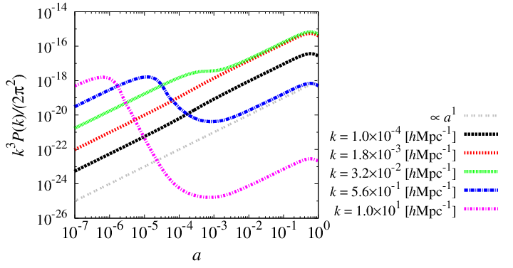
Once we obtain the brightness functions for photons and neutrinos by solving the Boltzmann equation (10) and substitute the first-order results for the scalar metric potentials into Eq. (24), we can obtain the power spectrum for the second-order vector mode though Eq. (27). We now solve the evolution equations for the vector mode by performing a fully numerical calculation. Figure 1 shows the equal-time power spectrum for the vector mode induced by the second-order source terms.

For illustrative purposes to show the dependence on the wavenumber, we adopt the wavenumbers as from $k=10^{-4}~h{\rm Mpc}^{-1}$ to $10^{1}~h{\rm Mpc}^{-1}$. The resultant power spectrum for the second-order vector mode during the radiation-dominated era seems to grow as $\propto a$ on super-horizon scales, while it decays on small scales after it enters the horizon scale. This is because the source of the second-order vector mode, namely the scalar potential, decays during the radiation-dominated era on sub-horizon scales. In contrast, during the matter-dominated era it always evolves as $\propto a(\eta)$ for those wavenumbers. Therefore the second-order vector modes that enter the horizon after the matter-radiation equality time do not undergo the above suppression. In Fig. 2, we plot the dimensionless power spectrum with various values of the redshift. We find that it scales as $k^{1}$ on large scales and $k^{-4}$ on small scales and its peak would be determined by the time of the matter-radiation equality.

We study the analytical description of the power spectrum of the second-order vector mode in the next subsection.

In this subsection, we investigate the feature of the power spectrum for the second-order vector mode analytically. It is difficult to estimate the second-order vector mode analytically including the purely second-order quadrupole moments for photons and neutrinos. However, if we assume that the purely second-order quadrupole moments for photons and neutrinos, $\Delta^{(2)}_{2,\lambda}$ and $\mathcal{N}^{(2)}_{2,\lambda}$, give negligible contributions, the second-order vector metric perturbations are sourced only from the convolution of the first-order scalar metric potentials. Indeed, numerical computations reveal that the corrections of the purely second-order quadrupole moments to the vector mode amount to only about $\lesssim O(10^{-3})\%$ during the matter-dominated era, whereas, the quadrupole moments contribute several tens percent to the vector mode during the radiation-dominated era. Even in the radiation-dominated era, the scalar potentials are still dominant in Eq. (24). In this paper, we focus on the weak lensing signals, which are mainly determined by the contributions after the matter-radiation equality, in which regime the quadrupole moments contribute at most $O(10^{-3})\%$. Therefore, it is sufficient to consider only the scalar metric potentials and we ignore the second-order quadrupole moments, if we give a rough estimation.

To simplify the analysis, we adopt the condition such that the two first-order scalar metric potentials are equal, i.e., $\Phi^{(1)}=\Psi^{(1)}$. While this is valid only if the first-order quadrupole moments are negligibly small, we keep it just for a qualitative understanding of the behavior of the power spectrum for the vector mode. During the radiation-dominated era, the scalar potentials are constant on super-horizon scales while they decay on sub-horizon scales. On the other hand, they freeze on all scales during the matter-dominated era (e.g., see [49]). We note that under this condition the second term of the right-hand-side in Eq. (24) should vanish. This is understood as follows: The condition we impose here implies that ${\bm{k}}_{1}$ and ${\bm{k}}_{2}$ are interchangeable. Moreover, the spherical harmonics has the following property:

$$k_{1}Y^{*}_{1,\lambda}(\hat{\bm{k}}_{1})+k_{2}Y^{*}_{1,\lambda}(\hat{\bm{k}}_{2})=\sqrt{\frac{3}{4\pi}}k\delta_{m,0}~,$$

(28)

where we have imposed ${\bm{k}}={\bm{k}}_{1}+{\bm{k}}_{2}$. As a result, the second line in Eq. (24) gives negligible contributions to the vector mode in the absence of the quadrupole moments.

Let us evaluate the vector mode during the radiation-dominated era. Since the fourth term in Eq. (24) is estimated through Eq. (16) as $8\pi Ga^{2}\rho^{(0)}_{\rm m}v_{{\rm m}0}^{2}\sim(\rho_{\rm m}^{(0)}/\rho^{(0)})\Phi^{2}$, it is suppressed by the factor $\rho_{\rm m}^{(0)}/\rho^{(0)}\ll 1$ compared with the third term. Therefore we found that the third term gives a dominant contribution to the second-order vector mode. Using the explicit expression for the spherical harmonics, the power spectrum for the vector mode induced by the third term in Eq. (24) can be written as

$$\frac{k^{3}}{2\pi^{2}}P_{\sigma}\propto k\int{\rm d}^{3}k_{1}P_{\phi}(k_{1})P_{\phi}(k_{2})T^{2}(\eta,k_{1},k_{2})\left[k^{4}_{1}\sin^{2}{\theta_{1}}\cos^{2}{\theta_{1}}-k^{2}_{1}k^{2}_{2}\sin{\theta_{1}}\sin{\theta_{2}}\cos{\theta_{1}}\cos{\theta_{2}}\right]~,$$

(29)

where ${\bm{k}}_{2}={\bm{k}}-{\bm{k}}_{1}$, $\hat{\bm{k}}\cdot\hat{\bm{k}}_{i}=\cos\theta_{i}$, and the integrated transfer function $T(\eta,k_{1},k_{2})$ is defined in terms of the transfer functions for the scalar potential $\Phi_{\rm T}$ as

$$T(\eta,k_{1},k_{2})=\frac{1}{a^{2}(\eta)}\int_{0}^{\eta}{\rm d}\eta^{\prime}a^{2}(\eta^{\prime})\Phi_{\rm T}(k_{1}\eta^{\prime})\Phi_{\rm T}(k_{2}\eta^{\prime})~.$$

(30)

With a help of the definition of ${\bm{k}}_{2}$ and introducing the direction cosine $\mu_{1}\equiv\cos\theta_{1}$, Eq. (29) can be reduced to

$$\frac{k^{3}}{2\pi^{2}}P_{\sigma}\propto k\int_{0}^{\infty}{\rm d}k_{1}\int_{-1}^{1}{\rm d}\mu_{1}\,k_{1}^{5}P_{\phi}(k_{1})P_{\phi}(k_{2})T^{2}(\eta,k_{1},k_{2})\left(2k_{1}\mu_{1}-k\right)\mu_{1}\left(1-\mu_{1}^{2}\right)~.$$

(31)

To perform this integration analytically, we assume that the transfer function of the scalar potential during the radiation-dominated era is approximated as [49]

$$\Phi_{\rm T}(k\eta)=\frac{1}{1+\left(k\eta\right)^{2}}\quad\left(\eta<\eta_{\rm eq}\right)\,.$$

(32)

Substituting the above transfer function into Eq. (30), we have

$$T(\eta,k_{1},k_{2})=\frac{1}{\eta^{2}k_{1}k_{2}\left(k^{2}_{1}-k^{2}_{2}\right)}\Bigl[k_{1}\arctan\left(k_{2}\eta\right)-k_{2}\arctan\left(k_{1}\eta\right)\Bigr]\quad\left(\eta<\eta_{\rm eq}\right).$$

(33)

In order to evaluate the behavior of the power spectrum, we split the integral of $k_{1}$ in Eq. (31) into two parts: the contributions from $k_{1}>k$ and $k_{1}<k$ for given $k$. In the former case, the dummy variables $\bm{k}_{1}$ and $\bm{k}_{2}$ are related through $k_{2}=k_{1}\bigl[1-(k/k_{1})\mu+O((k/k_{1})^{2})\bigr]$ and the integrated transfer function can be reduced to the following form:

$$T(\eta,k_{1},k_{2})\approx\frac{1}{2k^{3}_{1}\eta^{2}}\left[\arctan(k_{1}\eta)-\frac{k_{1}\eta}{1+(k_{1}\eta)^{2}}\right]\equiv\eta\,\tau_{1}(k_{1}\eta)\quad\left(\eta<\eta_{\rm eq}\right)~.$$

(34)

Hence the contributions from the products of the first-order scalar potentials with their wavelengths shorter than $k$ are

	$\displaystyle\frac{k^{3}}{2\pi^{2}}P_{\sigma}$	$\displaystyle\propto$	$\displaystyle k\int_{k}^{\infty}{{\rm d}k_{1}}\int_{-1}^{1}{{\rm d}\mu_{1}}\,k_{1}^{6}P^{2}_{\phi}(k_{1})\,\eta^{2}\,\left(\tau_{1}(x_{1})\right)^{2}\,\mu_{1}^{2}(1-\mu^{2}_{1})$		(35)
		$\displaystyle\propto$	$\displaystyle k\eta\int^{\infty}_{k\eta}{{\rm d}x_{1}}\left(\tau_{1}(x_{1})\right)^{2}\equiv k\eta\,\beta_{1}(k\eta)~,$

where we have used the scale-invariance of the primordial power spectrum Eq. (15) and we have changed the variable $k_{1}$ to $x_{1}\equiv k_{1}\eta$. Since $\tau_{1}(x)$ behaves as $x^{0}$ for $x\ll 1$ and $x^{-3}$ for $x\gg 1$, the integral of $\beta_{1}$ in Eq. (35) can be evaluated as a function of $k\eta$ : $\beta_{1}\propto(k\eta)^{0}$ for $k\eta\ll 1$, and $\beta_{1}\propto(k\eta)^{-5}$ for $k\eta\gg 1$. Substituting this into Eq. (35), we calculate the contributions from modes with $k_{1}>k$ in Eq. (31):

$\displaystyle\frac{k^{3}}{2\pi^{2}}P_{\sigma}(k<k_{1},\eta<\eta_{\rm eq})\propto\begin{cases}\left(k\eta\right)^{1}&k\eta\ll 1\\ \left(k\eta\right)^{-4}&k\eta\gg 1\end{cases}\,.$

(36)

We can reproduce the behavior of the power spectrum, namely $\propto k^{1}$ for super-horizon scales and $\propto k^{-4}$ for sub-horizon scales, which can be seen in the numerical calculations.

Following the same manner, we can analyze the opposite case, namely $k_{1}<k$. Expanding Eq. (31) in terms of the small quantity $k_{1}/k\ll 1$, we find that the leading order term vanishes due to the angular integration. Furthermore, we also find that the-next leading order term is suppressed by the power $k^{3}_{1}$. Hence the contributions from modes with their wavelengths longer than $k$ are suppressed by the factor $k_{1}/k$ and can be treated as subdominant components. Note that although the above estimations do not work around $k\approx k_{1}$, the results in Eq. (36) is expected to be still correct as long as we estimate the behavior roughly for the following reasons. The integrand in Eq. (31) does not diverge at $k=k_{1}$. The estimations on $k<k_{1}$ and $k>k_{1}$ are smoothly connected. Therefore, the contribution from $k\approx k_{1}$ is at most same order as that from $k<k_{1}$. Combining these results, we conclude that the power spectrum for the second-order vector mode during the radiation-dominated era is determined by the convolution of the scalar potentials with shorter wavelengths.

We discuss the peak shift of the second-order vector mode shown in Fig. 2 from $1+z=10^{5}$ to $10^{4}$. During the radiation-dominated era, the first-order scalar potential remains constant on super-horizon scales while it decays on sub-horizon scales. Therefore, the second-order vector mode can grow due to the constant scalar potential on super-horizon scales. On sub-horizon scales, the second-order vector mode conversely decays due to the decaying scalar potential. As a result, the peak of the second-order vector mode is determined by the horizon scale at the corresponding era and the peak keeps shifting until the matter-radiation equality.

We next consider the vector mode after the radiation-dominated era. The evolution during this era can be easily understood through Eq. (26). Generally, when the second-order source term remains constant (i.e., ${\cal S}^{(2)}_{\lambda}={\rm const.}$), the vector mode evolves as $\sigma^{(2)}_{\lambda}\propto\eta^{1}$. This condition is actually satisfied since the scalar potentials during the matter-dominated era freeze on all scales, as mentioned above. Hence the evolution of the second-order vector mode is given by

$$\frac{k^{3}}{2\pi^{2}}P_{\sigma}\propto\bigl(\sigma^{(2)}_{\lambda}\bigr)^{2}\propto\eta^{2}\propto a^{1}~~~\mbox{(for all scales)}~.$$

(37)

During the matter-dominated era, the shape of the spectrum for the vector mode does not dramatically change since the growing features are the same over all scales. Therefore, the information about the power spectrum during the radiation-dominated era propagates to one during the matter-dominated era, i.e., the dimensionless power spectrum during the matter dominated era is still in proportion to $k^{1}$ for super-horizon scales and $k^{-4}$ for sub-horizon scales, respectively. Although the global feature can be understood as above, in more detail small shifts of the scalar potential such as $\Phi\to 9/10\Phi$ during the matter-radiation equality induce an additional small suppression of the second-order vector mode, as seen in Fig. 1. After the universe is dominated by the dark energy, the scalar potentials begin to decay for all scales, implying that the second-order vector mode generated by these potentials also decays.

Before closing this subsection, we introduce the analytic model of the power spectrum, which is originally derived in [24] (hereafter referred to as MHM). The explicit form of the approximate solution can be written as

$$\frac{k^{3}}{2\pi^{2}}P_{\sigma}^{(\rm MHM)}(k,\eta,\eta^{\prime})=\frac{18}{25^{2}}C_{\rm V}\Delta^{4}_{\mathcal{R}}(k_{0})k^{2}\left(\frac{k}{k_{*}}\right)^{-1}W_{\rm V}(k/k_{*})F(z)F(z^{\prime})~,$$

(38)

where $C_{\rm V}\approx 0.026$, $W_{\rm V}(x)=(1+5x+3x^{2})^{-5/2}$, and $k_{*}=\Omega_{{\rm m}0}h^{2}~{\rm Mpc}^{-1}$ with $\Omega_{{\rm m}0}$ and $h$ being the present cosmological parameter of the nonrelativistic matter and the Hubble constant $H_{0}$ in unit of $100\ [{\rm km\,s^{-1}\,Mpc^{-1}}]$, respectively. The function of a redshift $F(z)$ is given by

$$F(z)=\frac{2g^{2}(z)E(z)f(\Omega_{\rm m}(z))}{\Omega_{{\rm m}0}H_{0}(1+z)^{2}}~,$$

(39)

where $E(z)=\Omega_{{\rm m}0}(1+z)^{3}+\left(1-\Omega_{{\rm m}0}\right)$, $\Omega_{\rm m}(z)=\Omega_{{\rm m}0}(1+z)^{3}/E^{2}(z)$. We adopt $\Omega_{{\rm m}0}=0.27$ as the fiducial value. We denote $f(\Omega_{m}(z))$ and $g(z)$ as the dimensionless linear growth rate and the growth suppression factor, respectively. One can find that $f$ and $g$ are well approximated as $f\approx\Omega_{\rm m}^{7/4}(z)$ and

$$g(z)\propto\Omega_{\rm m}(z)\left[\Omega^{4/7}_{\rm m}(z)-\Omega_{\Lambda}(z)+\left(1+\Omega_{\rm m}(z)/2\right)\left(1+\Omega_{\Lambda}(z)/70\right)\right]^{-1}~,$$

(40)

where $\Omega_{\Lambda}(z)=\left(1-\Omega_{{\rm m}0}\right)/E^{2}(z)$ and we will normalize $g$ so that $g(0)=1$ [50, 51, 24]. We find that the transfer functions derived in MHM and those determined by the numerical calculation match after the matter-radiation equality. However, we should emphasize that for the MHM approximate power spectrum the effect from the evolution of the vector mode over all wave numbers during the radiation-dominated era is assumed to be neglected. As we will see in the subsequent analysis, this approximation leads to the non-negligible difference between the full-numerical and analytic power spectrum.

As we mentioned in the Introduction, the curl mode of the CMB lensing and the B-mode shear can be generated by not the scalar metric perturbations but the vector and/or tensor metric perturbations. In this subsection, to compare with the second-order vector mode, tensor modes are considered as alternative sources of the observables we focus on. In particular, we consider primordial gravitational waves and second-order tensor mode as intriguing examples for tensor metric perturbations. To describe the spectrum for the tensor mode, we define the spin-$\pm 2$ operator $O_{ij}^{(\pm 2)}$ in terms of the polarization vectors as

$\displaystyle O_{ij}^{(\pm 2)}(\hat{\bm{k}})=-\sqrt{\frac{3}{8}}e^{(\pm)}_{i}(\hat{\bm{k}})e^{(\pm)}_{j}(\hat{\bm{k}})\,.$

(41)

Since this operator obviously satisfies the transverse-traceless condition, the second-order tensor metric perturbations can be expanded as

$\displaystyle h_{ij}(\eta,{\bm{x}})=\int\frac{{\rm d}^{3}{\bm{k}}}{(2\pi)^{3}}\sum_{\sigma=\pm 2}h_{\sigma}(\eta,{\bm{k}})O_{ij}^{(\sigma)}(\hat{\bm{k}})e^{-i{\bm{k}}\cdot{\bm{x}}}\,.$

(42)

With these convention, we define the unequal-time power spectrum as

$\displaystyle\Braket{h_{\sigma}^{*}(\eta,{\bm{k}})h_{\sigma^{\prime}}(\eta^{\prime},{\bm{k}}^{\prime})}=\left(2\pi\right)^{3}\delta_{\sigma\sigma^{\prime}}\delta^{3}_{\rm D}\left({\bm{k}}-{\bm{k}}^{\prime}\right)\frac{1}{3}P_{h}(\eta,\eta^{\prime},k)\,.$

(43)

Primordial gravitational waves are generated in the very early Universe and the representative sources for tensor mode. Its effect on the CMB lensing and the shear measurement has been discussed in the literature [21, 20]. For the evolution of primordial gravitational waves, we introduce the PGW transfer function $\mathcal{T}_{h}^{({\rm PGW})}(k\eta)$, which basically describes its sub-horizon evolution. In terms of this, we can write the power spectrum as

$\displaystyle\frac{k^{3}}{2\pi^{2}}P_{h}^{({\rm PGW})}(\eta,\eta^{\prime},k)=r\Delta^{2}_{\mathcal{R}}(k_{0})\left(\frac{k}{k_{0}}\right)^{n_{\rm t}}\mathcal{T}_{h}^{({\rm PGW})}(k\eta)\mathcal{T}_{h}^{({\rm PGW})}(k\eta^{\prime})~.$

(44)

In our analysis we adopt $r=0.1$, $n_{\rm t}=0$ as the fiducial values, and use $\mathcal{T}^{({\rm PGW})}_{h}=3j_{1}(k\eta)/k\eta$ for simplicity. The corrections due to the effects during the radiation-dominated era would be small and we neglect this small correction throughout this paper.

Similar to the case of the vector mode discussed in the previous section, the second-order source terms induce the tensor metric perturbations, which are expected to be one of the possible sources of the curl mode and B-mode shear signals [33]. The analytic model of the power spectrum for the second-order tensor mode induced by the product of the first order scalar metric potentials has been discussed in [24, 49]. The approximate form of the power spectrum derived in [24] is given by

$\displaystyle\frac{k^{3}}{2\pi^{2}}P^{({\rm MHM})}_{h}(\eta,\eta^{\prime},k)=\frac{6}{25}C_{\rm T}\Delta^{4}_{\mathcal{R}}(k_{0})\left(\frac{k}{k_{*}}\right)^{-1}W_{\rm T}(k/k_{*})\mathcal{T}^{({\rm MHM})}_{h}(k\eta)\mathcal{T}^{({\rm MHM})}_{h}(k\eta^{\prime})~,$

(45)

with $C_{\rm T}\approx 0.062$ and $W_{\rm T}(x)=\left(1+7x+5x^{2}\right)^{-3}$. The transfer function for the second-order tensor mode is

$\displaystyle\mathcal{T}^{({\rm MHM})}_{h}(k\eta)$

$\displaystyle=$

$\displaystyle\left(1-\frac{3j_{1}(k\eta)}{k\eta}\right)g^{2}_{\infty}~.$

(46)

The correction factor $g_{\infty}$ attributed to the effect of dark energy is defined as $g_{\infty}\equiv\lim_{z\to\infty}g(z)\approx 1.3136$. We note that this formula is valid only after matter-radiation equality time. While the correction during the radiation-dominated era for the second-order tensor mode has been considered in [49], for the purposes of comparing the second-order vector and tensor modes, we will neglect such correction since it must be small [33].

For comparison, the power spectra for these models at the present time are shown in Fig. 3.

The power spectrum for the second-order vector mode is larger than that for the second-order tensor mode. Therefore, it is expected that the second-order vector mode induces a larger lensing signal than the second-order tensor mode on small scales. Furthermore, on small scales, the second-order vector mode has a larger amplitude than the primordial gravitational waves with $r=0.1$. In other words, the second-order vector mode has the possibility of being detected by cosmological observations on small scales, unlike the primordial gravitational waves. We explain the reason why the discrepancy between the exact vector model and the analytical vector model appears. From Fig. 3, we can see that the amplitude of the exact model is smaller than that of the analytical vector model for $k\gtrsim k_{\rm eq}$, where $k_{\rm eq}\approx 10^{-2}~h{\rm Mpc}^{-1}$ is the horizon scale at the time of matter-radiation equality. For $k\gtrsim k_{\rm eq}$, the analytical vector model does not consider the effect of the small suppression around the matter-radiation equality time. The small suppression on small scales arises because the first order scalar potentials, i.e., the source of the second order vector metric perturbations, decay so rapidly in the radiation dominated era that the source on those scales can sustain the vector perturbations and make them grow proportional to the scale factor only after some time has passed since the matter-radiation equality time (see the blue and magenta lines in Fig. 1). This small suppression is not included in the analytical model. The exact model is about ten times smaller than the analytical vector model for $k\gtrsim k_{\rm eq}$.

From the above discussions, we can understand when the suppression is determined. The analytical vector model does not change its peak since this model is calculated in the flat $\Lambda$CDM model with matters and the cosmological constant. Therefore, the difference between the analytical vector model and exact one is appeared until the matter-radiation equality. In conclusion, the factor about $10$ suppression is determined at the matter-radiation equality time.

The tendency for the second-order vector mode is quite similar to that for the second-order tensor mode in Ref. [33]. In the next section, we will show the numerical results of the weak lensing induced by the second-order vector perturbation.

The projected deflection angle on the celestial sphere in the direction $\hat{\bm{n}}$, $\Delta_{a}(\hat{\bm{n}})$, is generally decomposed into the (parity-even) gradient and (parity-odd) curl modes, expressed as

$$\Delta_{a}(\hat{\bm{n}})=\phi(\hat{\bm{n}})_{:a}+\varpi(\hat{\bm{n}})_{:b}\,\epsilon^{b}{}_{a}~,$$

(47)

where a colon denotes a covariant derivative on the unit sphere and $\epsilon^{b}{}_{a}$ is the covariant two-dimensional Levi-Civita tensor. The quantities $\phi$ and $\varpi$ denote the gradient- and curl-modes of the deflection angle, respectively. Raising or lowering indices of the two-sphere vector are done by $\omega_{ab}$ defined in Eq. (2). In our analysis, we focus only on the curl-mode as the signal of the CMB lensing. We will expand the curl-mode by the spherical harmonics since we observe the scalar and pseudo-scalar lensing potentials on the celestial sphere:

$$\varpi(\hat{\bm{n}})=\sum_{\ell,m}\varpi_{\ell,m}Y_{\ell,m}(\hat{\bm{n}}).$$

(48)

With the coefficients of the harmonics, the angular power spectrum for the curl-mode is defined by

$$C^{\varpi\varpi}_{\ell}=\frac{1}{2\ell+1}\sum_{m=-\ell}^{\ell}\Braket{\varpi^{*}_{\ell,m}\varpi_{\ell,m}}~.$$

(49)

The deflection angle of the light path obeys the null geodesic equation in the perturbed Universe. Solving the spatial parts of geodesic equation for the photon rays at the first-order, we obtain the explicit expression of the curl-mode in terms of the metric perturbations as [23]

$\displaystyle\varpi(\hat{\bm{n}})^{:a}{}_{:a}$

$\displaystyle=$

$\displaystyle-\int^{\chi_{\rm S}}_{0}{\rm d}\chi\frac{\chi_{\rm S}-\chi}{\chi_{\rm S}\chi}\left\{\frac{\rm d}{{\rm d}\chi}\Bigl(\chi\Omega^{a}(\eta_{0}-\chi,\chi\hat{\bm{n}}){}_{:b}\,\epsilon^{b}{}_{a}\Bigr)\right\}~,$

(50)

where $\chi_{\rm S}$ is the comoving distance of the last scattering surface from the observer and $\Omega_{a}$ in the Poisson gauge is written only in terms of the projected vector and tensor modes:

$\displaystyle\Omega_{a}(\eta_{0}-\chi,\chi\hat{\bm{n}})$

$\displaystyle\equiv$

$\displaystyle\Bigl\{-\sigma_{i}(\eta_{0}-\chi,\chi\hat{\bm{n}})+h_{ij}(\eta_{0}-\chi,\chi\hat{\bm{n}})\hat{n}^{j}\Bigr\}\,e^{i}_{a}(\hat{\bm{n}})~.$

(51)

Here we used the Born approximation in Eq. (50) and the basis vectors in real space, $\hat{\bm{n}}$ and ${\bm{e}}_{a}(\hat{\bm{n}})$, have been defined in Eqs. (17)-(19). We can obviously see that the curl-mode is generated by the vector and/or tensor metric perturbations, as already mentioned in the Introduction.

The angular power spectra induced by the vector and tensor modes, respectively, are expressed in terms of the unequal-time power spectra as [23]

	$\displaystyle C^{\varpi\varpi,({\rm v})}_{\ell}=\frac{\pi}{2}\int^{\infty}_{0}k^{2}{\rm d}k\int^{\chi_{\rm S}}_{0}{\rm d}\chi\int^{\chi_{\rm S}}_{0}{\rm d}\chi^{\prime}\,\mathcal{S}^{({\rm v})}_{\varpi,\ell}(k,\chi)\mathcal{S}^{({\rm v})}_{\varpi,\ell}(k,\chi^{\prime})P_{\sigma}(\eta_{0}-\chi,\eta_{0}-\chi^{\prime},k)\,,$		(52)
	$\displaystyle C^{\varpi\varpi,({\rm t})}_{\ell}=\frac{\pi}{2}\int^{\infty}_{0}k^{2}{\rm d}k\int^{\chi_{\rm S}}_{0}{\rm d}\chi\int^{\chi_{\rm S}}_{0}{\rm d}\chi^{\prime}\,\mathcal{S}^{({\rm t})}_{\varpi,\ell}(k,\chi)\mathcal{S}^{({\rm t})}_{\varpi,\ell}(k,\chi^{\prime})P_{h}(\eta_{0}-\chi,\eta_{0}-\chi^{\prime},k)\,,$		(53)

where $S_{\varpi,\ell}^{({\rm v,t})}$ are the weight function for the vector and tensor modes,

	$\displaystyle\mathcal{S}^{({\rm v})}_{\varpi,\ell}(k,\chi)$	$\displaystyle=$	$\displaystyle\sqrt{\frac{(\ell-1)!}{(\ell+1)!}}\frac{j_{\ell}(k\chi)}{\chi}~,$		(54)
	$\displaystyle\mathcal{S}^{({\rm t})}_{\varpi,\ell}(k,\chi)$	$\displaystyle=$	$\displaystyle\frac{1}{2}\frac{(\ell-1)!}{(\ell+1)!}\sqrt{\frac{(\ell+2)!}{(\ell-2)!}}\frac{j_{\ell}(k\chi)}{k\chi^{2}}~,$		(55)

and $P_{\sigma}$ and $P_{h}$ in Eqs. (52) and (53) are the power spectra of the vector and tensor metric perturbations presented in Sec. II, respectively.