Finite size scaling with modified boundary conditions
Abstract
An efficient scheme is introduced for a fast and smooth convergence to the thermodynamic limit with finite size cluster calculations. This is obtained by modifying the energy levels of the non interacting Hamiltonian in a way consistent with the corresponding one particle density of states in the thermodynamic limit. After this modification exact free electron energies are obtained with finite size calculations and for particular fillings that satisfy the so called ”closed shell condition”. In this case the ”sign problem” is particularly mild in the auxiliary field quantum Monte Carlo technique and therefore, with this technique, it is possible to obtain converged energies for the Hubbard model even for . We provide a strong numerical evidence that phase separation occurs in the low doping region and moderate regime of this model.
pacs
71.10.Fd, 71.15.-m, 71.30.+hAfter several years of scientific effort, based on advanced analytical and numerical methods, only very few properties of the 2D Hubbard model have been settled. The 2D Hubbard model is defined in a square lattice containing a finite number () of sites (holes):
| (1) |
with standard notations, the kinetic energy operator being equal to for . In the thermodynamic limit, namely for at given doping fundamental issues such as the existence of a ferromagnetic phase at large ratio and/or the stability of an homogeneous ground state with possible d-wave superconducting properties are still highly debated, as several approximate numerical techniques lead to controversial and often conflicting results. This situation is particularly important right now, since recent progress in the realization of fermionic optical lattices could lead to the experimental realization of the fermionic Hubbard model.
Method: We consider the square lattice and generic finite clusters that satisfy all the symmetries of the infinite system. As well known finite square lattices can be defined by two integers such that , obtained by supercell translation vectors and . In order to fulfill rotation symmetries, two sequences can be defined:
| (2) | |||||
On the other hand translation symmetries are recovered by employing periodic or antiperiodic boundary conditions, the same in both directions and in order to preserve rotation and reflection symmetries.
In the following we would like to consider the most useful sequence of clusters for converging as fast as possible to the thermodynamic limit. A simple technique, well known in strongly correlated lattice models[1] and in realistic calculations[2] is to consider the twisted averaged boundary conditions (TABC) method. This technique allows an exact evaluation of converged thermodynamic quantities (energy, density matrix, etc.) in the non interacting limit.[1] Indeed it has been proven very successful to reduce substantially the finite size effects in several correlated systems.
In the following we follow a different approach analogous to TABC in the requirement to remove finite size effects in the non interacting limit. However the proposed approach can be used more efficiently in combination with the auxiliary field quantum Monte Carlo (AFQMC) method.[3, 4] The latter technique is one of the most powerful ones used so far for the study of the Hubbard model, as it can project out from a mean-field (Slater determinant) state , the exact ground state of the Hamiltonian by the application of the imaginary time propagation , for large . Here we consider variational expectation values (Var) on the state and non variational mixed estimators (no Var) between the previous state and , being the ground state Slater determinant for . Both quantities clearly converge to exact values for large [5].
The sign problem occurs at finite doping and but it is particularly mild when i) the Hamiltonian has a non degenerate ground state, a situation that occurs for particular fillings- the closed shell fillings- in any finite clusters, ii) the auxiliary field transformation is real, as with the proposed approach it is not necessary to sample a complex phase. Until now several reliable and ”numerically exact” calculations have been performed by means of this technique on moderately large clusters (i.e. up to sites and )[6, 7, 8, 9] but it was difficult to establish thermodynamically converged results, especially in the weakly correlated regime. One should also mention that, recently, a remarkable progress has been made, allowing the complete removal of the time discretization error in the propagator[10, 6, 11], a development that will not be used here, as we have preferred to use a small enough time step , such that this systematic error is negligible, at least as far as the ground state energy is concerned.
Let us now introduce the method. Consider a finite cluster. The kinetic energy can be written in Fourier space, by collecting points related by point symmetries to the same energy shell :
| (3) |
where in 2D. We can assume that the energy levels are defined in ascending order. Each shell occurs with some multiplicity and:
| (4) |
where is the number of different energy levels. In the square lattice case we can choose for simplicity clusters that do not contain accidental degeneracies (), namely they are given by the second sequence given in Eq.(2) with PBC (APBC) for odd (even). The fundamental quantity that we are going to use in order to achieve more easily the thermodynamic limit is the density of states :
| (5) |
defined in a way that . This function can be evaluated analytically and/or computed with arbitrary accuracy in the thermodynamic limit for any given lattice model. We partition the energy bandwidth of the lattice (e.g. in the square lattice) in intervals such that:
| (6) |
The above equation define all the levels by simple induction, because once we know , e.g. we can solve the above equation for and we can obtain univocally . Therefore by setting equal to the lowest one electron energy ( in the 2D square lattice), all levels can be computed and their level spacing is in exact correspondence with the density of states. Notice that for the particular symmetry of the DOS in bipartite lattices , due to particle-hole symmetry, it follows that one of the levels is exactly vanishing.
After the above decomposition, in order to fulfill the requirement to have an exact energy for we can modify the energy levels of the kinetic energy in the following way:
| (7) |
where the latter equality comes just from the definition in Eq.(6). In this way the revised kinetic energy is obtained by replacing with in Eq.(3). It is immediate to show that, when we satisfy the closed shell condition, i.e. , within these modified boundary conditions (MBC) we obtain straightforwardly that the ground state energy per site is:
| (8) |
namely the exact energy per site for at the thermodynamic density:
, where the factor two in the above equation takes into account the spin components.
At finite it is quite simple to show that the above sequence of lattices with MBC converges to the exact thermodynamic limit because for large the modification of the levels, as compared to the original ones, becomes irrelevant.
In this way we have several advantages and simplifications:
- •
The Hamiltonian is always real with MBC (a positive property for the sign problem).[12]
- •
The non interacting exact limit is obtained for the closed shell fillings. Thus we expect less size effects just for those particular densities less affected by the sign problem within AFQMC.
- •
The MBC satisfy all the symmetries of the infinite systems. For instance when we apply TABC, each boundary with a non zero twist generally breaks all point spatial group symmetries, maintaining only translation symmetry. This may not affect the average result, but it becomes certainly more difficult to converge to the exact result, i.e. one needs larger projection times in AFQMC due to smaller finite size gaps that occur after a small symmetry breaking perturbation of the Hamiltonian given by a tiny twist of the boundary conditions.
- •
Last but not least, MBC are rather trivial to implement in the AFQMC as it is enough to change the propagator . This matrix is never sparse and has to be computed in advance within AFQMC for its efficient implementation. Thus the use of MBC does not lead to any overhead in the performances of the algorithm.
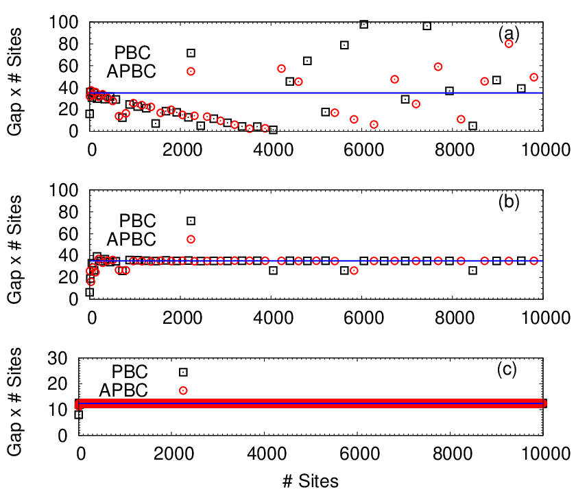


As it is shown in Fig.(1a-c), the most important problem in the usual sequence of finite clusters is that the finite size gap behaves erratically when increases, in spatial dimensionalities and away from commensurate fillings. This precludes to obtain accurate extrapolations to the thermodynamic limit at least for moderate and finite dopings (see e.g. Fig.1d). As it is evident in Fig.(1a-b) the MBC behave much better in this respect. Only few clusters scatter from the converged energy level separations, but they correspond to atypical lattices when at the highest occupied or lowest unoccupied free-electron energy levels. Remarkably a reasonably converged value of this quantity occurs only after few hundreds sites, which is feasible for a numerical approach (see e.g. Fig. 1d).
Results: we have carried out a systematic finite size scaling study of the energy per hole in the moderate regime. As pointed out in the milestone paper by Emery and Kivelson[13] a minimum at doping in the energy per hole, corresponding to a given variational ansatz, implies its instability against phase separation because it is possible to gain energy for by segregating the holes in a hole rich region with the same type of ansatz. In an exact calculation, whenever it is possible to carry out the thermodynamic limit, clearly we have to obtain a constant energy per hole in all the region , just because the compressibility - e.g. the slope in the energy per hole at -, cannot be negative in an exact calculation. As shown in Fig. 2(a), at we can safely reach the thermodynamic limit with the clusters considered, thanks to the very small finite size effects introduced by the method proposed in the previous section, that, in this case, look considerably smaller than standard TABC[8]. The convergence in imaginary time is quite clear also for the most difficult case at small doping (see Fig.2b) and also independent of the initial trial function used. In this case we have used a mean field state with a non zero antiferromagnetic order parameter along the spin direction.[6] In the more difficult cases for larger we have also used a d-wave order parameter in order to converge faster or at least for obtaining the lowest possible variational energies compatible with a reasonable average sign . It is clear that this by no means implies the existence of a non zero superconducting order parameter in the ground state, an issue that will not be discussed in the present work.
At the achieved flat behavior of the energy per hole for clearly indicates the accuracy of the AFQMC at this small coupling, that is indeed able to determine phase separation just by imaginary time projection of an homogeneous trial state. At larger coupling (see Ref.14), though we have not been able to reach the same cluster size and the same length of the projection times, the accuracy in the energy per hole appears acceptable and allow us to determine the phase separated region for (see table). Notice that, in this table, the energy gain to have phase separation can be measured by the difference of the minimum hole energy obtained for the largest clusters at doping and the hole energy extrapolated at using only doping values clearly outside the phase separated region. In other words represents the energy per hole of the uniform phase extrapolated at zero doping. This difference appears to be very large at and less evident for . This is probably the reason why at , there have been several controversial claims[6, 9, 15, 8]. Given this behavior, it is also possible that, at larger , the phase separation may be less evident and may significantly decrease[16], despite some works indicate exactly the opposite effect[17, 8]. It is clear that at large this important issue remains still open. On the other hand, at , we have not obtained evidence of phase separation, because probably we cannot reach enough small doping values with the affordable finite clusters . Indeed at this coupling value also the antiferromagnetic order parameter cannot be detected numerically, being extremely small even at . Since the existence of antiferromagnetism is at the basis of the phase separation argument[13] it is possible that also can be exponentially small at small , as is the case for within the Hartree-Fock theory[3].
| U/t | |||||||||
|---|---|---|---|---|---|---|---|---|---|
| 1 | -0.484(13) | 0.00(1) | -0.49185 | 0.88825 | 1.99156 | -2.46827 | 2.20290 | -0.73928 | 0.00053 |
| 2 | -0.843(1) | 0.067(5) | -0.90164 | 0.73469 | 3.45846 | -4.87765 | 4.03989 | -1.27852 | 0.00062 |
| 3 | -1.125(1) | 0.105(10) | 1.20909 | 0.41515 | 4.84506 | -6.43761 | 4.74676 | -1.35904 | 0.00034 |
| 4 | -1.342(2) | 0.110(15) | -1.35005 | -0.78626 | 9.18032 | -13.03818 | 9.60894 | -2.75519 | 0.0012 |
Conclusions: We have introduced a technique for controlling finite size effects in an efficient way, an approach particularly suited for the AFQMC method. In this way a strong numerical evidence is given that phase separation is robust at small dopings and values. With this approach it is possible to study other possible phases[18, 19, 20], with a better control of finite size effects at incommensurate dopings and weak couplings, as well as it is possible to export the method to other techniques, that may have problem of convergence to the thermodynamic limit especially at weak couplings. Indeed we have preliminary verified that, by choosing boundary conditions that break the symmetry of the lattice (e.g. cylindrical), much better results (i.e. much closer to the thermodynamic limit) can be obtained by correcting the energy levels of the Hamiltonian according to the proposed method. Finally we want to remark that the method can be easily extended to realistic calculations that do not explicitly require a local Hamiltonian[21, 22] as in AFQMC. This can be achieved by considering as an input for the correlated calculation the band-resolved DOS obtained with an uncorrelated Hamiltonian, such as the Khon-Sham one in Density Functional Theory. The same technique as above can be used to reduce finite size effects by preserving charge neutrality even in presence of the Coulomb long range interaction, a property that is difficult to fulfill with TABC, if we require that the non interacting limit should remain exact with a finite supercell calculation.
Acknowledgments I acknowledge useful discussions with F. Becca, S. Yunoki, and L. Tocchio, and support by AICS Riken Kobe and by MIUR COFIN 2010. Part of this research has used computational resources of the K computer provided by the RIKEN Advanced Institute for Computational Science through the HPCI System Research Projects (hp120174 and hp140092) and CINECA ISCRA (grant:HP10C0DZUP).
References
- [1] C. Gros, Phys. Rev. B53, 6865 (1996).
- [2] C. Lin, F. H. Zong and D. M. Ceperley, Phys. Rev. E 64, 016702 (2001).
- [3] J. E. Hirsch Phys. Rev. B31, 4403 (1985).
- [4] S.R. White et al Phys. Rev. B40, 506, (1989); S. Sorella et al. Europhys. Lett. 8, 663 (1989).
- [5] S. Sorella, Y. Otsuka, and S. Yunoki, Sci. Rep. 2, 992 (2012).
- [6] S. Sorella Phys. Rev. B84, 241110 (2011).
- [7] M. Imada, A. Fujimori, Y. Tokura, Rev. Mod. Phys. 70, 1039 (1998).
- [8] Chia-Chen Chang and Shiwei Zhang Phys. Rev. B 78, 165101 (2008); ibidem Phys. Rev. Lett. 104, 116402 (2010).
- [9] E. Khatami, K. Mikelsons, D. Galanakis, A. Macridin, J. Moreno, R. T. Scalettar, and M. Jarrell Phys. Rev. B81, 201101 (2010).
- [10] E. Gull, A. J. Millis, A. I. Lichtenstein, A. N. Rubtsov, M. Troyer and P. Werner, Rev. Mod. Phys. 83, 349 (2011), P. Werner, A. Comanac, L. de’ Medici, M. Troyer, and A J. Millis Phys. Rev. Lett. 97, 076405, (2006); N. V. Prokof’ev and B. V. Svistunov Phys. Rev. B77, 125101 (2008);
- [11] L. Wang, M. Iazzi, P. Corboz and M. Troyer, arXiV:1501.00986v1 (2015); M. Iazzi and M. Troyer, arXiV:1411.0683v1 (2014).
- [12] H. Shi and S. Zhang Phys. Rev. B88, 125132 (2013).
- [13] V. J. Emery, S. A. Kivelson, and H. Q. Lin, Phys. Rev. Lett. 64, 475 (1990).
- [14] See Supplemental Material at [URL] for energy values on several finite size clusters with MBC and .
- [15] F. Becca, M. Capone and S. Sorella Phys. Rev. B62, 12700 (2000)
- [16] L. F. Tocchio, H. Lee, H. O. Jeschke, R. Valenti, and C. Gros Phys. Rev. B 87, 045111 (2013).
- [17] T. Misawa and M. Imada, Phys. Rev. B90, 115137 (2014).
- [18] Y. Deng, E. Kozik,3, N. V. Prokofev, and B. V. Svistunov, arXiV:1408.2088v1 (2014).
- [19] W. Metzner, M. Salmhofer, C. Honerkamp, V. Meden, and K. Schanhammer Rev. Mod. Phys. 84, 299 (2012).
- [20] C. Castellani, C. Di Castro and M. Grilli Phys. Rev. Lett. 75, 4650 (1995).
- [21] G. H. Booth, A. Grüneis, G. Kresse and A. Alavi, Nature 493, 365 (2013).
- [22] S. Zhang, J. Carlson, and J.E. Gubernatis Phys. Rev. Lett. 78, 4486, (1997); J. Carlson ,J. E. Gubernatis, G. Ortiz, and S. Zhang, Phys. Rev. B59, 12788 (1999).