The Mass-Radius Relation of Young Stars, I: UScoCTIO 5, An M4.5 Eclipsing Binary in Upper Scorpius Observed By K2
Abstract
We present the discovery that UScoCTIO 5, a known spectroscopic binary in the Upper Scorpius star-forming region ( days, ), is an eclipsing system with both primary and secondary eclipses apparent in K2 light curves obtained during Campaign 2. We have simultaneously fit the eclipse profiles from the K2 light curves and the existing RV data to demonstrate that UScoCTIO 5 consists of a pair of nearly identical M4.5 stars with , , , and . The radii are broadly consistent with pre-main sequence ages predicted by stellar evolutionary models, but none agree to within the uncertainties. All models predict systematically incorrect masses at the 25–50% level for the HR diagram position of these mid-M dwarfs, suggesting significant modifications to mass-dependent outcomes of star and planet formation. The form of the discrepancy for most model sets is not that they predict luminosities that are too low, but rather that they predict temperatures that are too high, suggesting that the models do not fully encompass the physics of energy transport (via convection and/or missing opacities) and/or a miscalibration of the SpT- scale. The simplest modification to the models (changing to match observations) would yield an older age for this system, in line with the recently proposed older age of Upper Scorpius ( Myr).


I. Introduction
The fundamental properties of stars constitute a bedrock upon which much of astronomy is built, but there remains a paucity of well-characterized stars for calibrating stellar evolutionary models at young ages (1–10 Myr), particularly for low masses (1 ). It is a maxim of stellar astrophysics that the properties and lifecycle of a star are largely set by its mass, and hence it is crucial to calibrate the mass predictions of models. Uncertainties in model-derived properties constitute the dominant systematic error for in-situ measurements of the IMF for young populations [7], determinations of star cluster ages (e.g., Preibisch et al. 70 versus Pecaut et al. 68), comparison of protoplanetary disk properties to those of mature planetary systems [2], and binary formation studies (e.g., Kraus et al. 49, Kraus & Hillenbrand 48, Duchêne & Kraus 30. Mass/age ambiguities strongly limit interpretations for directly-imaged gas giant planets in young populations, where the host-star age and companion luminosity establish the planet mass (e.g., Lafrenière et al. 53 and Ireland et al. 42 versus Pecaut et al. 68, and also Carson et al. 14 versus Hinkley et al. 40).
At present, different model sets predict masses that differ by 50% for nominally solar-mass pre-main-sequence stars at the same point in the - HR diagram (e.g., Hillenbrand & White 39, Torres et al. 91, Gennaro et al. 34, Stassun et al. 85). Furthermore, even the temperature scale for converting spectral type to is uncertain for young stars at the level of 100-200 K (Luhman et al. 56; hereafter L03), constituting a systematic uncertainty on HR diagram positions. Stellar evolutionary models can be tested indirectly, such as by placing binary systems (White et al. 97, Kraus & Hillenbrand 47, Torres et al. 92) or even entire stellar populations [69, 65, 67, 18] on the HR diagram. However, these tests are agnostic to stellar mass and age; they demonstrate whether there are any common ages and masses that reproduce the HR diagram positions, but not whether those values are actually correct. Dynamical masses for young visual binaries have cast much light on this issue (Boden et al. 10, Schaefer et al. 79, Simon et al. 82), and are starting to become available in statistically robust samples Schaefer et al. 78; Rizzuto et al., submitted). However, radius measurements are more time-dependent (particularly among M dwarfs that largely evolve down the Hayashi track to the ZAMS) and have remained elusive. Only a small number of young, low-mass eclipsing binaries are known [94, 63], and with a few well-characterized exceptions [87, 43, 13, 36, 35], those systems are faint and remain only coarsely characterized.
The ages of stars remain similarly uncertain, and are even more difficult to measure without appeals to evolutionary models. Traceback simulations have been notoriously contentious (Ortega et al. 66, Makarov et al. 57, Mamajek & Bell 58), and HR diagram ages can differ significantly depending on the stellar mass range considered and the assumed star formation history [69, 68, 74]. The ongoing debate over the age of the Upper Scorpius OB association and other young populations [65, 8, 58] demonstrates that systematic errors remain at the level of factors of 2. However, if an evolutionary model reproduces all of the other observable parameters of a star (mass, radius, , and ), then the model-derived age could represent the most robust possible theoretical estimate of the age for that stellar population.
To address these fundamental issues of stellar astrophysics, and to look for planets, we have initiated a search for eclipsing/transiting systems among all of the known and suspected members of Upper Scorpius and Ophiuchus that fell in the footprint observed by K2, the extended Kepler mission [41] during its Campaign 2. These observations comprised 79 continuous days of observing with a 30 minute cadence, with no gaps, and hence are ideal for identifying all eclipsing binaries with periods on the order of this duration or shorter. In total, we proposed observations of 657 confirmed members (GO2052, PI Covey) and 759 likely candidate members (GO2063, PI Kraus) that were optically visible ( mag). Given the size of our sample and the known frequency of short-period binary systems in the field [71], we expect that 10–15 new eclipsing binaries should be discovered.
The young Upper Scorpius member UScoCTIO 5 (Figure 1)11 1 The USco candidates identified by Ardila et al. [3] are sometimes abbreviated as “USco NN”. However, SIMBAD has assigned the name “USco 5” to different candidate member by Sciortino et al. [80]. We caution the reader to not confuse the two sources if pursuing additional followup observations. was a high-priority target in our program since it is a known spectroscopic binary, first reported and characterized as such by Reiners et al. [73]. The membership of UScoCTIO 5 in Upper Scorpius was first proposed by Ardila et al. [3], based on its HR diagram position, line of sight extinction, and the presence of H emission; this membership was confirmed by Reiners et al. [73] based on the presence of lithium absorption that constrains the age to be Myr. Reiners et al. [73] also detected the presence of two sets of spectral lines in their first high-resolution spectrum, and subsequently obtained enough additional spectroscopic observations to determine the period ( days), the orbital elements, and a minimum mass (modulo the sine of the orbital inclination). Their inferred minimum mass ( ) was larger than the mass predicted by evolutionary models, which suggested both that the models could require modifications or additional physics, and that the system could be close to edge-on (and hence could show eclipses).
In this paper, we report that UScoCTIO 5 is indeed oriented to show both primary and secondary eclipses in its K2 light curve. We re-interpret the sum of data available for the system to determine masses and radii for each star, to test different evolutionary model tracks against the empirical constraints of this system, to calculate an empirical constraint on the SpT- conversion for young mid-M stars, and to determine a new semi-empirical age estimate for the Upper Scorpius OB association.
II. K2 Light Curves


II.1. K2 Photometry
We downloaded the target pixel files (TPFs) for UScoCTIO 5 from the Mikulski Archive for Space Telescopes (MAST), where it is stored under its Ecliptic Plane Input Catalog (EPIC) identification number 205030103. This data consists of 3811 1012 pixel stamp images centered on UScoCTIO 5, acquired between 2014 August 23 and 10 November.
Telescope pointing for K2 is unstable, due to the failure of a second reaction wheel during the Kepler prime mission in May of 2013. As a result, the centroid of UScoCTIO 5 drifts at a rate of 0.1″, or 0.02 pixels, per hour. While this movement is relatively small, associated detector sensitivity variations at the few percent per pixel level compromise the otherwise exquisite photometry. To compensate for these effects, onboard software checks the pointing every six hours and initiates a thruster firing if the roll angle has exceeded a threshold. The result is jumps in position (and hence measured flux) on this timescale.
To minimize the effect of jumps on the photometry, we determined the stellar centroid position independently for each pixel stamp. TPF headers provide a rough world coordinate system solution which is the same for all images, but these are not precise enough to center the target. We therefore cut out a 77 pixel substamp around the nominal target position (i.e., the green dot in the left side of Figure 1), and determined a flux-weighted centroid from these pixels. The drift in these centroids over time can be seen in the bottom panels of Figure 2.
We then placed photometric apertures at each centroid location, extracting photometry with a set of circular apertures from 1.0 to 4.0 pixels in radius, at intervals of 0.5 pixels, and subtracting the background as determined from a wider annulus. The circular aperture is assumed to have a boundary that intersects the square pixels along an arc, with fractional flux per pixel integrated geometrically for pixels neither fully inside nor outside the circular aperture. We found that photometric noise levels after detrending for position jump effects (see Section 2.2) were minimized with the 1.5-pixel aperture. This size has the additional advantage of being small enough so as to avoid flux contamination from other stars lying 10″ away. The chosen aperture is shown as a red circle in Figure 1.
To remove errant data, we discarded the first 93 light curve points, for which the pixel positions were particularly different compared to the rest of the time series. We also removed points with detector anomaly flags. Finally, we pruned points lying more than five standard deviations off the median light curve trend (excluding points within or around eclipses). The resulting raw light curve is displayed in Figure 2.
II.2. Detrending of Instrumental Effects and Stellar Variability
Before eclipse fitting was performed, the K2 light curve of UScoCTIO 5 was corrected for instrumental artifacts and detrended to remove starspot signatures that dominate UScoCTIO 5’s out-of-eclipse light curve. The degradation of Kepler’s pointing control in the K2 mission results in light curves which, in many cases, are dominated by the target star’s path across small (1-2%) sensitivity variations in Kepler’s detector. However, as Vanderburg & Johnson [95] and Vanderburg et al. [96] have shown, the well-behaved nature of this correlation allows the removal of much of this signature by applying a position-dependent correction to each K2 light curve.
We applied such a correction to UScoCTIO 5’s light curve, removing the systematic structure associated with the drift of the K2 focal plane. To infer the correlation between UScoCTIO 5’s xy position on the detector and the sensitivity of the K2 light curve, we first performed an initial detrending of UScoCTIO 5’s light curve to remove the intrinsic stellar variations that is ubiquitous to young stars (e.g., Cody & Hillenbrand 21, Cody et al. 22, Cody et al. 23) and whose amplitude is 10x larger than the systematic pointing artifacts. We removed these stellar variations using the SuperSmoother algorithm, originally developed by Friedman (1984) and subsequently implemented in python by Vanderplas (2015; 10.5281/zenodo.14475), by dividing the raw light curve by an alpha=0 supersmoothed fit. The alpha parameter provides a mechanism for biasing the SuperSmoother fit against high frequency components (i.e., providing ’bass enhancement’ in Friedman’s original treatment); an alpha=0 fit corresponds to an unbiased fit, which preserves the ability to fit and correct for high frequency stellar variations in the target light curve.
With the large-scale stellar variability signatures removed, the systematic structure due to K2’s pointing drift dominated the normalized light curve; we removed this structure by dividing the flux in each epoch of UScoCTIO 5’s raw light curve by the median normalized flux of the 10 data points in the normalized light curve whose xy positions are closest to that of the epoch in question. The correlation between K2’s sensitivity and UScoCTIO 5’s xy position underwent a clear change halfway through campaign 2, when the direction of the torque resulting from the incident solar flux changed to the opposite direction. As a result, we corrected the portions of the light curve taken before and after epoch 2102 independently.22 2 In the text and in Figures 2 and 3, we use the Kepler time coordinate system for the K2 light curve where epoch = BJD - 2454833.
Finally, having applied this pointing correction to USco CTIO 5’s raw light curve, we then again used an 0 SuperSmoother fit to detrend the light curve and remove the large-scale starspot signatures prior to fitting the eclipse profiles. The remaining light curve still showed long-term variations at the level of 3 millimagnitudes, so we removed this remaining small signal by fitting (using datapoints outside eclipse) and subtracting a DC offset for 12 hours around each eclipse. We show the raw, instrumental-detrended, and instrumental/stellar-detrended light curves in Figure 3.
III. High-Resolution Spectroscopy and Radial Velocities
| Epoch | Epoch | Wavelength | ) | SNRaaMeasurements of the spectrum’s SNR and the components’ flux ratio are made at Å if that wavelength is included in the observation, and at Å otherwise. | bbWe report and as the standard deviation of the Gaussian fits to the two stars’ broadening functions, which is a measure of both the instrumental broadening and the rotational broadening. | bbWe report and as the standard deviation of the Gaussian fits to the two stars’ broadening functions, which is a measure of both the instrumental broadening and the rotational broadening. | |||
|---|---|---|---|---|---|---|---|---|---|
| (UT Date) | (HJD-2450000) | Range (Å) | (sec) | (km/s) | (km/s) | (km/s) | (km/s) | ||
| 20030611 | 2801.94316 | 6400-8700 | 900 | 49 | -36.78 0.18 | 8.05 0.10 | 33.22 0.17 | 8.09 0.27 | 0.915 0.034 |
| 20040509 | 3134.96680 | 7000-9250 | 900 | 50 | -9.18 0.12 | 6.65 0.32 | 4.29 0.13 | 7.18 0.24 | 1.045 0.052 |
| 20040510 | 3136.00935 | 7000-9250 | 1200 | 52 | -15.49 0.09 | 6.92 0.22 | 11.47 0.21 | 7.01 0.27 | 0.941 0.011 |
| 20040511 | 3136.90724 | 6400-8700 | 1200 | 43 | -22.05 0.16 | 7.71 0.23 | 17.25 0.19 | 7.27 0.28 | 0.908 0.026 |
| 20040511 | 3137.00804 | 6440-8750 | 900 | 39 | -22.53 0.10 | 7.80 0.14 | 18.27 0.11 | 7.66 0.14 | 0.932 0.020 |
| 20040511 | 3137.13712 | 6440-8750 | 400 | 5 | -24.44 0.17 | 7.74 0.21 | 18.57 0.16 | 7.52 0.31 | 0.951 0.044 |
| 20040513 | 3139.13254 | 4480-6890 | 400 | 17 | -35.89 0.20 | 7.59 0.21 | 31.65 0.20 | 8.04 0.19 | 0.932 0.034 |
| 20050302 | 3432.06727 | 5720-8570 | 900 | 33 | 17.79 0.13 | 7.85 0.13 | -24.12 0.11 | 7.87 0.12 | 0.922 0.017 |
| Gl 83.1 | 5741.13595 | 4320-8750 | 120 | 46 | .. | .. | .. | .. | .. |
| Gl 83.1 | 5930.69346 | 4320-8750 | 120 | 71 | .. | .. | .. | .. | .. |
| Gl 447 | 5933.16968 | 4320-8750 | 120 | 130 | .. | .. | .. | .. | .. |
| HZ 44 | 5931.18067 | 4320-8750 | 120 | 43 | .. | .. | .. | .. | .. |
| Epoch | HJD | |||
|---|---|---|---|---|
| (UT Date) | (days) | (Å) | (Å) | (Å) |
| 20030611 | 2801.94316 | -6.1 | 0.32 | 0.23 |
| 20040511 | 3136.90724 | -4.8 | 0.29 | 0.27 |
| 20040511 | 3137.00804 | -3.8 | 0.31 | 0.29 |
| 20040511 | 3137.13712 | -4.0 | 0.25 | 0.20 |
| 20040513 | 3139.13254 | -4.7 | 0.32 | 0.27 |
| 20050302 | 3432.06727 | -4.6 | 0.34 | 0.30 |
High-resolution spectroscopic measurements for UScoCTIO 5 were already reported by Reiners et al. [73], who obtained 22 epochs in 2003–2005 with the optical echelle spectrographs Keck-I/HIRES, Magellan/MIKE, and Blanco/Echelle. They extracted the difference between the primary and secondary star RVs () for the system in each epoch, determined from a cross-correlation with the dwarf standard star Gl 406. They reported a best-fit orbit with days, , , AU, deg, and days (MJD). However, since the K2 light curve offers precise constraints on the period and a combination of the eccentricity and longitude of periastron, we have refit the orbit as part of our analysis.
We have adopted the Magellan and Blanco measurements directly from the analysis by Reiners et al. [73]. Based on the RMS scatter that they reported for their measurements around the best-fit orbit, the typical uncertainty in each measurement is m/s. For the Keck-I/HIRES data, we have downloaded the observations from the Keck archive and reanalyzed the spectra to measure absolute RVs for each component. These absolute velocities are needed in order to measure the mass ratio of the system, and hence the masses of the individual component stars.
Our analysis of the HIRES data is very similar to the methods described in Kraus et al. [51] and Kraus et al. [50]. We extracted and wavelength-calibrated each spectrum using the MAKEE pipeline33 3 http://spider.ipac.caltech.edu/staff/tab/makee, refining the wavelength solution by cross-correlating the 6800Å or (preferably) 7600Å telluric absorption bands against those of the spectrophotometric standard star HZ 44 [62]. For each spectrum of UScoCTIO 5, we then measured the broadening function (Rucinski 1999)44 4 http://www.astro.utoronto.ca/~{}rucinski/SVDcookbook.html with respect to our own Keck/HIRES observations of two standard-stars over a total of three epochs: one observation of Gl 447, and two separate observations of Gl 83.1. Both standard stars have temperature and metallicity similar to UScoCTIO 5 (SpT=M4–M5 and ; Rojas-Ayala et al. 76, Mann et al. 2015b). The broadening function is a better representation of the rotational broadening convolution than a cross-correlation, since it is less subject to “peak pulling” and produces a flatter continuum. We fit each broadening function with two Gaussian functions to determine the absolute primary and secondary star RVs ( and ), the standard deviations of the lines due to rotation and instrumental resolution ( and ), and the average flux ratio across all well-fit orders (which is estimated from the ratio of areas for the two peaks of the broadening function).
We list these measurements in Table 1. For those spectra that include the 6500-6700Å region, we also report equivalent widths of H emission (which was never fully resolved due to the intrinsic thermal broadening of the chromosphere, and hence we report as a single value) and Li6708 absorption (which was resolved in all epochs) in Table 2. The equivalent widths are measured with respect to the continuum of the full composite spectrum, but individual stellar values can be determined from the flux ratio of the spectra (which is nearly constant across the entire wavelength range of these spectra). We also show narrow wavelength ranges around H and Li6708 in each spectrum in Figure 4.
IV. Spectral Classification, Extinction, Temperature, and Luminosity


| Filter | (mag) | Reference |
|---|---|---|
| 17.806 0.203 | APASS [37] | |
| 16.192 0.010 | APASS [37] | |
| 16.975 0.074 | APASS [37] | |
| 15.482 0.042 | APASS [37] | |
| 15.385 0.050 | CMC15 [31] | |
| 13.708 0.011 | APASS [37] | |
| 11.172 0.023 | 2MASS [26] | |
| 10.445 0.026 | 2MASS [26] | |
| 10.170 0.021 | 2MASS [26] | |
| 10.036 0.023 | ALLWISE [25] | |
| 9.838 0.020 | ALLWISE [25] | |
| 9.648 0.047 | ALLWISE [25] |

IV.1. Intermediate-Resolution Spectroscopy
To better determine its spectral type and extinction, we observed UScoCTIO 5 on 2015 April 1 using the Wide-Field Spectrograph (WIFES) on the ANU 2.3m telescope. These observations are identical to those described by Rizzuto et al. [74], which describes the data and procedures in more detail. WIFES is an integral field spectrograph with an FOV of 3825″, feeding red and blue arms. We configured the red arm to deliver a spectral resolution of across a wavelength range of 5300–7000Å; the flux to the blue arm was not sufficient to deliver useful data. We observed UScoCTIO 5 with an integration time of s, yielding at 6600Å. We processed the raw WIFES data with the “WiFeS PyPeline” [19] software in order to extract a spectral data cube. We then measured the flux in each spectral channel using PSF-fitting photometry with a Moffat profile, integrating the profile to measure the total flux from the science target in each channel and subtracting the sky background implied from the DC offset of the PSF fit. We show the extracted spectrum in Figure 5 (left); for further detail regarding the extraction process see Rizzuto et al. [74].
IV.2. Archival Photometry
The geometric determination of radii offers the intriguing possibility of directly measuring empirical temperatures, as long as an accurate luminosity can be determined. While it is possible to estimate the stellar luminosity from a single flux and a corresponding bolometric correction, it should be more accurate to compile a broadband SED and add up the flux. This strategy also minimizes model-dependent uncertainties in the assumed bolometric correction. To that end, we also have compiled all of the available (component unresolved) photometry in all-sky surveys. As we summarize in Table 3, we have used photometry from 2MASS (,,; Cutri et al. 26), AllWISE (, , ; Cutri & et al. 25), CMC15 (; Evans et al. 31), and APASS (, , , , ; Henden et al. 37).
IV.3. Atmospheric Properties
We have used the low-resolution optical spectrum from WIFES (Section 4.1; Figure 5, left) to calculate a joint constraint on the spectral type and extinction of the UScoCTIO 5 system. We compared the observed spectrum to a sequence of field M dwarfs compiled from SDSS [9], that we artificially reddened using an reddening law [77]; the best spectrum is an M4.5 dwarf that has been reddened by mag. In Figure 5 (right), we show the best-fitting value as a function of spectral type for the full grid of standards, as well as contours in the surface. It is not straightforward to convert these contours to a statistically robust confidence interval because spectra show strong covariances across wide wavelength ranges due to both astrophysical and instrumental errors. However, the interval of denotes the range across which the residuals become visually apparent, and hence represent an upper limit on the uncertainty in the spectral classification. Since spectral types themselves are only defined by half-subclasses, then we assess a final uncertainty of 0.5 subclass on the spectral type and a corresponding uncertainty of mag on the extinction.
The conversion from spectral type to temperature has been a matter of longstanding debate in the star formation community. It is well known that this conversion is gravity-sensitive for M dwarfs (e.g., Luhman 55) and perhaps even for earlier-type stars [67], such that giants of equivalent spectral type are several hundred degrees hotter than dwarfs. L03 proposed an “intermediate gravity” temperature scale that might be appropriate for young stars, constructed from an interpolation of the dwarf and giant scales that makes the GG Tau system look coeval (as per White et al. 97). Given the spectral type of M4.50.5, the inferred temperature on this intermediate-gravity scale is K. The dwarf scales would imply a lower temperature of K according to Leggett et al. [54], or warmer temperatures of K from more recent scales (Rajpurohit et al. 72; Mann et al. 2015b) while the giant scale [93] would imply a higher temperature of K. Herczeg & Hillenbrand [38] more fully review the wide range of other proposed temperature scales, which yield temperature estimates spanning 3080–3305 K for an M4.5 dwarf star; they develop an independent young star temperature scale that would predict K for UScoCTIO 5. For this work, we adopt the temperature scale of L03 and the corresponding spectroscopic temperature of K in order to remain consistent with the previous literature, but we also remind the reader that substantial systematic uncertainties remain.
As we discuss further in Section 6.2, it is possible to empirically anchor the SpT- relation at M4.5 using our geometric radius measurements if we can also measure the luminosity. To that end, we computed following the procedure from Mann et al. (2015b). We used a set of solar-metallicity, BT-SETTL models [1] built with the Caffau et al. [12] solar abundances, which better reproduce the observed spectra of field M dwarfs than BT-SETTL models utilizing the Asplund et al. [4] abundances [60]. We selected grid points spanning the range of temperatures found above, each of which we reddened by a grid of extinction values consistent with the value and error derived using the empirical spectrum. We then scaled each model spectrum to give the best agreement (lowest ) between synthetic and observed photometry and integrate over the (un-reddened but scaled) model spectra to determine . The range of temperatures and extinction values produced a range of values, which we use as an estimate of the uncertainty. The best fit model ( K, mag) is shown in Figure 6. To convert from to , we assume a distance of pc, consistent with the mean and scatter seen for BAF stars in Upper Scorpius (e.g., de Zeeuw et al. 27, Rizzuto et al. 75). The 20% uncertainty in extinction dominates the uncertainty in (5%). The 10% uncertainty in the distance, which propagates to a 20% uncertainty in the luminosity, represents the dominant source of uncertainty in . Using the model to fill the gaps between the photometry, we find a total bolometric flux of erg/s/cm2. For an assumed distance of pc, the corresponding luminosity is , or individual component luminosities of .
V. Results
| Orbital Parameters | |
|---|---|
| (HJD) | 56914.490 0.026 |
| (days) | 34.00073 0.00007 |
| (AU) | 0.17749 0.00031 |
| 0.26741 0.00011 | |
| (deg) | 87.912 0.010 |
| (deg) | 355.13 0.30 |
| (km/s) | -2.64 0.07 |
| Stellar Bulk Parameters | |
| () | 0.6452 0.0034 |
| 0.963 0.007 | |
| () | 0.3287 0.0024 |
| () | 0.3165 0.0016 |
| () | 1.644 0.008 |
| 0.972 0.011 | |
| () | 0.834 0.006 |
| () | 0.810 0.006 |
| (cm/s2) | 4.11 0.01 |
| (cm/s2) | 4.12 0.01 |
| Stellar Atmospheric Parameters | |
| 0.999 0.017 | |
| 1.000 0.004 | |
| (mag) | 1.06 |
| SpT | M4.5 0.5 |
| (K) | 3200 75 |
| (K) | 3085 105 |
| (erg/s/cm2) | |
| Parameters Using Distance | |
| () | |
| () | |
| (K) | |
| (K) | |
| Infrared Flux Method Distance | |
| (pc) | 144.4 6.6 |
| (pc) | 135.1 8.8 |
V.1. Fitting for Orbital and Stellar Parameters
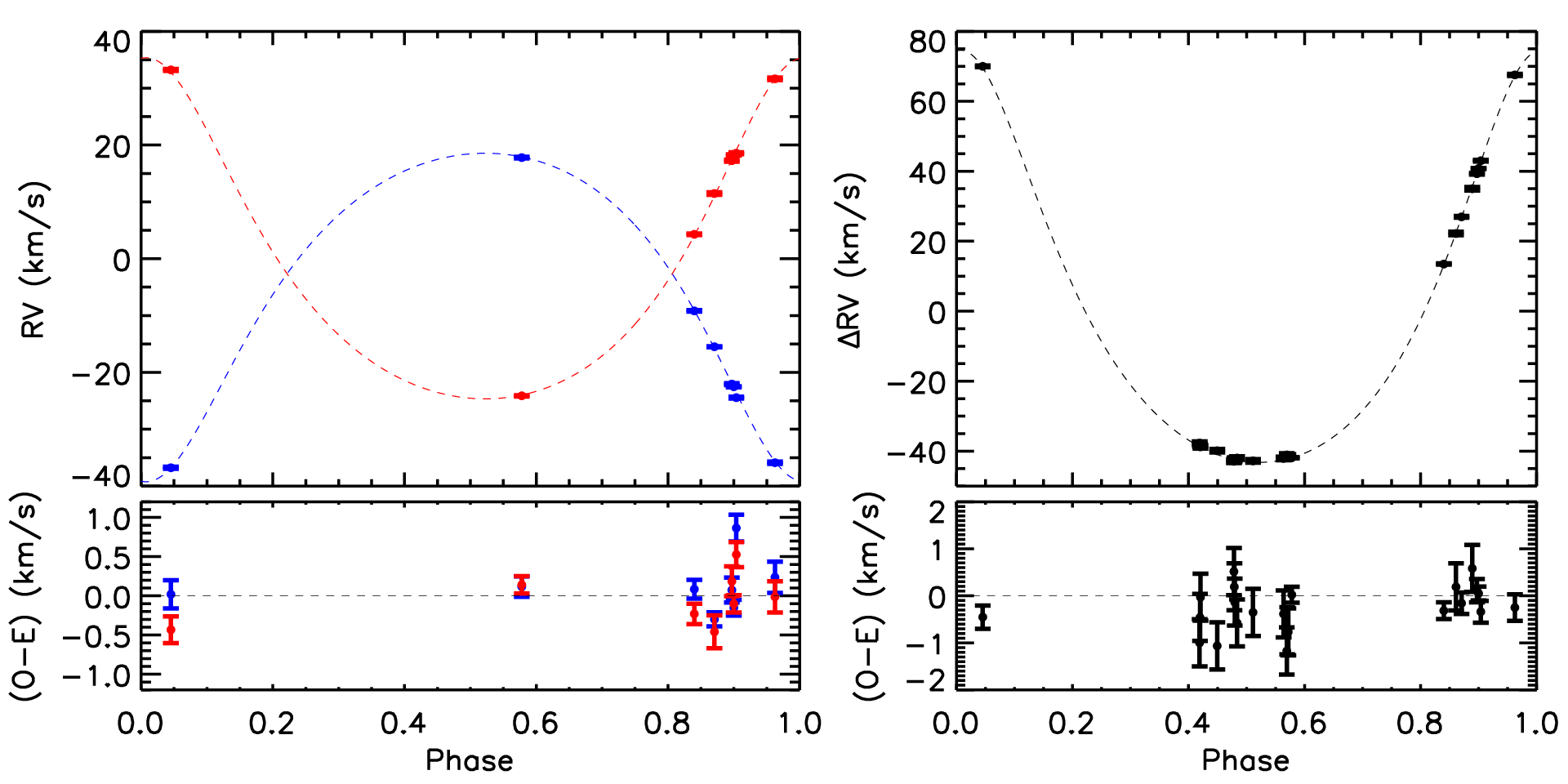
In the simple case of a tidally circularized orbit, fitting for the parameters of an eclipsing binary is a straightforward and separable problem: the component masses (moduli ) can be derived from the radial velocity curve, while the inclination, period, radii, and stellar flux ratio can be derived from the light curve. However, eccentric systems are more complicated, with many covariances between parameters. For example, while the RV curve provides a direct measurement on the eccentricity and the argument of periapse , the orbital phases of primary and secondary eclipse can provide a very tight joint constraint on both parameters. The durations of the eclipses provide a further constraint on and , as well as posing a joint constraint on the inclination and surface brightness ratio (since the surface areas occulted can differ between the primary and secondary eclipses). Finally, since the RVs and photometry were measured nearly a decade apart, then timekeeping errors could lead to covariances in the parameters. For a system this wide, apsidal motion should be negligible on decade timescales (e.g., Feiden & Dotter 32), so we do not expect the orbital parameters to have changed between the epochs of the RV data and K2 data.
To properly account for these covariances, we have constructed a Markov-Chain Monte Carlo (MCMC) procedure to simultaneously fit both the RV curve and the light curve using a full model of all parameters. We specifically consider a model where the explicitly fit parameters are 6 orbital elements (, , , , , and , neglecting in the absence of spatially resolved information), the mass ratio of the system , the systemic radial velocity , the sum of the stellar radii , the ratio of the stellar radii , and the ratio of stellar fluxes through the Kepler bandpass .
We note that the convention for eclipsing binaries is not to fit for , but rather for a temperature ratio or temperature difference (indeed, as we have done in the past; Kraus et al. 51). In principle, the ratio of surface brightnesses can be described by the ratio of temperatures; in the limiting case of a pure blackbody, the relation is exact and analytic. However, cool stellar atmospheres are notably non-blackbody, making this relation more complex. Traditional fitting codes like the Wilson-Devinney algorithm (Wilson & Devinney 98, and extensive updates thereof) parametrize this relation using Kurucz model atmospheres [52]. However, those codes typically only extend to K (hotter than our observed targets), and the conversion from temperature ratio to flux ratio is not easily quantified or changed. We find it more straightforward to fit directly for the flux ratio in the Kepler bandpass, and then deal with the conversion to a temperature ratio explicitly. This choice can also be found in other fitting codes such as JKTEBOP [84], which shares many design choices with our procedures.
In executing our MCMC procedure, we use analytic equations to construct a predicted RV curve against which we can compare the observations and measure the residuals. In order to isolate potentially correlated uncertainties between the measurements of the primary and secondary star at each epoch (such as from uncertainties in the wavelength scale), we chose to fit the primary star RV (for the 8 epochs of HIRES data) and the difference in RV (for all 22 epochs). Some fit parameters (such as the semimajor axis, and hence the total system mass) only depend on , while others (such as the system velocity and the mass ratio) necessarily depend on the individual component RVs, so this choice ensures that the correlated RV errors between primary and secondary star will not unnecessarily inflate the uncertainty in parameters that do not require component-resolved measurements.
The analysis of the light curve is less straightforward. As we mention above, the Wilson-Devinney code is the gold standard of the field due to the wide range of physical effects (such as reflected light and tidal distortion) that it can reproduce. However, most of these physical effects are not needed for a binary with a semimajor axis of nearly 0.2 AU, and the architecture needed to encompass them results in a long runtime (of order seconds) to produce a single model. Furthermore, the Wilson-Devinney solution for stars that fall outside their modeled temperature range (interpolation between the coolest model and a blackbody) is also not appropriate for cool stars, meaning that its implicit conversion from to a temperature ratio would not be correct.
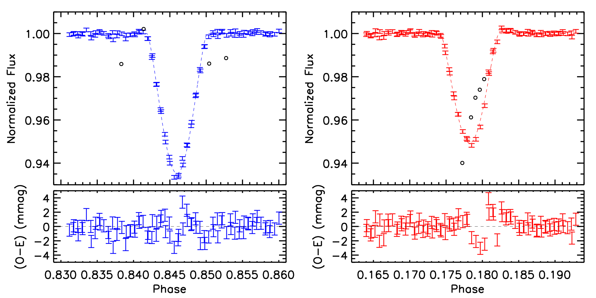
We therefore have instead constructed an analytic formalism that uses the work of Mandel & Agol [59] to calculate the total light removed from the system due to occultation of whichever star is more distant. This analytic model can be calculated 100 times more quickly, allowing for more and longer MCMC chains that better explore the complex multi-dimensional parameter space of the fit. To account for the long duration of individual K2 exposures (which can result in a significant deviation between the midpoint flux and the average flux), we calculated the occulted flux at one minute intervals within each integration, and then calculated the average value for comparison to the observations. We chose our fit parameters to encompass known covariances (for example, fitting and , since the two radii are known to be degenerate and anti-correlated in EB fits). To allow for limb darkening, we use a quadratic relation with the coefficients prescribed for a star of appropriate and by Claret et al. [20]: and .
Finally, our fit also includes the observed optical flux ratio from the Keck/HIRES spectra (), as determined from the ratio of the integrated areas under each star’s broadening function. Since the HIRES spectra represent the same wavelength range as the K2 light curve, then this comparison directly offers a joint constraint on the ratio of surface brightnesses () and the ratio of radii (). As we mention above, the latter parameter in particular can be highly degenerate for grazing-eclipse systems without an extra constraint.
We executed the MCMC using a Metropolis-Hastings sampler to walk through parameter space, using jump sizes drawn from Gaussian distributions with standard deviation corresponding to a characteristic jump size. We executed several test chains early in this process, tweaking the jump sizes to yield acceptance rates of %. We then computed four simultaneous chains for a total length of steps per chain. As a result, our distributions have distinct samples from which the posteriors on each parameter are constructed. We also verified that the individual chains yield values that agree to within much less than the reported uncertainties, indicating that they are well-mixed.
Finally, we calculated other parameters of interest (, , , , , ) from the fit parameters at each step in the chain, yielding similar posterior distributions. This method naturally propagated the uncertainties and covariances in the fit parameters through to the uncertainties in the derived parameters. In particular, the ratio of effective temperatures was calculated simply assuming a blackbody, since the surface brightness ratio is statistically consistent with unity and hence the stellar photospheres (and resulting emergent spectra) must be very nearly identical.
The Mandel & Agol [59] formalism faces limitations for some systems, since it can’t encompass reflected light, tidal distortion, or various other effects. However, most of these effects should not be relevant for a wide system like UScoCTIO 5. The one exception is the influence of spots; the 5–10% variations in out-of-eclipse flux suggest that both stars are likely to be covered with large and complicated spot patterns. If spots are occulted during an eclipse, then the different surface brightness of the covered area will lead to a different change in the total system brightness, distorting the eclipse morphology. Indeed, we appear to see these effects in our own light curve fits at the 2 mmag level.
The traditional solution has been to fit with a spot model (typically consisting of a few large spots) and optimize their size, latitude, longitude, and temperature to match the out-of-eclipse brightness. However, these spot models are highly degenerate, with many possible configurations replicating the same broad variations. If the incorrect spot model is used (as is almost certainly the case), then it will degrade the precision of the eclipse fit by simultaneously not encompassing the fine details of the spot structure (which can not be fit from the variations in total system flux) and forcing the fit to account for a spot model that is not correct. We therefore argue that the most conservative solution is to fit with no spots, and then forward-model a range of spot models into the observational space and determine the resulting scatter in best-fit solutions. As we discussed in Kraus et al. [51], using this procedure for field M-dwarf eclipsing binaries with similar variations resulted in radius uncertainties of 2%, which we adopt as a systematic uncertainty on our radii in this paper.
V.2. System Properties
UScoCTIO 5 is one of the few young low-mass binaries ( Myr; ) for which precise masses and radii have been determined, and therefore it represents a strong test of pre-main-sequence stellar evolutionary models. We summarize our best-fit properties of UScoCTIO 5 and its component stars in Table 4, and in Figures 7 and 8, we show the observed RVs and photometry, the best-fit model RV curve and light curve, and the residuals between the observations and the data. We find that UScoCTIO 5 consists of two nearly identical components with masses and radii ; the system mass that we calculate is consistent with the value of measured by Reiners et al. [73]. The fractional uncertainties on the individual masses and radii we measure are 1%, due to the precise RVs that can be obtained from Keck/HIRES and the exquisite photometry from K2. Given that the mass ratio , radius ratio , and surface brightness ratio are all nearly (but just under) unity, then the two components appear to be very nearly coeval.
As we summarize in Table 1, both stars have a total broadening of their spectral lines (from rotation and instrumental resolution) of km/s. The observations were taken in modes that produce a spectral resolution of (FWHM) or km/s, implying that the stars have an intrinsic rotation of km/s or a rotational period (given the measured radii, and an assumption of spin alignment with the orbital plane) of days. As can be seen in Figure 3, out-of-eclipse variability seems to occur on a much longer timescale. This suggests that the variability might be a result of long-term secular changes in spot coverage or a beating pattern between the two stars’ complicated spot maps, rather than rotational modulation from a coherent and static spot pattern. With only two intervals of this longer-term variation available in the K2 dataset, the nature of this variability remains ambiguous.
Finally, there are now several lines of evidence demonstrating that UScoCTIO 5 is a young member of the Upper Scorpius OB association. As we show in Table 2 and 4, each star has a lithium equivalent width of 250–300 mÅ; accounting for the presence of two stars’ worth of continuum flux, these values are consistent with the 500–600 mÅ equivalent widths presented for single M3 stars in Upper Sco (e.g. Preibisch et al. 70, Preibisch et al. 69, Rizzuto et al. 74). Both stars also show H emission at levels that are consistent with the SpT-EW[H] sequence observed by Kraus et al. [50] for non-accreting young stars in the Tuc-Hor moving group, as well as frequent flaring (Figure 3), including one small flare during a secondary eclipse.
Our measurement of the system radial velocity ( km/s), when combined with the proper motion from UCAC4 ( mas/yr; Zacharias et al. 99), allows us to further test the membership using kinematics. If we assume a distance of pc, then the corresponding space velocity with respect to the Sun is km/s55 5 All measurements of velocities are presented in the sense that is positive in the galactic anti-center direction, as encoded in the IDL routine gal_uvw.pro. . The ten nearest high-confidence BAF members of Upper Sco have an average velocity of km/s; [75], while all of Upper Sco has an average velocity of km/s [17]; the difference between these measurements might point to internal kinematic substructure within Upper Sco. Our measurements are consistent with the adjacent BAF stars to within km/s and with the average for all of Upper Sco to within km/s. Given the expected internal velocity dispersion of at least 1–2 km/s on small scales and potentially more on association-wide scales (e.g., Kraus & Hillenbrand 46), the kinematics are therefore consistent with those expected of an Upper Sco member. The proper motion alone is also consistent with the mean value of Upper Sco ( mas/yr; Kraus & Hillenbrand 45) to within the uncertainties. We therefore further confirm that UScoCTIO 5 is both young and comoving with Upper Scorpius.
VI. Discussion
VI.1. Comparison to Stellar Evolutionary Models


| Model Set | ||||
|---|---|---|---|---|
| (Myr) | () | (Myr) | ||
| BHAC15 | 9.7 | 2.4 | ||
| Siess00 | 10.3 | 4.2 | ||
| Pisa | 9.6 | 2.4 | ||
| Padova | 6.6 | 1.7 | ||
| DSEP | 9.7 | 2.3 |
Note. — The model masses are the values for each star, which are identical to well within the uncertainties in the HR diagram positions. The age is the age along each model set’s isomass sequence that is closest to the system’s true location in the HR diagram (Section 6.5); we also list the level of the discrepancy.
UScoCTIO 5 poses a strong challenge to the evolutionary models of young low-mass stars (1–10 Myr; 0.1–0.7 ), requiring predictive agreement with both the masses and the radii of its component stars, in addition to the luminosities and surface temperatures that are more commonly available for most young stars. This system also offers an intriguing older analog to the four previously-known eclipsing binary systems with young, low-mass components: 2M0535 (0.055 + 0.035 ; Stassun et al. 87), JW 380 (0.26 + 0.25 ; Irwin et al. 43), Par 1802 (0.39+0.39 ; Gómez Maqueo Chew et al. 36), and CoRoT 223992193 (0.67 + 0.50 ; Gillen et al. 35). Those systems represent even more extreme youth, with inferred ages of 1–3 Myr for their host populations (the ONC and NGC 2264), but they also are complicated by the presence of circumstellar disks and approach the point where models are distinguished more by initial conditions than by stellar evolutionary processes, as well as having stronger tidal interactions due to their shorter orbital periods.
We specifically compare the properties of this touchstone system [61] to the predictions of five sets of evolutionary models: the BHAC15 models (Baraffe et al. 2015), the Dartmouth Stellar Evolution Program or DSEP models [29, 33], the Padova/PARSEC models [11, 18], the Pisa models [90], and the models of Siess et al. [81] that while older, remain in common usage. In the left panels of Figures 9–13, we show the (nearly identical) positions of the two components of UScoCTIO 5 in the - HR diagram, as well as the isochronal and isomass sequences predicted by each of the four sets of models. In each figure we use the luminosity for UScoCTIO 5 calculated in Section 4.3 and the predicted by the L03 temperature scale. In Table 5, we list the corresponding model predictions for the mass and age of the system given its HR diagram position. To compute these predictions we adopted linear-uniform priors on both the mass (since the system falls near the peak of the IMF) and the age (implying a roughly constant star formation history in Upper Sco and the solar neighborhood). We also show the isomass sequence that the models predict for the observed dynamical masses in the system () as well as the isochronal sequence predicted by observations of more massive Sco-Cen members ( Myr; Pecaut et al. 68) that continues to gain currency over the longstanding predicted age determined for low mass-stars ( Myr; Preibisch et al. 69).
We find that none of the model isomass sequences successfully predict the HR diagram position of UScoCTIO 5 to within the observational uncertainties, though the Padova models do predict an isomass sequence that agrees to within 2. This comparison is effectively univariate since the isomass sequences of fully convective stars (which evolve along the Hayashi track) are nearly vertical, and hence even the Padova models still disagree with the observed mass at 90% in a one-sided test. Intriguingly, the sign and magnitude of the discrepancy is nearly identical between the BCAH15, DSEP, Pisa, and Siess models (where they under-predict the mass, as originally shown by Reiners et al. 73), whereas the Padova models overpredict the mass. The new Padova models [18] differ from the other model isochrones because they apply an empirical correction to the outer boundary correction (expressed as a - relationship modification from the BT-Settl photospheres) in order to match observed mass-radius relationships for low-mass dwarfs. This appears to be an over-correction in the case of UScoCTIO 5, as would be expected if, for example, the reason for the correction is missing atmospheric opacities that are most important at high gravity. However, the fundamental limitations in measurement of (which depends on model atmosphere physics) and (which depends on precise distances) will remain a limit on the utility of the HR diagram in testing evolutionary models.
In the right panels of Figures 9-13, we show the (also nearly identical) positions of the two components of UScoCTIO 5 in the mass-radius diagram, with the isochronal and iso-luminosity sequences of each model set for comparison. These observations pose a much more stringent test of the evolutionary models, since both the mass and the radius can be determined much more precisely in comparison to the dynamic range of the model predictions. As with the HR diagram, the two components appear very nearly coeval. The BCAH15, DSEP, Pisa, and Siess tracks all predict ages that are significantly younger than the newly-canonical age of Myr inferred from the upper main sequence [68]. As with the HR diagram, the closest agreement is achieved by the Padova models, which almost exactly reproduce the expected age.
However, we find that none of the model sets reproduce the luminosity at the give mass, with discrepancies that follow those of the HR diagrams. For BHAC15, DSEP, Pisa, and Siess, the models predict radii that are too small for the known luminosity and mass of the stars, indicating (from the Stefan-Boltzmann law) that the model temperatures are too high. Conversely, even though the Padova models predict the canonical age of Myr for Upper Sco, the model radius for the known luminosity and mass is too high, indicating an underpredicted temperature. We therefore can demonstrate the same conclusions as for the HR diagrams (that there are discrepancies in ) without relying on the systematic uncertainties of directly measuring stellar from the observed spectral types.
Stars like UScoCTIO 5 remain fully convective throughout their evolution toward the ZAMS, and hence evolution on the pre-main sequence largely consists of dimming at constant temperature as the star contracts. The functional result is that luminosity is a first-order predictor of age, while temperature is a first-order predictor of mass. If a star does not fall on the appropriate isomass sequence for a model set, it therefore indicates either that the models are not predicting the correct value of , or that the observational spectral types are not being mapped correctly to to the underlying of the stars’ true atmospheres. If the former case is true, then it indicates a discrepancy in how the models handle energy transport. Either convection is less efficient in the interior [64, 16, 34] or opacities are missing in the atmosphere (e.g., Rajpurohit et al. 72); either would result in a smaller radius and a hotter temperature in the models, as we see for all but the Padova set. If the temperature scale is not correct (for example, due to gravity-dependent changes in the appearance of major molecular bands), then the true stellar temperature could be hotter or colder than predicted.
VI.2. An Empirical Constraint on the Temperature Scale of Young Stars
The model comparisons in Section 6.1 are predicated on a stellar effective temperature derived from the ad hoc young-star temperature scale of L03. This temperature scale was designed to bridge the large difference between dwarf and giant temperatures at a given spectral type, and specifically to make the GG Tau quadruple and the low-mass stellar sequence of IC 348 appear coeval when compared to the models of Baraffe et al. [6]. However, this temperature scale is still almost totally uncalibrated with observations, and there are now indications that the GG Tau multiple system could host additional components [28]. Almost all young stars are too distant to measure interferometric sizes, preventing a direct measurement of stellar radii. The UScoCTIO 5 system (and other future discoveries) offer the intriguing alternative of measuring geometric radii from eclipsing binaries that are nominally model-independent.
As we describe in Section 4.3, we estimate that the two components of UScoCTIO 5 have a combined luminosity of . Given effective temperatures for each component that are virtually identical ( K), then the corresponding absolute temperatures can be derived purely from the sum of the radii and the Stefan-Boltzmann Law. We find that K. This measurement is only discrepant from the values predicted for dwarfs or giants (3100 K or 3435 K) by 1 sigma, and hence does not yet provide a useful constraint on the system. However, the measurement is limited almost entirely by the uncertainty in the distance ( pc). This system falls well within the brightness range where Gaia should deliver extremely precise parallaxes within 2 years; once those results are released (or if the distance can be refined in some other way), the system temperature can be described by:
| (1) |
VI.3. An Infrared Flux Method Distance
As we have directly measured the radii of the two stars in linear units, and have bolometric luminosities and spectroscopically estimated values, we can estimate the angular diameters and therefore the distance to the system by simple trigonometry. As this is somewhat dependent on reddening, we can improve this distance measurement using the infrared flux method (e.g. Casagrande et al. 15). We computed a model K-band flux for the two stars interpolating the BT-SETTL models [1], using the spectroscopically derived effective temperatures and extinction, the K filter profile from Cohen et al. [24], converting to using Savage & Mathis [77]. The final distance computed is 144.46.6 pc for the L03 temperature scale or 135.18.8 pc for the Herczeg & Hillenbrand [38] temperature scale, in good agreement with the assumed distance of 145 pc to Upper Scorpius. The distance uncertainty is dominated by the uncertainty in the spectroscopic effective temperature.
VI.4. The Coevality of Young Binary Systems
The apparent coevality of UScoCTIO 5 A+B poses a counterpoint to recent suggestions that (apparent) stellar ages could be essentially “randomized”, which threatens the assumption underlying all studies of stellar evolution that treat star clusters as simple stellar populations. Apparent non-coevality has been seen at ages of Myr for the eclipsing binary systems 2M0535 and Par 1802 [88, 36], where precise characterization of the stellar parameters shows that the binary components do not lie on the same isochrones. Non-coevality also has been suggested more generally as a source of intrinsic luminosity spreads within binary systems and stellar populations, though tests of non-coevality require careful consideration of the non-linearity of isochrones and mass tracks, as noted by Gennaro et al. [34]. Two modes have been suggested as possible sources of this randomization, one tied to the assembly and one tied to the subsequent evolution.
One phenomenon that could alter apparent stellar ages is through stochastic variations in the episodic accretion history of individual stars [5], whereby a variable fraction of the accretion energy is radiated away during the accretion process and not deposited into the star. Stars that radiate away more accretion energy are left with smaller radii at a given mass and age. Close binaries are an imperfect test of the accretion hypothesis since the stars likely accrete from a circumbinary disk and hence should have correlated accretion histories. However, recent observations suggest that accretion could preferentially occur onto primary or secondary stars (e.g., Jensen et al. 44) depending on the specific angular momentum of the accreted material, and hence forced-coevality might not be assured.
The other phenomenon that could alter apparent ages is through variable magnetic field strengths [64, 16]. Strong magnetic fields within the stellar interior should inhibit convection (preventing radial movement of charged particles), resulting in less efficient energy transport and a correspondingly larger radius and lower temperature for a given luminosity. Strong magnetic fields near the surface also should increase the starspot fraction, reducing the average surface temperature and hence again requiring a larger radius for a given luminosity. These effects could manifest as a correlation between fundamental properties (mass, radius, and temperature) and activity signatures such as UV or H emission [86, 89].
Given the very precise agreement in the apparent ages of UScoCTIO 5 A+B, combined with other internally coeval systems at younger ages (JW 380 in the ONC and CoRoT 223992193 in NGC 2264), it appears that ages are not significantly randomized for all young stars. We therefore suggest that the process forcing apparent non-coevality likely only occurs for a fraction of all stars. It has been demonstrated for visual binaries in Taurus ( Myr) that 2/3 of all pairs appear highly coeval ( dex or 40%; Kraus & Hillenbrand 47), indicating that 20% of all stars have apparent ages that differ substantially from the actual age.
VI.5. The Ages of UScoCTIO 5 and Upper Scorpius
The age of the Upper Scorpius OB association, and by extension all young populations age-dated in a similar manner, is a topic of contention in the current literature. The ages of many populations have been set by the positions of low-mass stars (such as UScoCTIO 5) in the HR diagram, as compared to isochrones predicted by stellar evolutionary models. However, the ages of upper main sequence stars (such as the F stars in Upper Sco) and the location of the age-dependent lithium depletion boundary seem to predict ages that are older by a factor of two. The most visible debate has occurred for Upper Sco itself, with predictions of Myr from low-mass stars [69, 83] and Myr from the other methods [68].
UScoCTIO 5 represents a fundamentally new datapoint for this debate. If the evolutionary models of low-mass stars are indeed predicting the correct age, then they should also predict the correct mass and radius for a given luminosity and spectral type. Conversely, if they are predicting incorrect ages because either the luminosity or temperature predictions are incorrect, then the (time-independent) masses or the (time-dependent) radii might not match. This comparison is especially useful for low-mass stars because they evolve along the fully-convective Hayashi track and hence fall nearly vertically in the HR diagram; corresponds mostly to mass, while corresponds mostly to age.
As can be seen in Figures 9, 10, 12 and 13, and as we summarize in Table 5, the BHAC15, DSEP, Pisa, and Siess tracks do indeed predict a younger age for UScoCTIO 5 than the canonical value estimated for intermediate-mass stars. However, the model isomass sequences all predict that UScoCTIO 5 should have higher than is observed, generally approaching or exceeding the value that would be expected for an M4.5 giant (indicating that temperature scale changes alone might not solve this problem). The spectral line lists for low-mass stars are known to be incomplete, and hence the models must be missing opacities that would drive their predicted temperatures lower. If the predictions were shifted to bring the isomass sequences into agreement with the observations, given the same luminosity, then all three sets of models would indeed predict an age of Myr; we list that best-fitting age along each model’s isomass sequence in Table 5, along with the level of the discrepancy. This is unlikely to completely solve the problem, though, since the models can’t be shifted purely horizontally. Lower temperatures would result in less energy being radiated away, slowing the contraction and hence also modifying the radius and luminosity at a given age.
In contrast, Figure 11 and Table 5 show that the Padova models predict an older age from the HR diagram of UScoCTIO 5, while under-predicting the temperature for stars that fall along its isomass sequence. If the model isomass sequence were shifted in / space to match the observed , then the inferred age would be younger, but still consistent with Myr to within . Some authors do indeed predict that the young-star temperature scale should fall at even cooler temperatures (e.g., Herczeg & Hillenbrand 38), which would bring UScoCTIO 5’s SpT-derived into excellent agreement with the Padova grid’s existing predictions for the and of a 10 Myr, star.
However, as the discussion above demonstrates, the uncertainties in UScoCTIO 5’s HR diagram position are dominated by the 75 K observational uncertainty and the 100 K systematic uncertainty due to the unknown gravity dependence of the temperature scale for young M-dwarf stars. A more robust comparison can be made in the mass-radius plane. Both quantities for the system can be determined with greater precision compared to the dynamic range of the model predictions, as well as without systematic uncertainty. As can be seen in the right-hand panels of Figures 9-13, the BHAC15, DSEP, Pisa, and Siess models do indeed predict ages that are significantly younger than 10 Myr, though none fall as young as 5 Myr, while the Padova models predict the older age seen for intermediate-mass stars.
The robustness of these predictions, and the direction of any discrepancy, can be tested by comparison to the iso-luminosity line for UScoCTIO 5. The intersection of the iso-luminosity line and the 11 Myr isochrone falls very nearly at the mass of UScoCTIO 5 for the BHAC15, DSEP, and Pisa models, at a moderately lower mass for the Siess tracks, and at a much higher mass for the Padova tracks. These results support the trend seen for the HR diagram - if the and radius predicted by the models are modified to match the isomass lines, then most of the tracks would indeed predict an age of Myr. We therefore conclude that while none of the model sets predict all system parameters perfectly, the likely form of the discrepancy supports the ongoing rescaling of pre-main sequence stellar ages in favor of older values.
VII. Summary
We have presented the discovery that UScoCTIO 5, a known low-mass spectroscopic binary ( days, ) in the Upper Scorpius star-forming region ( Myr), is an eclipsing system suitable for determination of precise stellar masses and radii. Based on the stellar properties (, , , ), we conclude that:
- 1.
There are systematic errors in the calibration of pre-main sequence evolutionary models. The BHAC15, DSEP, Pisa, and Siess models overpredict the of young stars for a given mass by 200 K, or equivalently underpredict the masses of young stars for the given by 50%. The Padova models are a slightly better match, but are discrepant in the opposite direction, underpredicting by 100 K or overpredicting mass by 25%. The discrepancies remain in the mass-radius-luminosity space, suggesting that the discrepancies likely represent intrinsic calibration issues rather than an uncertain temperature scale.
- 2.
Our geometric measurement of (derived from radius and luminosity) broadly agrees with the temperature scale for young stars, but the uncertainty will remain too large to refine the temperature scale until the luminosity can be measured more precisely with a Gaia distance.
- 3.
UScoCTIO 5 appears highly coeval, bringing the count among low-mass EBs to three apparently coeval pairs and two apparently non-coeval pairs. The inferred fraction of stars with spurious ages (20%) is consistent with the number seen for wider visual binaries, suggesting that processes which randomize apparent stellar ages do occur, but in a minority of cases.
- 4.
Taking into account the dimensions within which the models appear to be miscalibrated, we find that the age of UScoCTIO 5 appears more consistent with the older age of Upper Scorpius that has recently gained canonical status: 11 Myr.
Potentially also including a limb darkening term; in our case this term is identical for both stellar components, and hence it factors out. If the primary star is eclipsed at a time with an impact parameter , then the Mandel-Agol algorithm can be called to calculate the fractional flux deficit with respect to the primary star’s total flux, . The other star is still contributing , and hence the total flux observed is:
If we normalize this measurement by the out-of-eclipse total flux, then we can recast the observation as:
Similarly at a time during the secondary eclipse, then:
and
The only input required to calculate is the impact parameter between the two stars as a function of the occulted star’s radius, which can be calculated analytically from the geometry of the orbit for any given orbital phase, and hence this formalism can be used to calculate the time-dependent fractional flux (with respect to non-eclipse epochs) observed for an eclipsing binary system over the course of its eclipses. Even implemented in an interpreted language (IDL) that is inherently much slower, this routine produces light curves 10--100 times faster than when using the latest Wilson-Devinney code77 7 ftp://ftp.astro.ufl.edu/pub/wilson/ and therefore provides a suitable fast approximation when the more powerful features of Wilson-Devinney are not required.
References
- [1] Allard, F., Homeier, D., & Freytag, B. 2011, in Astronomical Society of the Pacific Conference Series, Vol. 448, 16th Cambridge Workshop on Cool Stars, Stellar Systems, and the Sun, ed. C. Johns-Krull, M. K. Browning, & A. A. West, 91
- [2] Andrews, S. M., Rosenfeld, K. A., Kraus, A. L., & Wilner, D. J. 2013, ApJ, 771, 129
- [3] Ardila, D., Martín, E., & Basri, G. 2000, AJ, 120, 479
- [4] Asplund, M., Grevesse, N., Sauval, A. J., & Scott, P. 2009, ARA&A, 47, 481
- [5] Baraffe, I., & Chabrier, G. 2010, A&A, 521, A44+
- [6] Baraffe, I., Chabrier, G., Allard, F., & Hauschildt, P. H. 1998, A&A, 337, 403
- [7] Bastian, N., Covey, K. R., & Meyer, M. R. 2010, ARA&A, 48, 339
- [8] Bell, C. P. M., Naylor, T., Mayne, N. J., Jeffries, R. D., & Littlefair, S. P. 2013, MNRAS, 434, 806
- [9] Bochanski, J. J., West, A. A., Hawley, S. L., & Covey, K. R. 2007, AJ, 133, 531
- [10] Boden, A. F., et al. 2005, ApJ, 635, 442
- [11] Bressan, A., Marigo, P., Girardi, L., Salasnich, B., Dal Cero, C., Rubele, S., & Nanni, A. 2012, MNRAS, 427, 127
- [12] Caffau, E., Ludwig, H.-G., Steffen, M., Freytag, B., & Bonifacio, P. 2011, Sol. Phys., 268, 255
- [13] Cargile, P. A., Stassun, K. G., & Mathieu, R. D. 2008, ApJ, 674, 329
- [14] Carson, J., et al. 2013, ApJ, 763, L32
- [15] Casagrande, L., Ramírez, I., Meléndez, J., Bessell, M., & Asplund, M. 2010, A&A, 512, A54
- [16] Chabrier, G., Gallardo, J., & Baraffe, I. 2007, A&A, 472, L17
- [17] Chen, C. H., Mamajek, E. E., Bitner, M. A., Pecaut, M., Su, K. Y. L., & Weinberger, A. J. 2011, ApJ, 738, 122
- [18] Chen, Y., Girardi, L., Bressan, A., Marigo, P., Barbieri, M., & Kong, X. 2014, MNRAS, 444, 2525
- [19] Childress, M. J., Vogt, F. P. A., Nielsen, J., & Sharp, R. G. 2014, Ap&SS, 349, 617
- [20] Claret, A., Hauschildt, P. H., & Witte, S. 2012, A&A, 546, A14
- [21] Cody, A. M., & Hillenbrand, L. A. 2010, ApJS, 191, 389
- [22] Cody, A. M., Tayar, J., Hillenbrand, L. A., Matthews, J. M., & Kallinger, T. 2013, AJ, 145, 79
- [23] Cody, A. M., et al. 2014, AJ, 147, 82
- [24] Cohen, M., Wheaton, W. A., & Megeath, S. T. 2003, AJ, 126, 1090
- [25] Cutri, R. M., & et al. 2013, VizieR Online Data Catalog, 2328, 0
- [26] Cutri, R. M., et al. 2003, 2MASS All Sky Catalog of point sources.
- [27] de Zeeuw, P. T., Hoogerwerf, R., de Bruijne, J. H. J., Brown, A. G. A., & Blaauw, A. 1999, AJ, 117, 354
- [28] Di Folco, E., et al. 2014, A&A, 565, L2
- [29] Dotter, A., Chaboyer, B., Jevremović, D., Kostov, V., Baron, E., & Ferguson, J. W. 2008, ApJS, 178, 89
- [30] Duchêne, G., & Kraus, A. 2013, ARA&A, 51, 269
- [31] Evans, D. W., Irwin, M. J., & Helmer, L. 2002, A&A, 395, 347
- [32] Feiden, G. A., & Dotter, A. 2013, ApJ, 765, 86
- [33] Feiden, G. A., Jones, J., & Chaboyer, B. 2015, in Cambridge Workshop on Cool Stars, Stellar Systems, and the Sun, Vol. 18, Cambridge Workshop on Cool Stars, Stellar Systems, and the Sun, ed. G. T. van Belle & H. C. Harris, 171–176
- [34] Gennaro, M., Prada Moroni, P. G., & Tognelli, E. 2012, MNRAS, 2180
- [35] Gillen, E., et al. 2014, A&A, 562, A50
- [36] Gómez Maqueo Chew, Y., Stassun, K. G., Prša, A., Stempels, E., Hebb, L., Barnes, R., Heller, R., & Mathieu, R. D. 2012, ApJ, 745, 58
- [37] Henden, A. A., Levine, S. E., Terrell, D., Smith, T. C., & Welch, D. 2012, Journal of the American Association of Variable Star Observers (JAAVSO), 40, 430
- [38] Herczeg, G. J., & Hillenbrand, L. A. 2014, ApJ, 786, 97
- [39] Hillenbrand, L. A., & White, R. J. 2004, ApJ, 604, 741
- [40] Hinkley, S., et al. 2013, ApJ, 779, 153
- [41] Howell, S. B., et al. 2014, PASP, 126, 398
- [42] Ireland, M. J., Kraus, A., Martinache, F., Law, N., & Hillenbrand, L. A. 2011, ApJ, 726, 113
- [43] Irwin, J., et al. 2007, MNRAS, 380, 541
- [44] Jensen, E. L. N., Dhital, S., Stassun, K. G., Patience, J., Herbst, W., Walter, F. M., Simon, M., & Basri, G. 2007, AJ, 134, 241
- [45] Kraus, A. L., & Hillenbrand, L. A. 2007, ApJ, 662, 413
- [46] —. 2008, ApJ, 686, L111
- [47] —. 2009, ApJ, 704, 531
- [48] —. 2012, ApJ, 757, 141
- [49] Kraus, A. L., Ireland, M. J., Martinache, F., & Hillenbrand, L. A. 2011a, ApJ, 731, 8
- [50] Kraus, A. L., Shkolnik, E. L., Allers, K. N., & Liu, M. C. 2014, AJ, 147, 146
- [51] Kraus, A. L., Tucker, R. A., Thompson, M. I., Craine, E. R., & Hillenbrand, L. A. 2011b, ApJ, 728, 48
- [52] Kurucz, R. L. 1979, ApJS, 40, 1
- [53] Lafrenière, D., Jayawardhana, R., & van Kerkwijk, M. H. 2008, ApJ, 689, L153
- [54] Leggett, S. K., Allard, F., Berriman, G., Dahn, C. C., & Hauschildt, P. H. 1996, ApJS, 104, 117
- [55] Luhman, K. L. 1999, ApJ, 525, 466
- [56] Luhman, K. L., Stauffer, J. R., Muench, A. A., Rieke, G. H., Lada, E. A., Bouvier, J., & Lada, C. J. 2003, ApJ, 593, 1093
- [57] Makarov, V. V., Gaume, R. A., & Andrievsky, S. M. 2005, MNRAS, 362, 1109
- [58] Mamajek, E. E., & Bell, C. P. M. 2014, MNRAS, 445, 2169
- [59] Mandel, K., & Agol, E. 2002, ApJ, 580, L171
- [60] Mann, A. W., Gaidos, E., & Ansdell, M. 2013, ApJ, 779, 188
- [61] Mann, A. W., et al. 2015, in Cambridge Workshop on Cool Stars, Stellar Systems, and the Sun, Vol. 18, Cambridge Workshop on Cool Stars, Stellar Systems, and the Sun, ed. G. T. van Belle & H. C. Harris, 80–104
- [62] Massey, P., Strobel, K., Barnes, J. V., & Anderson, E. 1988, ApJ, 328, 315
- [63] Morales-Calderón, M., et al. 2012, ApJ, 753, 149
- [64] Mullan, D. J., & MacDonald, J. 2001, ApJ, 559, 353
- [65] Naylor, T. 2009, MNRAS, 399, 432
- [66] Ortega, V. G., de la Reza, R., Jilinski, E., & Bazzanella, B. 2002, ApJ, 575, L75
- [67] Pecaut, M. J., & Mamajek, E. E. 2013, ApJS, 208, 9
- [68] Pecaut, M. J., Mamajek, E. E., & Bubar, E. J. 2012, ApJ, 746, 154
- [69] Preibisch, T., Brown, A. G. A., Bridges, T., Guenther, E., & Zinnecker, H. 2002, AJ, 124, 404
- [70] Preibisch, T., Guenther, E., & Zinnecker, H. 2001, AJ, 121, 1040
- [71] Raghavan, D., et al. 2010, ApJS, 190, 1
- [72] Rajpurohit, A. S., Reylé, C., Allard, F., Homeier, D., Schultheis, M., Bessell, M. S., & Robin, A. C. 2013, A&A, 556, A15
- [73] Reiners, A., Basri, G., & Mohanty, S. 2005, ApJ, 634, 1346
- [74] Rizzuto, A. C., Ireland, M. J., & Kraus, A. L. 2015, MNRAS, 448, 2737
- [75] Rizzuto, A. C., Ireland, M. J., & Robertson, J. G. 2011, MNRAS, 416, 3108
- [76] Rojas-Ayala, B., Covey, K. R., Muirhead, P. S., & Lloyd, J. P. 2012, ApJ, 748, 93
- [77] Savage, B. D., & Mathis, J. S. 1979, ARA&A, 17, 73
- [78] Schaefer, G. H., Prato, L., Simon, M., & Patience, J. 2014, AJ, 147, 157
- [79] Schaefer, G. H., Prato, L., Simon, M., & Zavala, R. T. 2012, ApJ, 756, 120
- [80] Sciortino, S., Damiani, F., Favata, F., & Micela, G. 1998, A&A, 332, 825
- [81] Siess, L., Dufour, E., & Forestini, M. 2000, A&A, 358, 593
- [82] Simon, M., Schaefer, G. H., Prato, L., Ruíz-Rodríguez, D., Karnath, N., Franz, O. G., & Wasserman, L. H. 2013, ApJ, 773, 28
- [83] Slesnick, C. L., Carpenter, J. M., & Hillenbrand, L. A. 2006, AJ, 131, 3016
- [84] Southworth, J., Maxted, P. F. L., & Smalley, B. 2004, MNRAS, 351, 1277
- [85] Stassun, K. G., Feiden, G. A., & Torres, G. 2014a, New Astronomy Reviews, 60, 1
- [86] Stassun, K. G., Kratter, K. M., Scholz, A., & Dupuy, T. J. 2012, ApJ, 756, 47
- [87] Stassun, K. G., Mathieu, R. D., & Valenti, J. A. 2006, Nature, 440, 311
- [88] —. 2007, ApJ, 664, 1154
- [89] Stassun, K. G., Scholz, A., Dupuy, T. J., & Kratter, K. M. 2014b, ApJ, 796, 119
- [90] Tognelli, E., Prada Moroni, P. G., & Degl’Innocenti, S. 2011, A&A, 533, A109
- [91] Torres, G., Andersen, J., & Giménez, A. 2010, A&A Rev., 18, 67
- [92] Torres, G., Ruíz-Rodríguez, D., Badenas, M., Prato, L., Schaefer, G. H., Wasserman, L. H., Mathieu, R. D., & Latham, D. W. 2013, ApJ, 773, 40
- [93] van Belle, G. T., et al. 1999, AJ, 117, 521
- [94] van Eyken, J. C., et al. 2011, AJ, 142, 60
- [95] Vanderburg, A., & Johnson, J. A. 2014, PASP, 126, 948
- [96] Vanderburg, A., et al. 2015, ApJ, 800, 59
- [97] White, R. J., Ghez, A. M., Reid, I. N., & Schultz, G. 1999, ApJ, 520, 811
- [98] Wilson, R. E., & Devinney, E. J. 1971, ApJ, 166, 605
- [99] Zacharias, N., Finch, C., Girard, T., Henden, A., Bartlett, J., Monet, D., & Zacharias, M. 2012, ArXiv e-prints