Next Generation Cosmology: Constraints from the Euclid Galaxy Cluster Survey
Abstract
We study the characteristics of the galaxy cluster samples expected from the European Space Agency’s Euclid satellite and forecast constraints on parameters describing a variety of cosmological models. The method used in this paper, based on the Fisher Matrix approach, is the same one used to provide the constraints presented in the Euclid Red Book (Laureijs et al., 2011). We describe the analytical approach to compute the selection function of the photometric and spectroscopic cluster surveys. Based on the photometric selection function, we forecast the constraints on a number of cosmological parameter sets corresponding to different extensions of the standard CDM model, including a redshift-dependent Equation of State for Dark Energy, primordial non-Gaussianity, modified gravity and non-vanishing neutrino masses. Our results show that Euclid clusters will be extremely powerful in constraining the amplitude of the matter power spectrum and the mass density parameter . The dynamical evolution of dark energy will be constrained to and with free curvature , resulting in a Figure of Merit (FoM) of 291. Including the Planck CMB covariance matrix, thereby information on the geometry of the universe, improves the constraints to , and a FoM. The amplitude of primordial non-Gaussianity, parametrised by , will be constrained to for the local shape scenario, from Euclid clusters alone. Using only Euclid clusters, the growth factor parameter , which signals deviations from General Relativity, will be constrained to , and the neutrino density parameter to (or ). We emphasise that knowledge of the observable–mass scaling relation will be crucial to constrain cosmological parameters from a cluster catalogue. The Euclid mission will have a clear advantage in this respect, thanks to its imaging and spectroscopic capabilities that will enable internal mass calibration from weak lensing and the dynamics of cluster galaxies. This information will be further complemented by wide-area multi-wavelength external cluster surveys that will already be available when Euclid flies.
1 Introduction
According to the hierarchical scenario for the formation of cosmic structures, galaxy clusters are the latest objects to have formed from the collapse of high density fluctuations filtered on a typical scale of comoving Mpc (Kravtsov & Borgani, 2012, e.g.). Since galaxy clusters provide information on the growth history of structures and on the underlying cosmological model in many ways (Allen, Evrard & Mantz, 2011, see, e.g.,), they have played an important role in delineating the current standard CDM cosmological model. As a matter of fact, the number counts and spatial distribution of these objects have a strong dependence on a number of cosmological parameters, especially the amplitude of the mass power spectrum and the matter content of the Universe. The evolution with redshift of the cluster number density and correlation function can be employed to break the degeneracy between these two parameters, and thus can provide constraints on the cold Dark Matter (DM henceforth) and Dark Energy (DE) density parameters (Wang & Steinhardt, 1998; Haiman, Mohr & Holder, 2001; Weller, Battye & Kneissl, 2002; Battye & Weller, 2003; Allen, Evrard & Mantz, 2011; Sartoris et al., 2012, e.g.,). Furthermore, a number of studies (Carbone et al., 2012; Costanzi et al., 2013a; Costanzi et al., 2014, e.g.,) have also shown that clusters can be used to constrain neutrino properties, because massive neutrinos would directly influence the growth of cosmic structure, by suppressing the matter power spectrum on small scales. More generally, since the evolution of the cluster population traces the growth rate of density perturbations, large surveys of clusters extending over a wide redshift interval have the potential of providing stringent constraints on any cosmological model whose deviation from CDM leaves its imprint on this growth.
Over the past decade, surveys of galaxy clusters for cosmological use have been constructed and analysed, based on observations at different wavelengths: X-ray (Borgani et al., 2001; Vikhlinin et al., 2009; Clerc et al., 2012; Rapetti et al., 2013, e.g.); sub-mm, through the Sunyaev & Zeldovich (1972) distortion (SZ henceforth, Staniszewski et al. 2009; Benson et al. 2013; Planck Collaboration et al. 2014b; Burenin & Vikhlinin 2012), and optical (Rozo et al., 2010) bands. Further improvements can be obtained from the spatial clustering of galaxy clusters (Schuecker et al., 2003; Hütsi, 2010; Mana et al., 2013). The resulting cosmological constraints turn out to be complementary to those of other cosmological probes such as type Ia supernovae (Betoule et al., 2014, e.g.,), Cosmic Microwave Background (CMB) radiation (Hinshaw et al., 2013; Planck Collaboration et al., 2014a, e.g.,), the Baryon Acoustic Oscillations (Anderson et al., 2014, BAOs; e.g.,), and cosmic shear (Kitching et al., 2014, e.g.). These cluster catalogues are however characterised either by a large number of objects that cover a relatively small redshift range, or rather small samples that span a wide redshift range. Ideally, in order to exploit the redshift leverage with good statistics, one should have access to a survey that can provide a high number of well characterised clusters over a wide redshift range.
One future mission that will achieve this goal will be the European Space Agency (ESA) Cosmic Vision mission Euclid11 1 http://www.euclid-ec.org (Laureijs et al., 2011). Planned for launch in the year , Euclid will study the evolution of the cosmic web up to redshift . Although the experiment is optimised for the measurement of cosmological Weak Lensing (WL, or cosmic shear) and the galaxy clustering, Euclid will also provide data usable for other important complementary cosmological probes, such as galaxy clusters. Cluster detection will be possible in three different ways: using photometric data; using spectroscopic data; and through gravitational (mostly weak) lensing, which may be combined for more efficiency. In this paper, we will perform our analyses by using the photometric cluster survey (see Section 2), where the cluster detection method is not dissimilar from that used to detect low-redshift SDSS clusters (Koester et al., 2007). However, thanks to the use of Near Infrared (NIR) bands, Euclid will be capable of detecting clusters at much higher redshifts () over a similarly large area. The sky coverage of Euclid will reach , almost the entire extragalactic celestial sphere. The characteristics of the Euclid spectroscopic survey and its possible use for the calibration of the mass-observable relation will be discussed in Appendices A and B, respectively.
One fundamental step for the cosmological exploitation of galaxy clusters is the definition of the relation between the mass of the host DM halo and a suitable observable quantity (Andreon & Hurn, 2012; Giodini et al., 2013, e.g.,). Many efforts have been devoted to the calibration of the observable-mass scaling relations at different wave bands (Arnaud et al., 2010; Planck Collaboration et al., 2011; Reichert et al., 2011; Rozo et al., 2011; Rykoff et al., 2012; Ettori, 2013; Rozo et al., 2014; Mantz et al., 2015, e.g.) and in the definition of mass proxies which are at the same time precise (i.e. characterised by a small scatter in the scaling against cluster mass) and robust (i.e. relatively insensitive to the details of cluster astrophysics) (Kravtsov, Vikhlinin & Nagai, 2006, e.g.). In the case of Euclid, an internal mass calibration will be performed through the exploitation of spectroscopic and WL data of the wide Euclid survey (see Appendix B), and of the deep Euclid survey of , 2 magnitudes deeper than the wide survey. The deep survey will be particularly useful in adding constraints on the evolution of the observable-mass scaling relation at .
These Euclid internal data will provide a precise calibration of the relation between cluster richness, which characterises photometrically-identified clusters, and their actual mass. Furthermore, it will be possible to cross-correlate Euclid data with data from other cluster surveys - such as eRosita (Merloni et al., 2012), XCS (Mehrtens et al., 2012), the South Pole Telescope (SPT, Carlstrom et al. 2011), and the Atacama Cosmology Telescope (ACT, Marriage et al. 2011) - to further improve the mass calibration of Euclid clusters.
The aim of this paper is to forecast the strength and the peculiarity of the Euclid cluster sample in constraining the parameters describing different classes of cosmological models that deviate from the concordance CDM paradigm. We first consider the case of a dynamical evolution of the DE component, using the two-parameter functional form originally proposed by Chevallier & Polarski (2001) and Linder (2003). The same parametrisation has been used in the Dark Energy Task Force reports (Albrecht et al., 2006; Albrecht et al., 2009, DETF;) to estimate the constraining power of different cosmological experiments. Second, we allow for the primordial mass density perturbations to have a non-Gaussian distribution. Third, we explore the effect of deviations from General Relativity (GR) on the linear growth of density perturbations. Finally, we consider the case of including massive standard neutrinos.
The structure of this paper is the following. In Section 2, we describe the approach used to estimate the Euclid cluster selection function of the photometric survey. In Section 3, we describe the Fisher Matrix approach used to derive constraints from the Euclid cluster survey on cosmological parameters. In Section 4, we briefly describe the characteristics of the different cosmological models we consider. In Section 5, we show our results on the number of clusters that the wide Euclid survey is expected to detect as a function of redshift and the constraints that will be obtained on the cosmological parameters using the cluster number density and power spectrum. Finally, we provide our discussion and conclusions in Section 6. We present the analytical derivation of the spectroscopic selection function in Appendix A and the calibration of the cluster observable-mass relation in Appendix B.
2 Galaxy cluster selection in the Euclid photometric survey
In this Section, we adopt the cosmological parameter values of the concordance CDM model from Planck Collaboration et al. (2014a), for the Hubble constant, for the present-day matter density parameter, and for the curvature parameter.
To determine the selection function of galaxy clusters in the Euclid photometric survey, we adopt a phenomenological approach. We start by adopting an average universal luminosity function (LF hereafter) for cluster galaxies. Lin, Mohr & Stanford (2003) evaluated the -band LFs of cluster galaxies out to a radius for several nearby clusters. The radius is defined as the radius of the sphere that encloses an average mass density times the critical density of the Universe at the cluster redshift. These cluster LFs were parametrised using Schechter functions (Schechter, 1976). We adopt the averages of the normalisations and characteristic luminosities listed in Table of Lin, Mohr & Stanford (2003) for the 27 nearby clusters included in that analysis, corresponding to Mpc-3 and . Also, following Lin, Mohr & Stanford (2003), we use a faint-end slope , as confirmed in the r-band deep spectroscopic analysis of two nearby clusters by Rines & Geller (2008).

Concerning the behaviour of the cluster LF at , there is no conclusive observational evidence on the evolution of the LF faint-end slope parameter (Mancone et al., 2012; Stefanon & Marchesini, 2013). Therefore, we assume it to be redshift-invariant. Also, the observed constancy of the richness vs. mass relation for clusters up to (Lin et al., 2006; Poggianti et al., 2010; Andreon & Congdon, 2014) suggests that there is no redshift evolution of , apart from the cosmological evolution of the critical density, which scales as .
We assume the parameter to change with according to passive evolution models of stellar populations (Kodama & Arimoto, 1997). This assumption is justified because emission in the band is not strongly influenced by young stellar generations, and it is supported by observations (Mancone et al., 2012, and references therein), at least for clusters more massive than . For clusters of lower mass, some high- surveys have found evidence for deviation from passive evolution of (Mancone et al., 2010; Tran et al., 2010; Brodwin et al., 2013). However, the current observational evidence does not allow us to precisely parametrise evolution to and low cluster masses, and we prefer to keep our conservative assumption of passive evolution over the full cluster mass range.
We apply the early-type -correction of Mannucci et al. (2001) to the magnitudes. This correction should be the most appropriate for galaxies in clusters, which are mostly early-type even at relatively high redshifts (Postman et al., 2005; Smith et al., 2005). We finally convert the magnitudes into the Euclid band using the mean rest-frame colour for cluster galaxies, (Boselli et al., 1997; de Propris et al., 1998; Ramella et al., 2004, we average the values provided by), and adopting the transformation to the AB-system (Ciliegi et al., 2005). We thus obtain the cluster LFs in the band at different redshifts.
By integrating these LFs down to the apparent magnitude limit of the wide Euclid photometric survey (Laureijs et al., 2011, , see), we then evaluate , namely the redshift-dependent number density of cluster galaxies within . The number of cluster galaxies contained within a sphere of radius (i.e. the cluster richness) is then , where the last equivalence follows from the relation between and , the mass within a mean overdensity of 500 times the critical density of the universe at the cluster redshifts. Note that the dependence of on is only apparent, since , and hence , scales as . The -dependence only comes in as a result of the fixed magnitude limit of the survey and the passive evolution of galaxies. In Fig. 1 we show for clusters of three different masses: and 14.5 (black curves). To convert from to we adopt a NFW profile (Navarro, Frenk & White, 1997) with a mass- and redshift-dependent concentration given by the relation of De Boni et al. (2013, 2nd relation from top in their Table 5).
We then estimate the contamination by field galaxies in the cluster area. We take the estimate of the number density of field galaxies down to from the H-band counts of Metcalfe et al. (2006, see their Table 3), arcmin-2, an estimate that is in agreement with the Euclid survey requirements (Laureijs et al., 2011). Multiplying this density by the area subtended by a galaxy cluster at any given redshift we obtain the number of field galaxies that contaminate the cluster field-of-view, , where is in arcmin.

The number of field contaminants can be greatly reduced by using photometric redshifts, . These will be obtained to the required accuracy of , by combining the Euclid photometric survey with auxiliary ground-based data (Laureijs et al., 2011). One can safely consider as non-cluster members all those galaxies that are more than away from the mean cluster redshift . The mean cluster redshift will be evaluated by averaging the photometric redshifts of galaxies in the cluster region, and additionally including the (few) spectroscopic galaxy redshifts provided by the Euclid spectroscopic survey (see Appendix A).
In order to determine the fraction of field galaxies, , with photometric redshift in the range at any given , we need to estimate the photometric redshift distribution of an limited field survey. To this aim we consider the photometric redshift distribution of galaxies with in the catalogue of Yang et al. (2014). We find , and at , and , respectively.
Finally, we evaluate the rms, , of the
field galaxy counts , by taking into
account both Poisson noise and cosmic variance. For the latter we use
the IDL code quickcv of John
Moustakas22
2
https://code.google.com/p/idl-moustakas/source/browse/trunk/impro/cosmo/
quickcv.pro?r=617
for cosmic variance calculation. In Fig. 1
we show as a function of redshift,
in clusters of and 14.5.
The ratio between the cluster galaxy number counts and the field rms, , gives the significance of the detection for a given cluster. The cluster selection function is the limiting cluster mass as a function of redshift for a given detection threshold. This is shown in Fig. 2 for two thresholds, and 5. This selection function is only mildly dependent on redshift. The limiting cluster mass for the lowest selection threshold () is , lower than the typical mass of richness class clusters in the Abell, Corwin & Olowin (1989) catalogue (Popesso et al., 2012). It is also similar to the limiting mass of the selection function of SDSS clusters identified by the maxBCG algorithm (Rozo et al., 2010, see Fig. 3 in), and to the typical mass of the clusters identified by Brodwin et al. (2007) up to using in an IR-selected galaxy catalogue. Preliminary tests based on running cluster finders on Euclid mocks33 3 http://wiki.cosmos.esa.int/euclid/index.php/EC_SGS_OU_LE3. Access restricted to members of the Euclid Consortium., show that the mass limit roughly corresponds to % completeness at all redshifts .
The shape of the selection functions shown in Fig. 2 is somewhat counter-intuitive because it is higher at than at . Naively one would expect that clusters of lower mass would be easier to detect at lower redshifts. We find that this shape is related to the relative importance of cosmic variance and Poisson noise in the contaminating field counts. Cosmic variance drives the shape of the selection function at and Poisson noise at higher redshifts. If we select clusters at a higher overdensity (e.g. rather than ), the relative importance of cosmic variance and Poisson noise changes in a way to flatten the selection function at . In reality, observers do not select clusters at given , so our estimate of the selection function must be considered only as an approximation. At the end of Section 5 we comment on the effect of taking a flat selection function out to .
3 Fisher Matrix analysis
Before presenting our forecasts for the cosmological constraints we now briefly describe the Fisher Matrix (FM hereafter) formalism that we use to derive these constraints.
The FM formalism is a Gaussian approximation of the likelihood around the maximum to second order and it is an efficient way to study the accuracy of the estimation of a vector of parameters by using independent data sets. The FM is defined as
| (1) |
where is the likelihood of the observable quantity (Dodelson, 2003, e.g.). In our FM analysis we combine three different pieces of information: the galaxy cluster number density, the cluster power spectrum, and the prior knowledge of cosmological parameters as derived from the Planck CMB experiment (Planck Collaboration et al., 2014a). To quantify the constraining power of a given cosmological probe on a pair of joint parameters we use the Figure of Merit (Albrecht et al., 2006, FoM henceforth;)
| (2) |
where is the covariance matrix between the two parameters. With this definition, the FoM is proportional to the inverse of the area encompassed by the ellipse representing the per cent confidence level (c.l.) for model exclusion.
As described in detail in Sartoris et al. (2010), we follow the approach of Holder, Haiman & Mohr (2001) and define the FM for the cluster number counts as
| (3) |
In the previous equation, the sums over and run over redshift and mass intervals, respectively. The quantity is the number of clusters expected in a survey with a sky coverage , within the -th redshift bin and -th bin in observed mass . This can be calculated as (Lima & Hu, 2005)
| (4) | |||||
where is the cosmology-dependent comoving volume element per unit redshift interval. The lower observed mass bin is bound by , where is defined as the threshold value of the observed mass for a cluster to be included in the survey (see Fig. 2). For the halo mass function in equation (4), we assume the expression provided by Tinker et al. (2008). Since the Euclid selection function has been computed for masses at = 200 with respect to the critical density, we use the Tinker et al. (2008) mass function parameters relevant for an overdensity of with respect to the background density. We note that in equation (4) we have implicitly assumed that the survey sky coverage is independent of the observed mass, which may not necessarily be the case if the sensitivity is not constant over the survey area.
In equation (4), is the probability to assign an observed mass to a galaxy cluster with true mass . Following Lima & Hu (2005), we use a lognormal probability density, namely
| (5) |
where
| (6) |
In the above equation is the bias in the mass estimation, which encodes any scaling relation between observable and true mass and should not be confused with the bias in the galaxy distribution. is the intrinsic scatter in the relation between true and observed mass (see Section 4). By inserting equation (5) into equation (4), we obtain the expression for the cluster number counts within a given mass and redshift bin,
| (7) | |||||
where is the complementary error function and .
The FM for the averaged redshift-space cluster power spectrum within the -th redshift bin, the -th wavenumber bin, and the -th angular bin can be written as
| (8) |
(Tegmark, 1997; Feldman, Kaiser & Peacock, 1994, e.g.,), where the sums over , , run over bins in redshift, wavenumber, and cosine of the angle between and the line of sight direction, respectively. The quantity represents the effective volume accessible to the survey at redshift and wavenumber (Tegmark, 1997; Sartoris et al., 2010), and reads
| (9) |
In the above equation, is the total comoving volume contained in the unity redshift interval around , while is the average number density of objects included in the survey at redshift ,
| (10) |
The cluster power spectrum averaged over the redshift bin, appearing in equation (8), can be written as
| (11) |
where the normalisation factor reads
| (12) |
Sartoris et al. (2012) pointed out the importance of taking into account the contribution of cluster redshift space distortions for constraining cosmological parameters. Following Kaiser (1987), we calculate the redshift-space cluster power spectrum in the linear regime according to
| (13) |
where the power spectrum acquires a dependence on the cosine of the angle between the wavevector and the line-of-sight direction. In the above equation, is the linear bias weighted by the mass function (Sartoris et al., 2010, see equation 20 in),
| (14) |
The function is the logarithmic derivative of the linear growth rate of density perturbations, , with respect to the expansion factor . is the linear matter power spectrum in real space, that we calculate using the CLASS code (Blas, Lesgourgues & Tram, 2011). For the DM halo bias we use the expression provided by Tinker et al. (2010).
Both the power spectrum and the number counts FMs (equations 3 and 8) are computed in the redshift range defined by the Euclid photometric selection function shown in Fig. 2, namely , with redshift bins of constant width . We note that the limiting precision with which the redshift of a cluster is determined in the photometric survey is given by , where is the total number of galaxies assigned to the cluster. Therefore, the bin width is always larger than the largest error on redshift expected from the Euclid photometric survey (see Section 2). In equation (3), the observed mass range extends from the lowest mass limit determined by the photometric selection function (, see Fig. 2) up to , with . In the computation of the power spectrum FM (equation 8), we adopt , with . Finally, the cosine of the angle between and the line of sight direction, , runs in the range with equally spaced bins (Sartoris et al., 2012, see).
4 Cosmological and nuisance parameters
In this Section we discuss the cosmological parameters that have been included in the FM analysis in order to predict the constraining power of the Euclid photometric cluster survey and we describe the peculiarity of all the analysed models. As a starting point, we consider all the standard cosmological parameters for the concordance CDM model, whose fiducial values are chosen by following Planck Collaboration et al. (2014a): for the present-day total matter density parameter, for the normalisation of the linear power spectrum of density perturbations, for the baryon density parameter, for the Hubble constant, and for the primordial scalar spectral index. We also allow for a variation of the curvature parameter, whose fiducial value corresponds to spatial flatness.
4.1 Model with dynamical Dark Energy
In addition to the CDM parameters, we also include parameters describing a dynamical evolution of the DE component. In the literature there are a number of models, characterised by different parametrisation of the DE Equation of State (EoS henceforth) evolution (Wetterich, 2004, e.g.,). In this paper we study the parametrisation originally proposed by Chevallier & Polarski (2001) and Linder (2003) and then adopted in the DETF. We label this parametrisation as the CPL DE model, according to which the DE EoS can be written as
| (15) |
We use and as reference values for the two model parameters. Thus, the cosmological parameter vector that we use in this first part of our FM analysis reads
| (16) |
The constraints on the DE dynamical evolution obtained by combining Planck CMB data with WMAP polarisation and with LSS information (Planck Collaboration et al., 2014a), are and ( per cent c.l.) assuming . Currently, the evolution of the cluster number counts alone does not constrain the DE equation of state parameters. However, Mantz et al. (2014) were able to obtain: and (assuming ), by using CMB power spectra (1-year Planck data, SPT, ACT), SNIa, and BAO data at different redshifts (Planck Collaboration et al., 2014a, plus WMAP polarisation;).
Despite these weak constraints on the CPL DE parametrisation
(Vikhlinin et al., 2009), cluster counts are powerful probes of
the amplitude of the matter power spectrum. For instance,
is constrained at the level of per cent both with optically
selected SDSS clusters (Rozo et al., 2010), and with SZ selected SPT
clusters (Benson et al., 2013). Moreover, clusters help breaking the
degeneracy between and in CMB
datasets, improving the constraints on the amplitude of the matter
power spectrum by a factor of with respect to CMB constraints
alone (Rozo et al., 2010).
4.2 Model with primordial Non-Gaussianity
We extend the standard cosmological model by allowing primordial density fluctuations to follow a non-Gaussian distribution (Bartolo et al., 2004; Desjacques & Seljak, 2010; Wang, 2014, e.g.,). When this happens, the distribution of primordial fluctuations in Bardeen’s gauge-invariant potential cannot be fully described by a power spectrum - commonly parametrised by a power-law, (where ) - rather we need higher-order statistics such as the bispectrum . Different models of inflation are known to produce different shapes of this bispectrum. Here we consider only the so-called local shape, where the bispectrum strength is maximised for squeezed configurations, in which one of the three momenta is much smaller than the other two.
Within the local shape scenario, we adopt the commonly used way to parametrise the primordial non-Gaussianity, which allows us to write Bardeen’s gauge invariant potential as the sum of a linear Gaussian term and a non-linear second-order term that encapsulates the deviation from Gaussianity (Salopek & Bond, 1990; Komatsu & Spergel, 2001, e.g.,):
| (17) |
where the free dimensionless parameter parametrises the deviation from the standard Gaussian scenario. We stress that there is some ambiguity in the normalisation of equation (17). We adopt the LSS convention (as opposed to the CMB convention, see Pillepich, Porciani & Hahn 2010; Grossi et al. 2007; Carbone, Verde & Matarrese 2008a) where is linearly extrapolated at for defining the parameter . The relation between the two normalisations is , where is the linear growth factor with respect to the Einstein-de Sitter cosmology.
If the density perturbation field is non-Gaussian and has a positively (negatively) skewed distribution, the probability of forming large overdensities - and thus large collapsed structures - is enhanced (suppressed). Thus, the shape and the evolution of the mass function of DM halos change (Matarrese, Verde & Jimenez, 2000; Grossi et al., 2009; LoVerde et al., 2008, e.g.,). Following the prescription by LoVerde et al. (2008) one can modify the mass function in equation (4) to take into account the non-Gaussian correction as follows
| (18) |
In the previous equation, is the mass function in the reference Gaussian model, while and represent the Press & Schechter (1974) mass functions in the non-Gaussian and reference Gaussian models, respectively (Sartoris et al., 2010, see the full equations in).
In non-Gaussian scenarios the large-scale clustering of DM halos also changes. This modification is quite important because it alters in a fairly unique way the spatial distribution of tracers of the cosmic structure, including galaxy clusters (Dalal et al., 2008; Matarrese & Verde, 2008; Giannantonio & Porciani, 2010). Specifically, the linear bias acquires an extra scale dependence due to primordial non-Gaussianity, and can be written as (Matarrese & Verde, 2008)
| (19) |
where encapsulates the dependence on the scale and is given by an integral over the primordial bispectrum.
To summarise, the cosmological parameter vector in this non-Gaussian extension of the CDM model is
| (20) |
We assume as the fiducial value of the non-Gaussian amplitude.
The level of primordial non-Gaussianity has recently been constrained
to high precision thanks to Planck CMB data
(Planck Collaboration et al., 2013), , for
the case of a local bispectrum shape44
4
The Planck CMB constraints
on primordial
non-Gaussianity have been converted here into the LSS convention..
Bounds from galaxy cluster
abundance show consistency with the Gaussian scenario,
(Shandera et al., 2013).
Constraints from the distribution of clusters
are even less stringent (Mana et al., 2013). The clustering of Euclid spectroscopic
galaxies
alone is expected to restrict the allowed non-Gaussian parameter space
down to a few
(Carbone, Verde & Matarrese, 2008b; Verde & Matarrese, 2009; Fedeli et al., 2011).
4.3 Parametrise deviation from General Relativity
We studied another extension to the standard CDM cosmology, based on deviations of the law of gravity from GR. As a matter of fact, a number of non-standard gravity models have been proposed in the literature (Hu & Sawicki, 2007; Capozziello & de Laurentis, 2011; Amendola et al., 2013, e.g.,) in order to explain the low-redshift accelerated expansion of the Universe without need for the DE fluid. Many of these models give rise to modifications of the late-time linear growth of cosmological structure, which can be parametrised as
| (21) |
where is dubbed the growth index (Lahav et al., 1991, e.g.). GR predicts a nearly constant and scale-independent value of (Linder, 2005, e.g.). Significant deviations from this value would hence signal a violation of the standard theory of gravity on large scales. The corresponding vector of cosmological parameters in this case reads
| (22) |
with taken as our reference value. Using number counts
of X-ray clusters alone, Mantz et al. (2015) have found values of
consistent with GR (). From a sample of
SZ-selected clusters in SPT survey has been
found (Bocquet et al., 2014). Lombriser et al. (2012) have directly
constrained the model by Hu & Sawicki (2007) by exploiting an
optically selected cluster sample.
4.4 Model with non-minimal neutrino mass
In our analysis we also consider the case of massive neutrinos, with the associated density parameter as the relevant parameter to be constrained. is related to the total neutrino mass, , through the relation:
| (23) |
where and are the neutrino and critical mass densities, respectively, and is the number of massive neutrinos. A larger value of acts on the observed matter power spectrum in two ways (Lesgourgues & Pastor, 2006; Marulli et al., 2011; Massara, Villaescusa-Navarro & Viel, 2014, e.g.). The peak of the power spectrum is shifted to larger scale, because a larger value of the radiation density postpones the time of equality. Moreover, since neutrinos free-stream over the scale of galaxy clusters, they do not contribute to the clustered collapsed mass on such a scale. As a consequence, the halo mass function at fixed value of will be below the one expected in a purely CDM model. Brandbyge et al. (2010) have shown that results from N -body simulations with massive neutrinos can be reproduced in a more accurate way by using the Tinker et al. (2008) halo mass function with
| (24) |
where and are the total mass, CDM, and baryon and neutrino densities. Based on the analysis of an extended set of N–body simulations, Castorina et al. (2014) and Costanzi et al. (2013b) have shown that, since neutrinos play a negligible role in the gravitational collapse, only the contribution of cold dark matter and baryons to the power spectrum has to be used to compute the r.m.s. of the linear matter perturbations, , in the computation of the halo mass function and linear bias:
| (25) |
Here and are the CDM, baryon, and total matter transfer functions respectively, and is the total matter power spectrum.
Hence, the cosmological parameter vector we use in this case is:
| (26) |
with a fiducial value of that corresponds to for three degenerate neutrinos (Carbone et al., 2012; Mantz et al., 2015). Currently,
great attention has been devoted to derive
constraints on the neutrino mass from the combination of galaxy
clusters with other LSS observables. The analysis of the Planck SZ
cluster sample resulted in eV
(Planck Collaboration et al., 2014c). Mantz et al. (2014), combining
cluster, CMB, SN1a and BAO data, found eV at
95.4 per cent c.l. in a wCDM universe. Costanzi et al. (2014)
found eV (68 per
cent c.l.) in a CDM universe,
for a three active neutrino scenario, using cluster counts, CMB,
BAO, Lyman-, and cosmic shear data. In Bocquet et al. (2014) the
analysis of SPT cluster sample resulted in
eV.

4.5 Parameters of the mass–observable scaling relation
In our FM analysis, besides the cosmological parameter vectors detailed above, we also include four extra parameters to model intrinsic scatter and bias in the scaling relation between the observed and true galaxy cluster masses (see equation 6 above). We assume the following parametrisation for the bias and the scatter, respectively:
and
| (27) |
We select the following fiducial values
| (28) |
We refer to these four parameters as nuisance parameters henceforth. With the fiducial nuisance parameter vector there is no bias in the true mass-observable relation and the value of the scatter at is in accordance with Rykoff et al. (2012). Also, the fiducial value for makes the scatter increase with redshift, reaching at the maximum redshift of the Euclid survey ().
Currently, the mass-observable relations are not known over the full redshift range that will be covered by Euclid. In the Euclid survey it will be possible to calibrate such relation with its uncertainties thanks to the weak lensing and spectroscopic surveys. We estimate that Euclid has the potential to calibrate the scaling relation to per cent accuracy out to (see Appendix B).
In the following Section, we will consider the two extreme cases where we assume (i) no prior information on the nuisance parameters, and (ii) perfect knowledge of the mass-observable relation.
5 Results
Here, we present the constraints on the cosmological parameter vectors introduced in the previous Section, using the FM formalism. As a first result, we plot in Fig. 3 the histograms corresponding to the redshift distributions, (equation7), of Euclid photometric galaxy clusters, obtained by adopting the two selection functions, which correspond to the two different detection thresholds and 5 (see Fig. 2), and by using the reference values of cosmological and nuisance parameters. The two curves show the corresponding cumulative redshift distributions, , i.e., the total number of clusters detected above a given redshift. Euclid will detect objects with at all redshifts, with about of them at . By lowering the detection threshold down to , these numbers rise up to clusters at all redshifts, with of them at . The large statistics of clusters at provides a wide redshift leverage over which to follow the growth rate of perturbations. As a comparison, DES will detect clusters (with more than 10 bright red-sequence galaxies) and with masses greater than out to in the survey area of 5000 deg2 55 5 https://www.darkenergysurvey.org/reports/proposal-standalone.pdf eROSITA (Pillepich, Porciani & Reiprich, 2012) will detect clusters with masses greater than in the survey area of 27.000 deg2, almost all at .


In Figs. 4, 6, 7, and 8 we show the forecasted constraints from Euclid photometric clusters on suitable pairs of cosmological parameters. The ellipses in these figures always correspond to the per cent c.l. after marginalisation over all other cosmological parameters and nuisance parameters. In each of these figures, the blue dotted contours are obtained by combining the number counts (NC) FM (equation 3) and the cluster power spectrum (PS) FM (equation8), assuming no prior information on any of the cosmological and nuisance parameters. Also, the cluster sample is defined by the selection . The green dash-dotted contours are obtained in the same way except for the addition of strong priors on the nuisance parameters, i.e. assuming perfect knowledge of the scaling relation between the true and the observed cluster mass (this is labelled as ”+known SR” in the figures). The magenta solid contours have been obtained by further introducing prior information from Planck data (label-ed ”+Planck prior” in the figures). Finally, the cyan solid contours represent the same combination of information as the magenta solid ones (NC+PS+known SR+ Planck prior) obtained from the cluster sample with selection corresponding to . In the figures, we indicate these contours with the label .
When using the Planck priors, we take for the CPL DE model
the correlation matrix obtained by combining Planck CMB data
with the BAOs from Planck Collaboration et al. (2014a)66
6
Available at
http://wiki.cosmos.esa.int/
planckpla/index.php/Cosmological_Parameters
for the parameters of the CDM cosmology (assuming ), plus
and
77
7
PLA/base_w_wa/planck_lowl_lowLike_BAO. For the
non-Gaussian case, we use priors from the Planck obtained
for the CDM model plus
parameters88
8
PLA/base_omegak/planck_lowl_lowLike. We also
added a flat prior on the level of non-Gaussianity corresponding to
. Finally, for the modified gravity
and
the neutrino scenario we also used priors from the Planck
analysis carried out over the parameters of the CDM model plus .
In Fig. 4, we show the constraints on and (left panel), as well as those on the two CPL DE parameters and (right panel). The contours on the plane for the combination of number counts and clustering of galaxy clusters are rather tight. The information provided by the number density of clusters alone defines the degeneracy direction between and , with the following constraints: . Information from the cluster power spectrum alone does not provide stringent constraints on the plane. However, using the combination of the PS with NC FM, the values of both parameters are constrained to high accuracy: (see Table 1). By assuming a perfect knowledge of the scaling relation between true and observed cluster mass, the bounds improve significantly. This is especially true for , which is more affected by the nuisance parameters than . Including information from the Planck priors does not improve the forecasted constraints significantly, in keeping with the expectation that the Euclid cluster bounds are, by themselves, competitive with CMB bounds.
Taking the CDM as a reference model, its parameters will be constrained with a precision of ,
| (29) |
thanks to the unprecedented number of clusters that will be detected at high redshift. These constraints have been obtained with the selection function, from cluster number counts and power spectrum, by assuming strong prior on the nuisance parameters, and no prior from Planck.
These results emphasise the importance of exploring the high-redshift clusters in survey mode. Of course a good knowledge of the astrophysical process taking place in clusters is fundamental to calibrate the mass-observable scaling relations, and also to optimise the detection algorithms. Hence detailed follow-ups of restricted samples of clusters (Postman et al., 2012; Rosati et al., 2014; Hoekstra et al., 2012; von der Linden et al., 2014, such as, e.g., CLASH, CCCP, WtG) retain a crucial importance.
On the other hand, the inclusion of Planck priors shall bring a substantial improvement over the bounds to the DE parameters. This result is expected, since the CMB data provides stringent constraints on the curvature, thereby breaking the degeneracy between and the evolution of the DE EoS (Sartoris et al., 2012). The contribution of the PS information is less important for with respect to : however, the FoM increases from in case of NC alone to for NC+PS constraints (see Table 1). For both DE EoS parameters, it is crucial to have a well calibrated scaling relation over the redshift range sampled by the cluster survey (Sartoris et al., 2012). Indeed, by combining NC and PS, and assuming perfect knowledge of the scaling relation increases the FoM to . When we include the Planck data, i.e. we set a prior on the curvature, we obtain FoM, with and (see Table 1).
When we restrict our analysis to the wCDM model (that is characterised by the six free parameters ), we obtain . If we also add as a free parameter, we obtain and . These constraints have been obtained with the selection function, from cluster number counts and power spectrum, by assuming strong prior on the nuisance parameters, and no prior from Planck.
In both panels of Fig. 4, the adoption of a more conservative cluster selection () significantly worsens the forecasted cosmological constraints. For instance, the FoM is degraded down to in the best-case scenario, as a consequence of the significantly degraded statistics corresponding to the higher selection threshold.
In Fig. 5, we show how the FoM depends on the limiting redshift of the survey. The FoM shown in this figure refers to number counts (NC) in the Euclid photometric cluster selection. The FoM for a survey reaching out to is only half the FoM of an equivalent survey reaching out to . It is therefore important that the redshift range covered by the survey be large enough to allow a comparison of the behaviour of DE over a sufficiently long cosmological timescale. In this sense, the Euclid survey will have a unique advantage over other existing and planned surveys.
| Euclid photometric cluster selection | ||||||||
|---|---|---|---|---|---|---|---|---|
| Parameter arrays: | Eqs. 16 & 28 | Eqs. 22 & 28 | Eqs. 20 & 28 | Eqs. 26 & 28 | ||||
| Constraints: | FoM | |||||||
| NC+PS | 73 | 0.037 | 0.38 | 0.0019 | 0.0032 | 0.023 | 6.67 | 0.0015 |
| NC+PS+known SR | 291 | 0.034 | 0.16 | 0.0011 | 0.0014 | 0.020 | 6.58 | 0.0013 |
| NC+PS+known SR+Planck | 802 | 0.017 | 0.074 | 0.0010 | 0.0012 | 0.015 | 4.93 | 0.0012 |
| Euclid photometric cluster selection | ||||||||
| NC+PS+known SR+Planck | 209 | 0.034 | 0.12 | 0.0022 | 0.0026 | 0.034 | 6.74 | 0.0020 |

In Fig. 6, we show cosmological constraints in the expanded parameter space which includes non-Gaussian primordial density fluctuations. Specifically, we display the constraints in the plane. Thanks to the peculiar scale-dependence that primordial non-Gaussianity induces on the linear bias parameter, the power spectrum of the cluster distribution turns out to be much more sensitive to than it is to . This is clearly demonstrated by the red dash-dotted contour, which shows forecasted constraints derived from cluster clustering alone. Quite clearly, is basically unconstrained on the scale of the figure, while is constrained with an uncertainty . The addition of cluster number counts changes very little the bounds for primordial non-Gaussianity, however it improves substantially those for the amplitude of the matter power spectrum (see Table 1). This helps to define the degeneracy between and that are both related to the timing of structure formation. Interestingly, the estimation of primordial non-Gaussianity is weakly sensitive to the nuisance parameters. Indeed, when a perfect knowledge of the scaling relation between true and observed cluster mass is assumed, only the constraints on improve significantly. Planck priors does not affect substantially the constraints on .
When we restrict our analysis to the CDM model plus the non-Gaussianity parameter , we obtain . This constraint has been obtained with the selection function, from cluster number counts and power spectrum, by assuming strong prior on the nuisance parameters, and no prior from Planck. Forecast for eROSITA (Pillepich, Porciani & Reiprich, 2012) predict a similar precision, since the narrower redshift range of this survey (with respect to Euclid) is compensated by its wider area, which allows a better sampling of large scale modes.
We point out that in this analysis we are assuming the most commonly used parametrisation of non-Gaussianity, where is considered scale-invariant. However, there are models that predict otherwise. For these, the combination of clusters and CMB data complement each other well, providing tight constraints on the possible scale dependence of .


As for the models including GR violation, we show in Fig. 7 the constraints on and the growth parameter . Similarly to the constraints on the – plane, the constraints on are not strongly affected by the inclusion of Planck priors, thus implying that galaxy clusters are by themselves excellent tools to detect signature of modified gravity through its effect on the growth of perturbations. Significant degradation of the constraining power happens if a higher threshold for cluster detection is chosen.
Restricting our analysis to the CDM model plus the parameter we obtain . This constraint has been obtained with the selection function, from cluster number counts and power spectrum, by assuming strong prior on the nuisance parameters, and no prior from Planck.

Finally, we show in Fig. 8 the joint cosmological constraints on and the neutrino density parameter . The presence of neutrinos with masses in the sub-eV range requires higher values of : increasing at fixed has the effect of shifting the epoch of matter-radiation equality to a later time and to reduce the growth of density perturbations at small scales in the post-recombination epoch. As a consequence, a larger value of is required to compensate these effects. We use the Planck prior mainly to add information on the geometry of the Universe, and the standard CDM parameters. We obtain the constraints (corresponding to ). The constraints on the neutrino density parameter are weakly affected by the inclusion of a prior on the nuisance parameters. However, there is a degradation by a factor of of the constraining power if the selection function with the higher threshold for cluster detection is chosen (see Table 1).
To gauge the impact of a particular choice of the selection function on the cosmological constraints, we have so far shown our results for both the and the Euclid photometric cluster selection functions. As a further test, we consider the effect on the constraints of adopting a flat selection function with , within . With this flat selection function there are less clusters than with the one, both in total ( vs. , respectively) and within . However, the number of clusters at is higher () for the flat selection function than for the one (). The effect of a larger number of high- clusters in the flat selection function sample compensates for the smaller total number of clusters in providing similar constraints on the cosmological parameters to those obtained with the selection function sample (changes are % on the constraints on the DE parameters). This suggests that the precise shape of the selection function has little impact on our results, and in any case much less than its overall normalisation.
6 Conclusions
In this paper, we presented a comprehensive analysis of the forecasts on the parameters that describe different extensions of the standard CDM model. These were based on the selection function of galaxy clusters from the wide photometric survey to be carried out with the Euclid satellite, a medium-size ESA mission to be launched in 2020. We presented the derivation of this selection function and the Fisher Matrix formalism employed to derive cosmological constraints. This is the same formalism that has been used in the Euclid Red Book (Laureijs et al., 2011). Our main results can be summarised as follows.
- •
Using photometric selection, we found that Euclid will detect galaxy clusters at with a minimum mass of . As a result, the Euclid photometric cluster catalogue should include objects, with about one fifth of them at .
- •
The Euclid cluster catalogue has the potential of providing tight constraints on a number of cosmological parameters, such as the normalisation of the matter power spectrum , the total matter density parameter , a redshift-dependent DE equation of state, primordial non-Gaussianity, modified gravity, and neutrino masses (see Table 1). We predict that most of these constraints will be even tighter than current bounds available from Planck. The constraining power of the Euclid cluster catalogue relies on its unique broad redshift coverage, reaching out to .
- •
Knowledge of the scaling relation between the true and the observed cluster mass turns out to be one of the most important factors determining the constraining power of the Euclid cluster catalogue for cosmology. The Euclid mission will have a distinct advantage in this respect, namely the possibility to calibrate such relation, at least up to , with and per cent accuracy, using the weak lensing and spectroscopic surveys, respectively (see Appendix B). The deep Euclid survey will allow to extend the calibration to even higher redshifts, although with lower precision than in the wide survey, due to lower number statistics.
With the future large surveys, like Euclid, that will be carried out with the next generation of telescopes, the number of detected clusters from the individual surveys will range from thousands to tens of thousands. As we have shown in this paper, this will allow to constrain most cosmological parameters to a precision level of a few per cent. Currently, theoretical halo mass functions are defined with an uncertainty of per cent in the standard CDM model (Tinker et al., 2008, e.g.), and many efforts have been devoted in the last years to better sample the high mass regime (Watson et al., 2013). To maximally extract cosmological information from these cluster surveys, it becomes critical to specify the theoretical halo mass function to better than a few percent accuracy for a range of cosmologies. A substantial effort is currently ongoing in this direction (Grossi et al., 2007; Dalal et al., 2008; Cui, Baldi & Borgani, 2012; Lombriser et al., 2013; Castorina et al., 2014). Moreover, cosmological hydrodynamic simulations will have to precise the impact of baryons on the shape of the mass profile, which has already been shown to be quite significant (Rudd, Zentner & Kravtsov, 2008; Stanek, Rudd & Evrard, 2009; Cui et al., 2012; Cui, Borgani & Murante, 2014).
Acknowledgments
We thank L. Pozzetti for providing us with her estimates of the number densities of H-emitting galaxies in advance of publication. We acknowledge useful discussions with O. Cucciati, S. Farrens, A. Iovino, S. Mei, and F. Villaescusa. We thank S. Andreon, M. Brodwin, G. De Lucia, S. Ettori, M. Girardi, T. Kitching, G. Mamon, J. Mohr, T. Reiprich for a careful reading of the manuscript. BS acknowledges financial support from MIUR PRIN2010-2011 (J91J12000450001) and a grant from “Consorzio per la Fisica - Trieste”. BS and SB acknowledge financial support from the PRIN-MIUR 201278X4FL grant, from a PRIN-INAF/2012 Grant, from the “InDark” INFN Grant and from the “Consorzio per la Fisica di Trieste”. CF has received funding from the European Commission Seventh Framework Programme (FP7/2007-2013) under grant agreement n. 267251. LM acknowledges financial contributions from contracts ASI/INAF n.I/023/12/0. JW acknowledges support from the Transregional Collaborative Research Centre TRR 33 - ’The Dark Universe’. The authors acknowledge the Euclid Collaboration, the European Space Agency and the support of a number of agencies and institutes that have supported the development of Euclid.
A detailed complete list is available on the Euclid web site (http://www.euclid-ec.org). In particular the Agenzia Spaziale Italiana, the Centre National d’Études Spatiales, the Deutches Zentrum fur Luft- and Raumfahrt, the Danish Space Research Institute, the Fundação para a Ciênca e a Tecnologia, the Ministerio de Economia y Competitividad, the National Aeronautics and Space Administration, the Netherlandse Onderzoekschool Voor Astronomie, the Norvegian Space Center, the Romanian Space Agency, the United Kingdom Space Agency and the University of Helsinki.
References
- Abell, Corwin & Olowin (1989) Abell G. O., Corwin, Jr. H. G., Olowin R. P., 1989, ApJS, 70, 1
- Albrecht et al. (2009) Albrecht A. et al., 2009, ArXiv e-prints, 0901.0721
- Albrecht et al. (2006) Albrecht A. et al., 2006, ArXiv e-prints, 0609591
- Allen, Evrard & Mantz (2011) Allen S. W., Evrard A. E., Mantz A. B., 2011, ARAA, 49, 409
- Amendola et al. (2013) Amendola L., et al., 2013, Living Rev.Rel., 16, 6
- Anderson et al. (2014) Anderson L. et al., 2014, MNRAS, 441, 24
- Andreon & Congdon (2014) Andreon S., Congdon P., 2014, A&A, 568, A23
- Andreon & Hurn (2012) Andreon S., Hurn M. A., 2012, ArXiv e-prints,1210.6232
- Arnaud et al. (2010) Arnaud M., Pratt G. W., Piffaretti R., Böhringer H., Croston J. H., Pointecouteau E., 2010, A&A, 517, A92
- Balogh et al. (2002) Balogh M. L., Couch W. J., Smail I., Bower R. G., Glazebrook K., 2002, MNRAS, 335, 10
- Bartolo et al. (2004) Bartolo N., Komatsu E., Matarrese S., Riotto A., 2004, Phys. Rept., 402, 103
- Battye & Weller (2003) Battye R. A., Weller J., 2003, Phys. Rev. D, 68, 083506
- Benson et al. (2013) Benson B. A. et al., 2013, ApJ, 763, 147
- Betoule et al. (2014) Betoule M. et al., 2014, A&A, 568, A22
- Biviano et al. (2006) Biviano A., Murante G., Borgani S., Diaferio A., Dolag K., Girardi M., 2006, A&A, 456, 23
- Blas, Lesgourgues & Tram (2011) Blas D., Lesgourgues J., Tram T., 2011, JCAP, 7, 34
- Bocquet et al. (2014) Bocquet S. et al., 2014, ArXiv e-prints,1407.2942
- Borgani et al. (2001) Borgani S. et al., 2001, ApJ, 561, 13
- Boselli et al. (1997) Boselli A. et al., 1997, A&A, 324, L13
- Brandbyge et al. (2010) Brandbyge J., Hannestad S., Haugbølle T., Wong Y. Y. Y., 2010, JCAP, 9, 14
- Brodwin et al. (2007) Brodwin M., Gonzalez A. H., Moustakas L. A., Eisenhardt P. R., Stanford S. A., Stern D., Brown M. J. I., 2007, ApJ, 671, L93
- Brodwin et al. (2013) Brodwin M. et al., 2013, ApJ, 779, 138
- Burenin & Vikhlinin (2012) Burenin R. A., Vikhlinin A. A., 2012, Astronomy Letters, 38, 347
- Capozziello & de Laurentis (2011) Capozziello S., de Laurentis M., 2011, Phys. Rept., 509, 167
- Carbone et al. (2012) Carbone C., Fedeli C., Moscardini L., Cimatti A., 2012, JCAP, 3, 23
- Carbone, Verde & Matarrese (2008a) Carbone C., Verde L., Matarrese S., 2008a, ApJ, 684, L1
- Carbone, Verde & Matarrese (2008b) Carbone C., Verde L., Matarrese S., 2008b, ApJ, 684, L1
- Carlstrom et al. (2011) Carlstrom J. E. et al., 2011, PASP, 123, 568
- Castorina et al. (2014) Castorina E., Sefusatti E., Sheth R. K., Villaescusa-Navarro F., Viel M., 2014, JCAP, 2, 49
- Chevallier & Polarski (2001) Chevallier M., Polarski D., 2001, International Journal of Modern Physics D, 10, 213
- Ciliegi et al. (2005) Ciliegi P. et al., 2005, A&A, 441, 879
- Clerc et al. (2012) Clerc N., Sadibekova T., Pierre M., Pacaud F., Le Fèvre J.-P., Adami C., Altieri B., Valtchanov I., 2012, MNRAS, 423, 3561
- Costanzi et al. (2014) Costanzi M., Sartoris B., Viel M., Borgani S., 2014, JCAP, 10, 81
- Costanzi et al. (2013a) Costanzi M., Sartoris B., Xia J.-Q., Biviano A., Borgani S., Viel M., 2013a, JCAP, 6, 20
- Costanzi et al. (2013b) Costanzi M., Villaescusa-Navarro F., Viel M., Xia J.-Q., Borgani S., Castorina E., Sefusatti E., 2013b, JCAP, 12, 12
- Cui, Baldi & Borgani (2012) Cui W., Baldi M., Borgani S., 2012, MNRAS, 424, 993
- Cui et al. (2012) Cui W., Borgani S., Dolag K., Murante G., Tornatore L., 2012, MNRAS, 423, 2279
- Cui, Borgani & Murante (2014) Cui W., Borgani S., Murante G., 2014, MNRAS, 441, 1769
- Dalal et al. (2008) Dalal N., Doré O., Huterer D., Shirokov A., 2008, Phys. Rev. D, 77, 123514
- De Boni et al. (2013) De Boni C., Ettori S., Dolag K., Moscardini L., 2013, MNRAS, 428, 2921
- de Propris et al. (1998) de Propris R., Eisenhardt P. R., Stanford S. A., Dickinson M., 1998, ApJ, 503, L45
- Desjacques & Seljak (2010) Desjacques V., Seljak U., 2010, Classical and Quantum Gravity, 27, 124011
- Dodelson (2003) Dodelson S., 2003, Modern cosmology. Academic Press, Amsterdam (NL)
- Elbaz et al. (2007) Elbaz D. et al., 2007, A&A, 468, 33
- Ettori (2013) Ettori S., 2013, MNRAS, 435, 1265
- Fedeli et al. (2011) Fedeli C., Carbone C., Moscardini L., Cimatti A., 2011, MNRAS, 414, 1545
- Feldman, Kaiser & Peacock (1994) Feldman H. A., Kaiser N., Peacock J. A., 1994, ApJ, 426, 23
- Geach et al. (2010) Geach J. E. et al., 2010, MNRAS, 402, 1330
- Giannantonio & Porciani (2010) Giannantonio T., Porciani C., 2010, Phys. Rev. D, 81, 063530
- Giodini et al. (2013) Giodini S., Lovisari L., Pointecouteau E., Ettori S., Reiprich T. H., Hoekstra H., 2013, Space Science Review, 177, 247
- Grossi et al. (2007) Grossi M., Dolag K., Branchini E., Matarrese S., Moscardini L., 2007, MNRAS, 382, 1261
- Grossi et al. (2009) Grossi M., Verde L., Carbone C., Dolag K., Branchini E., Iannuzzi F., Matarrese S., Moscardini L., 2009, MNRAS, 398, 321
- Haiman, Mohr & Holder (2001) Haiman Z., Mohr J. J., Holder G. P., 2001, in American Institute of Physics Conference Series, Vol. 586, 20th Texas Symposium on relativistic astrophysics, Wheeler J. C., Martel H., eds., pp. 303–309
- Hinshaw et al. (2013) Hinshaw G. et al., 2013, ApJS, 208, 19
- Hoekstra et al. (2012) Hoekstra H., Mahdavi A., Babul A., Bildfell C., 2012, MNRAS, 427, 1298
- Holder, Haiman & Mohr (2001) Holder G., Haiman Z., Mohr J. J., 2001, ApJ, 560, L111
- Hu & Sawicki (2007) Hu W., Sawicki I., 2007, Phys. Rev. D, 76, 064004
- Hütsi (2010) Hütsi G., 2010, MNRAS, 401, 2477
- Iglesias-Páramo et al. (2002) Iglesias-Páramo J., Boselli A., Cortese L., Vílchez J. M., Gavazzi G., 2002, A&A, 384, 383
- Kaiser (1987) Kaiser N., 1987, MNRAS, 227, 1
- Kitching et al. (2014) Kitching T. D. et al., 2014, MNRAS, 442, 1326
- Kodama & Arimoto (1997) Kodama T., Arimoto N., 1997, A&A, 320, 41
- Kodama et al. (2004) Kodama T., Balogh M. L., Smail I., Bower R. G., Nakata F., 2004, MNRAS, 354, 1103
- Koester et al. (2007) Koester B. P. et al., 2007, ApJ, 660, 239
- Komatsu & Spergel (2001) Komatsu E., Spergel D. N., 2001, Phys. Rev. D, 63, 063002
- Kravtsov & Borgani (2012) Kravtsov A. V., Borgani S., 2012, ARAA, 50, 353
- Kravtsov, Vikhlinin & Nagai (2006) Kravtsov A. V., Vikhlinin A., Nagai D., 2006, ApJ, 650, 128
- Lahav et al. (1991) Lahav O., Lilje P. B., Primack J. R., Rees M. J., 1991, MNRAS, 251, 128
- Laureijs et al. (2011) Laureijs R. et al., 2011, arXiv:1110.3193
- Lesgourgues & Pastor (2006) Lesgourgues J., Pastor S., 2006, Phys. Rept., 429, 307
- Lima & Hu (2005) Lima M., Hu W., 2005, Phys. Rev. D, 72, 043006
- Lin et al. (2006) Lin Y.-T., Mohr J. J., Gonzalez A. H., Stanford S. A., 2006, ApJ, 650, L99
- Lin, Mohr & Stanford (2003) Lin Y.-T., Mohr J. J., Stanford S. A., 2003, ApJ, 591, 749
- Linder (2003) Linder E. V., 2003, Physical Review Letters, 90, 091301
- Linder (2005) Linder E. V., 2005, Phys. Rev. D, 72, 043529
- Lombriser et al. (2013) Lombriser L., Li B., Koyama K., Zhao G.-B., 2013, Phys. Rev. D, 87, 123511
- Lombriser et al. (2012) Lombriser L., Slosar A., Seljak U., Hu W., 2012, Phys. Rev. D, 85, 124038
- LoVerde et al. (2008) LoVerde M., Miller A., Shandera S., Verde L., 2008, Journal of Cosmology and Astro-Particle Physics, 4, 14
- Mamon, Biviano & Boué (2013) Mamon G. A., Biviano A., Boué G., 2013, MNRAS, 429, 3079
- Mana et al. (2013) Mana A., Giannantonio T., Weller J., Hoyle B., Hütsi G., Sartoris B., 2013, MNRAS, 434, 684
- Mancone et al. (2012) Mancone C. L. et al., 2012, ApJ, 761, 141
- Mancone et al. (2010) Mancone C. L., Gonzalez A. H., Brodwin M., Stanford S. A., Eisenhardt P. R. M., Stern D., Jones C., 2010, ApJ, 720, 284
- Mannucci et al. (2001) Mannucci F., Basile F., Poggianti B. M., Cimatti A., Daddi E., Pozzetti L., Vanzi L., 2001, MNRAS, 326, 745
- Mantz et al. (2014) Mantz A. B., Allen S. W., Morris R. G., Rapetti D. A., Applegate D. E., Kelly P. L., von der Linden A., Schmidt R. W., 2014, MNRAS, 440, 2077
- Mantz et al. (2015) Mantz A. B. et al., 2015, MNRAS, 446, 2205
- Marriage et al. (2011) Marriage T. A. et al., 2011, ApJ, 737, 61
- Marulli et al. (2011) Marulli F., Carbone C., Viel M., Moscardini L., Cimatti A., 2011, MNRAS, 418, 346
- Massara, Villaescusa-Navarro & Viel (2014) Massara E., Villaescusa-Navarro F., Viel M., 2014, ArXiv e-prints
- Matarrese & Verde (2008) Matarrese S., Verde L., 2008, ApJ, 677, L77
- Matarrese, Verde & Jimenez (2000) Matarrese S., Verde L., Jimenez R., 2000, ApJ, 541, 10
- Mehrtens et al. (2012) Mehrtens N. et al., 2012, MNRAS, 423, 1024
- Merloni et al. (2012) Merloni A. et al., 2012, ArXiv e-prints,1209.3114
- Metcalfe et al. (2006) Metcalfe N., Shanks T., Weilbacher P. M., McCracken H. J., Fong R., Thompson D., 2006, MNRAS, 370, 1257
- Navarro, Frenk & White (1997) Navarro J. F., Frenk C. S., White S. D. M., 1997, ApJ, 490, 493
- Pillepich, Porciani & Hahn (2010) Pillepich A., Porciani C., Hahn O., 2010, MNRAS, 402, 191
- Pillepich, Porciani & Reiprich (2012) Pillepich A., Porciani C., Reiprich T. H., 2012, MNRAS, 422, 44
- Planck Collaboration et al. (2013) Planck Collaboration et al., 2013, ArXiv e-prints
- Planck Collaboration et al. (2014a) Planck Collaboration et al., 2014a, A&A, 571, A16
- Planck Collaboration et al. (2014b) Planck Collaboration et al., 2014b, A&A, 571, A20
- Planck Collaboration et al. (2014c) Planck Collaboration et al., 2014c, A&A, 571, A20
- Planck Collaboration et al. (2011) Planck Collaboration et al., 2011, A&A, 536, A11
- Poggianti et al. (2010) Poggianti B. M., De Lucia G., Varela J., Aragon-Salamanca A., Finn R., Desai V., von der Linden A., White S. D. M., 2010, MNRAS, 405, 995
- Popesso et al. (2012) Popesso P. et al., 2012, A&A, 537, A58
- Postman et al. (2012) Postman M. et al., 2012, ApJS, 199, 25
- Postman et al. (2005) Postman M. et al., 2005, ApJ, 623, 721
- Press & Schechter (1974) Press W. H., Schechter P., 1974, ApJ, 187, 425
- Ramella et al. (2004) Ramella M., Boschin W., Geller M. J., Mahdavi A., Rines K., 2004, AJ, 128, 2022
- Rapetti et al. (2013) Rapetti D., Blake C., Allen S. W., Mantz A., Parkinson D., Beutler F., 2013, MNRAS, 432, 973
- Reichert et al. (2011) Reichert A., Böhringer H., Fassbender R., Mühlegger M., 2011, A&A, 535, A4
- Rines & Geller (2008) Rines K., Geller M. J., 2008, AJ, 135, 1837
- Rosati et al. (2014) Rosati P. et al., 2014, The Messenger, 158, 48
- Rozo et al. (2014) Rozo E., Evrard A. E., Rykoff E. S., Bartlett J. G., 2014, MNRAS, 438, 62
- Rozo et al. (2011) Rozo E., Rykoff E., Koester B., Nord B., Wu H.-Y., Evrard A., Wechsler R., 2011, ApJ, 740, 53
- Rozo et al. (2010) Rozo E. et al., 2010, ApJ, 708, 645
- Rudd, Zentner & Kravtsov (2008) Rudd D. H., Zentner A. R., Kravtsov A. V., 2008, ApJ, 672, 19
- Rykoff et al. (2012) Rykoff E. S. et al., 2012, ApJ, 746, 178
- Salopek & Bond (1990) Salopek D. S., Bond J. R., 1990, Phys. Rev. D, 42, 3936
- Sartoris et al. (2010) Sartoris B., Borgani S., Fedeli C., Matarrese S., Moscardini L., Rosati P., Weller J., 2010, MNRAS, 407, 2339
- Sartoris et al. (2012) Sartoris B., Borgani S., Rosati P., Weller J., 2012, MNRAS, 423, 2503
- Schechter (1976) Schechter P., 1976, ApJ, 203, 297
- Schuecker et al. (2003) Schuecker P., Böhringer H., Collins C. A., Guzzo L., 2003, A&A, 398, 867
- Shandera et al. (2013) Shandera S., Mantz A., Rapetti D., Allen S. W., 2013, JCAP, 8, 4
- Smith et al. (2005) Smith G. P., Treu T., Ellis R. S., Moran S. M., Dressler A., 2005, ApJ, 620, 78
- Sobral et al. (2010) Sobral D., Best P. N., Geach J. E., Smail I., Cirasuolo M., Garn T., Dalton G. B., Kurk J., 2010, MNRAS, 404, 1551
- Stanek, Rudd & Evrard (2009) Stanek R., Rudd D., Evrard A. E., 2009, MNRAS, 394, L11
- Staniszewski et al. (2009) Staniszewski Z. et al., 2009, ApJ, 701, 32
- Stefanon & Marchesini (2013) Stefanon M., Marchesini D., 2013, MNRAS, 429, 881
- Sunyaev & Zeldovich (1972) Sunyaev R. A., Zeldovich Y. B., 1972, Comments on Astrophysics and Space Physics, 4, 173
- Tegmark (1997) Tegmark M., 1997, Physical Review Letters, 79, 3806
- Tinker et al. (2008) Tinker J., Kravtsov A. V., Klypin A., Abazajian K., Warren M., Yepes G., Gottlöber S., Holz D. E., 2008, ApJ, 688, 709
- Tinker et al. (2010) Tinker J. L., Robertson B. E., Kravtsov A. V., Klypin A., Warren M. S., Yepes G., Gottlöber S., 2010, ApJ, 724, 878
- Tran et al. (2010) Tran K.-V. H. et al., 2010, ApJ, 719, L126
- Umeda et al. (2004) Umeda K. et al., 2004, ApJ, 601, 805
- Verde & Matarrese (2009) Verde L., Matarrese S., 2009, ApJ, 706, L91
- Vikhlinin et al. (2009) Vikhlinin A. et al., 2009, ApJ, 692, 1060
- von der Linden et al. (2014) von der Linden A. et al., 2014, MNRAS, 439, 2
- Wang & Steinhardt (1998) Wang L., Steinhardt P. J., 1998, ApJ, 508, 483
- Wang (2014) Wang Y., 2014, Communications in Theoretical Physics, 62, 109
- Watson et al. (2013) Watson W. A., Iliev I. T., D’Aloisio A., Knebe A., Shapiro P. R., Yepes G., 2013, MNRAS, 433, 1230
- Weller, Battye & Kneissl (2002) Weller J., Battye R. A., Kneissl R., 2002, Physical Review Letters, 88, 231301
- Wetterich (2004) Wetterich C., 2004, Physics Letters B, 594, 17
- Yang et al. (2014) Yang G. et al., 2014, ApJS, 215, 27
- Ziparo et al. (2014) Ziparo F. et al., 2014, MNRAS, 437, 458
Appendix A The Euclid spectroscopic survey


We use a procedure similar to the one described in Section 2 to determine the number of spectroscopic cluster galaxies within , as a function of both cluster mass and redshift. Since the Euclid spectroscopic survey is flux-limited in the line, we consider the cluster LF. There are not many determinations of the cluster LF in the literature. We use the results of Iglesias-Páramo et al. (2002, for two nearby clusters, = z 0.02 ), Balogh et al. (2002, for a = z 0.18 rich cluster), Umeda et al. (2004, for a = z 0.25 cluster), and Kodama et al. (2004, for a = z 0.4 cluster).
The redshift evolution of the cluster LF is (at best) poorly constrained, hence we have to make several assumptions for its three parameters, the characteristic luminosity , the normalisation , and the faint-end slope . We consider two possible evolutions. In the first, we assume the -evolution of to be the same as the one measured for the field LF, i.e. for , and no further evolution at higher redshift (Geach et al., 2010). In the second, we allow to evolve at with the same -dependence established at lower redshifts. The second scenario is based on the idea that the preferred sites for galaxy star-formation tends to shift to higher-density regions at higher redshifts (Elbaz et al., 2007), even if the redshift at which this shift occurs is not well constrained (Ziparo et al., 2014)
The different cluster LFs we consider have been determined for different overdensities, . To evaluate the value of at , we perform a regression analysis between and . We find erg s-1. Similarly to what we did in Section 2 for the LF, we assume . We then take the average of the values obtained for the different clusters, after rescaling them for the factor , and find Mpc-3. As for , we fix it to the value obtained for the two nearby clusters by Iglesias-Páramo et al. (2002), since the other clusters observations were not deep enough to constrain the LF faint-end.
We convert the luminosities into fluxes using , where is the cluster luminosity distance and the factor accounts for the average dust extinction (Kodama et al., 2004). By integrating the LF down to the flux limit of the Euclid spectroscopic survey ( erg s-1 cm-2), we finally obtain the expected number density of galaxies within . By multiplying the number density of galaxies within by the volume of the sphere of radius , we obtain the number of galaxies in a cluster with flux above the Euclid survey limit. Finally, we multiply this number by the expected completeness of the spectroscopic survey, per cent.
In Fig. 9 we show the resulting estimates of the number of cluster galaxies with spectroscopic redshifts within , as a function of redshift for clusters of different masses, for the case of an evolving H LF beyond . Note that only the redshift range is shown, since this is the detectability range of the H-line in the Euclid survey, according to the current design baseline99 9 See the ”Euclid GC Interim Science Review” by Guzzo & Percival, at http://internal.euclid-ec.org/?page_id=714. Access restricted to the Euclid Consortium members..
We also consider the following, independent estimate of the cluster selection function in the Euclid spectroscopic survey. We use Pozzetti et al.’s (in prep.) estimates of the number densities of H-emitting field galaxies per square degree and redshift bin, that we convert to volume densities, . To estimate the expected number density of H-emitting galaxies in a cluster, we used , where is the critical density and the mass density of the Universe at any given redshift, is the overdensity we want to sample in the cluster, and is the redshift-dependent bias parameter that accounts for the different distribution of H galaxies and the underlying matter distribution. Taking , the number of H galaxies in a cluster of mass is . We estimate the bias from the comparison of the real-space correlation functions of matter and H galaxies, , where is the slope of the correlation function. We use the correlation lengths of the diffuse matter in our adopted cosmology, and those of H galaxies with luminosities corresponding to the Euclid flux limit at any given redshift (Sobral et al., 2010, taken from). We estimate and , and interpolate between these two values at any redshift in the range 0.9–2.0.
In Fig. 10, we show the limiting mass of a cluster with at least galaxies with measured spectroscopic redshift within as a function of the cluster redshift. This is the selection function of clusters in the Euclid spectroscopic survey, in the sense that concordant redshifts within a region of typical cluster size (i.e., ) are required to identify a cluster. The three different estimates of the spectroscopic selection function for clusters in the Euclid survey are rather different, and this reflects the current systematic uncertainties. From Fig. 10 (bottom panel), one can see that the spectroscopic survey selection function is above the photometric survey selection function. Hence, it will prove less efficient to search for clusters in the Euclid spectroscopic survey than in the photometric survey. Data from the spectroscopic survey will still be useful to confirm clusters detected in the photometric survey, thus improving the reliability of the sample.
Appendix B Cluster mass calibration

The impact of nuisance parameters on cosmological constraints from Euclid photometric clusters is going to be quite significant. This is especially true for the parameters directly related to the growth of structure history like the matter power spectrum normalisation , and for the CLP DE parameter , that is particularly sensitive to the level of knowledge of the scaling relation evolution. In Fig. 11, we show how the cosmological constraints on the DE equation of state depend on our knowledge of the scaling relation. In particular, we show that strong constraints on the evolution of the scatter and the mass bias, allow to greatly improve the constraints on the DE EoS parameters. On the other hand, precise knowledge of these parameters at is not of crucial importance, as shown by the overlapping constraints in the plane in the figure (solid black and dashed green ellipses).
To maximise the scientific return of the Euclid galaxy cluster catalogue, it is therefore very important to know the mass scaling relation in an as much as possible precise and unbiased way. There are two avenues to obtain this goal. The first one is to cross-correlate the Euclid cluster sample with samples obtained at different wavelengths by different surveys. For instance, by the time Euclid will fly, the eRosita full-sky X-ray cluster catalogue will be available, and will provide an important contribution to the cluster true mass estimation. Other useful cluster catalogues will include the SZ samples provided by the South-Pole Telescope (SPT), the Atacama Cosmology Telescope (ACT), and Planck.
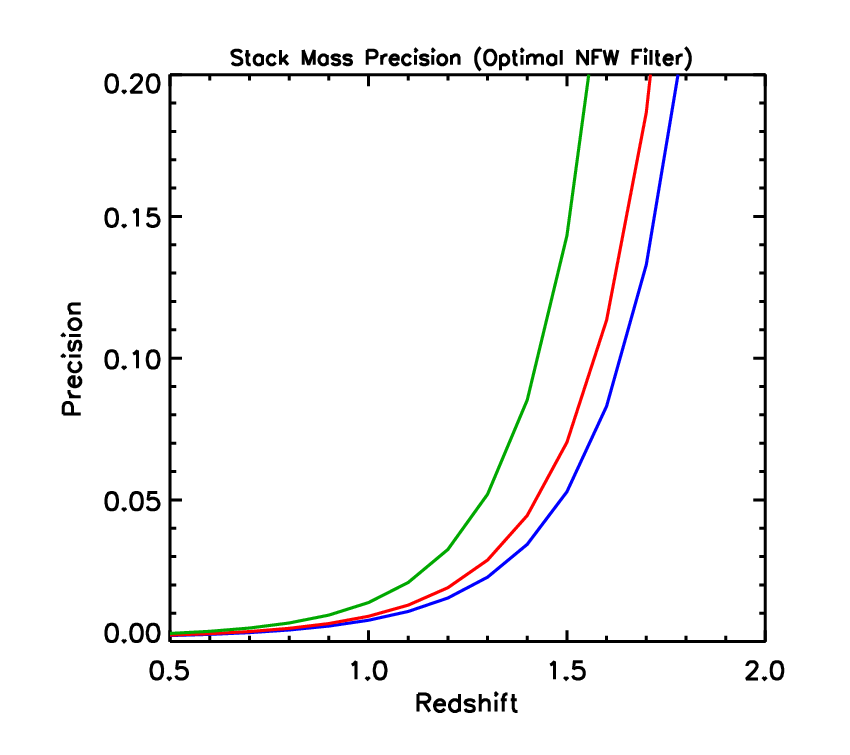
The second avenue, that represents the strength of the Euclid mission, consists in exploiting internal Euclid data. Many photometrically selected clusters will appear as signal-to-noise peaks in the Euclid full-sky cosmic shear maps. This weak gravitational lensing signal will permit us to estimate the cluster masses without relying on assumptions about dynamical equilibrium. Although only the more massive systems will permit individual mass measurements, we can nevertheless statistically calibrate the normalisation of the cluster scaling relations down to the lowest masses in the catalogue by stacking. An example is given in Fig. 12, showing the level of precision expected on the mean mass of stacked clusters.
We first measure the mass of individual clusters with a matched filter, assuming that the mass density profile of all clusters follows an NFW profile. We then calculate the uncertainty on the mean mass of the individual measurements in bins of mass () and redshift (). This result depends on the number of clusters expected in each bin, and for this purpose we have adopted the Planck cosmology (Planck Collaboration et al., 2014a) and a Euclid survey of 15,000 square degrees. The figure only accounts for shape-noise, with .
The three curves trace the precision on the mean for mass bins centred
at , , and
(from top to bottom) as a function of
redshift. We do better on the lower mass systems because their larger
number compensates for their lower individual signal-to-noise
measurements. The figure demonstrates that Euclid has the potential to
calibrate the mean mass, and hence scaling relations, to 1% out to
redshift unity, and to 10% out to
for clusters of .
At the same time, the spectroscopic part of the Euclid survey will provide velocities for a few cluster members in each cluster detected with photometric data. Stacking these velocities for many clusters in bins of richness and redshift will allow a precise calibration of the velocity dispersion vs. richness relation, and from this of the mass-richness relation.
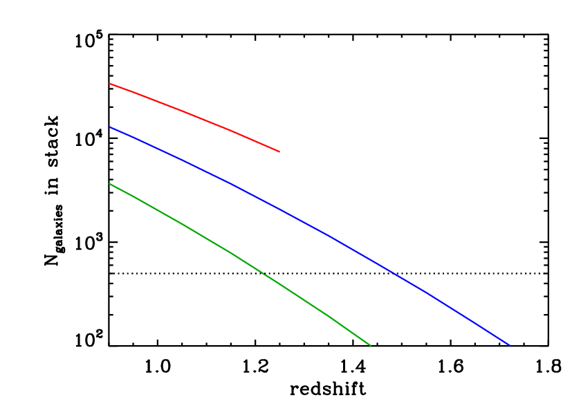
In Fig. 13, we show the number of spectroscopic cluster members that will be available for stacks of clusters of given mass in bins of and (even if, in reality, the stacking procedure will be based on mass proxies, such as richness). These numbers are evaluated using the spectroscopic selection function (bottom panel of Fig. 10), and the expected number of clusters above a given mass in our adopted cosmology, by considering only clusters with at least 5 members with redshifts. In the figure we show the predictions for three cluster masses, . The curve for is limited to because of our choice of considering only clusters with . Note that the curve for (not shown) would be limited to (and it would be lie in between those for 14.2 and 14.4).
From the analysis of Biviano et al. (2006) we find that the statistical noise
in the velocity dispersion estimate of a sample of cluster
members is per cent, which translates into a per
cent statistical noise in the mass estimate. A similar figure has been
obtained by Mamon, Biviano & Boué (2013) when using the full velocity distribution to
constrain cluster masses. The value of 500 is displayed in
Fig. 13, and it shows that a very precise spectroscopic
calibration of cluster masses will be possible for stacks of clusters
with over the redshift
range , and even beyond that ()
for clusters with masses . Spectroscopic calibration of cluster masses at higher redshifts
will be feasible with reduced precision, but lack of statistics will
hamper cluster mass calibration at .
The wide Euclid survey will allow precise calibration of the mass-observable relation out to , using gravitational lensing and spectroscopy. The deep Euclid survey will allow to extend this calibration to even higher redshifts, although with a much more limited statistics on the number of clusters. Overall, by combining Euclid internal mass calibration with the cross correlation with external SZ and X-ray surveys, we should be able to significantly mitigate the degrading effect of the nuisance parameters on cosmological constraints.