Monotonicity and Condensation in Homogeneous Stochastic Particle Systems
Abstract.
We study stochastic particle systems that conserve the particle density and exhibit a condensation transition due to particle interactions. We restrict our analysis to spatially homogeneous systems on finite lattices with stationary product measures, which includes previously studied zero-range or misanthrope processes. All known examples of such condensing processes are non-monotone, i.e. the dynamics do not preserve a partial ordering of the state space and the canonical measures (with a fixed number of particles) are not monotonically ordered. For our main result we prove that condensing homogeneous particle systems with finite critical density are necessarily non-monotone. On finite lattices condensation can occur even when the critical density is infinite, in this case we give an example of a condensing process that numerical evidence suggests is monotone, and give a partial proof of its monotonicity.
1. Introduction
We consider stochastic particle systems which are probabilistic models describing transport of a conserved quantity on discrete geometries or lattices. Many well known examples are introduced in [1], including zero-range processes and exclusion processes, which are both special cases of the more general family of misanthrope processes introduced in [2]. We focus on spatially homogeneous models with stationary product measures and without exclusion restriction, which can exhibit a condensation transition that has recently been studied intensively.
A condensation transition occurs when the particle density exceeds a critical value and the system phase separates into a fluid phase and a condensate. The fluid phase is distributed according to the maximal invariant measure at the critical density, and the excess mass concentrates on a single lattice site, called the condensate. Most results on condensation so far focus on zero-range or more general misanthrope processes in thermodynamic limits, where the lattice size and the number of particles diverge simultaneously. Initial results are contained in [3, 4, 5], and for summaries of recent progress in the probability and theoretical physics literature see e.g. [6, 7, 8]. Condensation has also been shown to occur for processes on finite lattices in the limit of infinite density, where the tails of the single site marginals of the stationary product measures behave like a power law [9]. In general, condensation results from a heavy tail of the maximal invariant measure [10], and so far most studies focus on power law and stretched exponential tails [11, 12]. As a first result, we generalize the work in [9] and provide a characterization of condensation on finite lattices in terms of the class of sub-exponential tails that has been well studied in the probabilistic literature [13, 14, 15, 16]. This characterization holds for a particular definition of condensation given in Section 2.1, which was also used in [9]. Our main result is that all spatially homogeneous processes with stationary product measures that exhibit condensation on finite lattices with a finite critical density are necessarily non-monotone.
Monotone (attractive) particle systems preserve the partial order on the state space in time, which enables the use of powerful coupling techniques to derive rigorous results on large scale dynamic properties such as hydrodynamic limits (see [17] and references therein). These techniques have also been used to study the dynamics of condensation in attractive zero-range processes with spatially inhomogeneous rates [18, 19, 20, 21, 22], and more recently [23, 24]. As we discuss in Appendix A, non-monotonicity in homogeneous systems with finite critical density can be related, on a heuristic level, to convexity properties of the canonical entropy. For condensing systems with zero-range dynamics, it has been shown that this is related to the presence of metastable states, resulting in the non-monotone behaviour of the canonical stationary current/diffusivity [25]. This corresponds to a first order correction of a hydrodynamic limit leading to an ill-posed equation with negative diffusivity in the case of reversible dynamics. Heuristically, this is of course consistent with the concentration of mass in a small, vanishing volume fraction, but poses great technical difficulties to any rigorous proof of hydrodynamic limits for such particle systems. First results in this direction only hold for sub-critical systems under restrictive conditions [26], and due to a lack of monotonicity there are no results for non-reversible dynamics.
Condensing monotone particle systems would, therefore, provide interesting examples of homogeneous systems for which coupling techniques could be used to derive stronger results on hydrodynamic limits. However, our result implies that this is not possible for condensing models with stationary product measures and a finite critical density on finite lattices. In the thermodynamic limit condensation has been defined through the equivalence of ensembles, which can be established in generality for a class of long-tailed distributions with a finite critical density [10, 7]. This class has also been studied before [14, 15] and includes the class of sub-exponential distributions, for which our results apply also in the thermodynamic limit. A detailed discussion of their connections and the resulting differences between condensation on finite lattices and in the thermodynamic limit is given in Sections 4.1 and 4.2. We remark that for systems where the dynamics is directly defined on infinite lattices there are no rigorous results or characterizations of condensation to our knowledge, and we do not discuss this case here.
For systems with infinite critical density condensation can still occur on finite lattices, and since non-monotonicity typically occurs above the critical density, such processes can also be monotone. When the tail of the stationary measure is a power law and decays faster than with the occupation number , we prove that the process is still non-monotone. In Section 5 we present preliminary results for tails that decay slower than , which strongly suggests that a monotone and condensing particle system exists (see [27] for further discussion).
The paper is organised as follows. In Section 2 we introduce the background used to study condensation and monotonicity in particle systems, and state our main results. In Section 3 we prove our main theorem by induction over the size of the lattice, showing that the family of canonical stationary measures is necessarily not monotonically ordered in the number of particles.
In Section 4 we discuss the differences between condensation on fixed lattices and in the thermodynamic limit, and prove equivalence of condensation on finite lattices with the tail of the maximal invariant product measure being sub-exponential.
In Section 5 we review examples of homogeneous processes that have been shown to exhibit condensation, and present some explicit computations for misanthrope processes and processes with power law tails.
2. Notation and results
2.1. Condensing stochastic particle systems
We consider stochastic particle systems on fixed finite lattices , which are continuous-time Markov chains on the countable state space . For a given configuration the local occupation, for , is a priori unbounded. The jump rates from configuration to are denoted , and the dynamics of the process is defined by the generator
| (2.1) |
for all continuous functions . We assume the process conserves the total number of particles
and conditioned on , the process is assumed to be irreducible, so that is the only conserved quantity. The process is therefore ergodic on the finite state space for all fixed . On the process has a unique stationary distribution , and the family is called the canonical ensemble.
We focus on systems for which the stationary distributions are spatially homogeneous, i.e. the marginal distributions are identical for all . This typically results from translation invariant dynamics on translation invariant lattices with periodic boundary conditions, but the actual details of the dynamics are not needed for our results. For these systems we define condensation in terms of the maximum occupation number
| (2.2) |
Definition 2.1.
A stochastic particle system with canonical measures on with exhibits condensation if
| (2.3) |
This condition implies in particular the existence of all limits involved. The interpretation of (2.3) is that due to the sub-exponential tails of the measure, in the limit all but finitely many particles concentrate in a single lattice site and that the distribution of particles outside the maximum is non-degenerate. As we will see in Proposition 2.3 below, the latter is in fact given by the maximal invariant measure when the system exhibits product stationary measures.
There are of course other possible definitions of condensation which are less restrictive or more appropriate in other situations. For inhomogeneous systems or thermodynamic limits (with ) the condensed phase can be localized in particular sites or have a more complicated spatial structure (see e.g. [28] and for recent summaries [7, 6, 8]). For our case of spatially homogeneous systems on finite lattices, with fixed , the above is the most convenient definition and has been used in previously studied examples [9]. A more detailed discussion is provided in Section 4.
2.2. Monotonicity and product measures
We use the natural partial order on the state space given by if and only if for all . A function is said to be increasing if implies . Two measures on are stochastically ordered with , if for all increasing functions we have , where denotes the expectation of with respect to .
A stochastic particle system on with generator and semi-group is called monotone (attractive) if it preserves stochastic order in time, i.e.
Coupling techniques for monotone processes are an important tool to derive rigorous results on the large scale dynamics of such systems such as hydrodynamic limits. There are sufficient conditions on the jump rates (2.1) to ensure monotonicity for a large class of processes (see e.g. [17] for more details), however for our results we only need a simple consequence for the stationary measures of the process.
Lemma 2.2.
If the stochastic particle system as defined in Section 2.1 is monotone, then the canonical distributions are ordered in , i.e.
| (2.4) |
The proof is completely standard but short, so we include it for completeness.
Proof.
Fix a monotone process as defined in Section 2.1. Consider two initial distributions and , concentrating on and respectively, given by
for and . Clearly , and so by monotonicity of the process this implies for all . Furthermore, by ergodicity we have
∎
All rigorous results on condensing particle systems so far have been achieved for processes which exhibit stationary product measures, for which the measures take a simple factorized form. These can then be expressed in terms of un-normalized single-site weights , . Due to conservation of such processes exhibit a whole family of stationary homogeneous product measures
| (2.5) |
The measures are defined whenever the normalization
| (2.6) |
is finite. This is the case for all fugacity parameters where or , and
| (2.7) |
is the radius of convergence of (2.6). The family is also called the grand-canonical ensemble and the (grand-canonical) partition function. Since the process is irreducible on for all we have for all . The canonical distribution can be written as
| (2.8) |
which is independent of the choice of . Equivalently
| (2.9) |
is the (canonical) partition function. Note that throughout the paper we characterize all measures by their mass functions since we work only on a countable state space and the measures concentrate on finite state spaces , which is the framework we rely on in this paper.
2.3. Results
Our results hold for systems with general stationary weights, for each , subject to the regularity assumption that
| (2.10) |
exists, which is then necessarily equal to . If then weights that satisfy (2.10) are sometimes called long-tailed [29], which is discussed in more detail in Section 4.2.
For processes with such stationary product measures there is a simple equivalent characterization of condensation which we prove in Section 4.3.
Proposition 2.3.
Consider a stochastic particle system as defined in Section 2.1 with stationary product measures as defined in Section 2.2 satisfying regularity assumption (2.10). Then the process exhibits condensation according to Definition 2.1 if and only if , , and
| (2.11) |
In this case, the distribution of particles outside of the maximum converges weakly (equivalently in total variation) to the critical product measure , i.e. for fixed we have
| (2.12) |
Note that for we may rescale the exponential part of the weights to get and we can further multiply with a constant, so that in the following we can assume without loss of generality that
| (2.13) |
The condition (2.11) can also be written as
| (2.14) |
where is the convolution product. This is a standard characterization to define the class of sub-exponential distributions (see e.g. [30, 31]). Sub-exponentiality implies that a large sum of two random variables is typically realized by one of the variables taking a large value (see Section 4.1 for more details), which is of course reminiscent for the concept of condensation. Implications and simpler necessary conditions on which imply (2.14) have been studied in detail, and we provide a short discussion in Section 4. As a consequence of Proposition 2.3, condensation is only a property of the tail of , therefore if a process with stationary product measures (2.9) condenses in the sense of Definition 2.1 for some , it condenses for all .
Proposition 2.3 provides a generalization of previous results on condensation on finite lattices [9] and is used in the proof of our main result, which is the following.
Theorem 2.4.
Consider a spatially homogeneous stochastic particle system as defined in Section 2.1 which exhibits condensation in the sense of Definition 2.1, has stationary product measures that satisfy (2.10), and has finite critical density
| (2.15) |
then the process is necessarily not monotone.
The same is true if (2.15) is replaced by the assumption that11
1
For functions we use the notation if as .
with .
2.4. Discussion
The class of distributions which fulfil (2.11) (called sub-expontial), and therefore exhibit condensation on finite lattices, is large (see e.g. [13, Table 3.7]), and includes in particular
- •
power law tails where ,
- •
log-normal distribution
(2.16) where and , which always has finite mean,
- •
stretched exponential tails for , ,
- •
almost exponential tails for .
For the last two examples all polynomial moments are finite. This covers all previously studied models on condensation in zero-range processes [5, 9, 12]. As we will discuss in Section 4.2 all these examples also exhibit condensation in the thermodynamic limit, whenever they have finite first moment. It can also be shown that the limit in (2.14) is necessarily equal to and that in fact for any fixed (see [16] and Proposition 3.2).
Since we consider a fixed lattice , is not a necessary condition for condensation as opposed to systems in the thermodynamic limit. Even if the distribution of particles outside the maximum has infinite mean, condensation in the sense of Definition 2.1 can occur. However, if (e.g. for power law tails with ), the distribution of particles outside the maximum cannot be normalized, condition (2.11) fails, and there is no condensation in the sense of our definition.


We will prove non-monotonicity in the next section by showing that expectations for a particular monotone decreasing observable under are not decreasing in . The chosen function is related to (but not equal to) the number of particles outside the maximum (condensate), which has been shown previously to exhibit non-monotone behaviour for a class of condensing zero-range processes in the thermodynamic limit [25, 12]. When the number of particles just exceeds the critical value, typical configurations still appear homogeneous with a maximum occupation number of22 2 For functions we use the notation if as . . Only when the number of particles is increased further the system switches to a condensed state with a maximum that contains a non-zero fraction of all particles. We present numerical evidence of this non-monotone switching behaviour for the background density
| (2.17) |
in Figure 1. This is a finite size effect which disappears in the limit , and for specific models it has been shown to be related to the existence of super-critical homogeneous metastable states [25, 12, 32]. For large , the switching to condensed states occurs abruptly over a relatively small range of values for . Since the are conditional product measures the correlations in the system are very weak, which causes metastable hysteresis effects and non-monotonicity of the canonical ensemble around the critical point. Metastable hysteresis has been established in [25, 12] for zero-range processes. Our result implies that this behaviour is generic for all condensing systems with finite critical density. We also give a heuristic discussion of the connection to convexity properties of the entropy of the system in Appendix A.
There are several examples of homogeneous, condensing, monotone particle systems with finite critical density which have been studied on a heuristic level and which we summarize in Section 5. Their stationary measures are not of product form and no explicit formulas are known, so these systems are therefore hard to analyse rigorously. For systems with non-product stationary measures, upward fluctuations in the density which are homogeneously distributed may be suppressed strongly enough, so that the metastable states do not exist. Such models may then also be monotone, and examples are given in Section 5.3.
We excluded the case in the presentation in Section 2.3 for notational convenience, but it is easy to see that our results also hold in this case. With the convention we have and , and then existence of the limit is equivalent to
i.e. condensation of all particles on a single site. This can easily be extended to all with Proposition 3.2. Considering only events with all particles on one site, or particles on one site and particle elsewhere, we have convergence from above
This implies the non-monotonicity of as discussed in Section 3.
3. Proof of Theorem 2.4
We assume that the process exhibits condensation in the sense of Definition 2.1 and has stationary product measures, so the canonical measures are of the form (2.9). Furthermore, we assume the weights satisfy the regularity assumption, and without loss of generality , see (2.13). We show that the family of canonical measures is not stochastically ordered in , which implies non-monotonicity of the process by Lemma 2.2. To achieve this, we use the test function
| (3.1) |
which indicates the event where all particles concentrate in the maximum at site .
Lemma 3.1.
The function defined in (3.1) is monotonically decreasing, which implies that
| (3.2) |
whenever the family of canonical measures is stochastically ordered in .
Proof.
Fix configurations such that . If then has at least one particle outside of site , therefore so does which implies . If then necessarily since . Therefore is a decreasing function. Using (2.9) and the convention (2.13), we find that the canonical expectation of the function (3.1) is given by
So if the canonical measures are monotone in , monotonicity of implies (3.2). ∎

By Proposition 2.3 we know that for condensing systems the ratio converges. This implies the sequence in Lemma 3.1 converges, as summarised in the following proposition using our notation (see [16, Theorem 1 and Lemma 5]).
Proposition 3.2.
Note that the limit in (3.3) states that the probability of observing a large total number of particles under the critical product measure is asymptotically equivalent to the probability of observing a large number of particles on any one of the sites, precisely
This is further equivalent to the canonical probability of the maximum containing the total mass converges to the critical probability that sites are empty, i.e. .
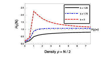
To complete the proof we show that a subsequence of converges from above, which contradicts the assumption of monotonicity by Lemma 3.1. We present a numerical illustration for the monotonicity properties of the function
| (3.4) |
in Figure 2, which is normalized such that as . The proof of the following lemma represents the most significant part of the proof of Theorem 2.4 and is given in Section 3.1 for the case of finite mean and in Section 3.2 for the power law case.
Lemma 3.3.
Under the conditions of Theorem 2.4, and assuming without loss of generality , for each there exists a and a sequence with as such that
Therefore, we know that there exists some such that , which by Lemma 3.1 implies that the canonical measures are not stochastically ordered in , and thus the process cannot be monotone by Lemma 2.2. This completes the proof of Theorem 2.4.
3.1. Proof of Lemma 3.3: The finite mean case
In order to prove that converges from above for some non-decreasing sequence we first specify a sequence on which we can bound the ratio below.
Claim 3.4.
For weights with finite and non-zero first moment, i.e. , there exists a sequence with as such that for all
| (3.5) |
Proof.
For each , define as follows
By definition is a non-decreasing sequence. Assume for contradiction that is bounded above, then for all we would have for some , and therefore contradicting the assumption of finite first moment. For we have
∎
Claim 3.5.
For weights with finite first moment, there exists a subsequence of the sequence defined in Claim 3.4 such that for all and sufficiently large.
Proof.
By neglecting at most a single term in the sum defining , the ratio can be bounded below as follows,
| (3.6) |
We define
to be the largest index where the ratio is minimized. In particular
| (3.7) |
By definition , and so . There exists a subsequence such that , with a slight abuse of notation we denote the subsequences and simply by and . Suppose , by Claim 3.4 we have
which together with (3.7) contradicts Proposition 3.2, therefore and for all .
To complete the proof of Lemma 3.3 we proceed by induction on the system size, . We make the following inductive hypothesis;
- (H)
there exists a sequence such that for all and sufficiently large.
The case is given by Claim 3.5. Analogously to the proof of Claim 3.5 we define
| (3.9) |
By the same argument as in the proof of Claim 3.5 there exists a subsequence such that , again we denote the respective subsequences by and . For sufficiently large, we have
where the final inequality follows from the inductive hypothesis (H) and Claim 3.4. Subtracting we get
| (3.10) |
Now, following the proof of Claim 3.5, multiply (3.10) by and neglect the second term on the second line. Then the first term vanishes, since
In terms of the normalized grand-canonical measure , so we have
| (3.11) |
where is the critical density as defined in (2.15). This implies that the first term in the second line of (3.10), after multiplication with , converges to a strictly positive constant. Finally, the third line in (3.10) converges to zero after multiplying by since we have , which implies
as , by (3.11). Using the definition of in (3.9), this implies that there exists a constant such that for all large enough
so (H) holds for , completing the induction. This concludes the proof of Lemma 3.3 for the case where the critical measure has finite mean.
3.2. Proof of Lemma 3.3: The infinite mean power law case
We consider stationary weights of the form with , , and . We prove non-monotonicity of for and for all via an exact computation. The case can be done completely analogously but involves different expressions with logarithms in the resulting limits, and is presented in Appendix B. The proof remains valid for general converging with only minor differences, which we explain in a remark at the end of this section. Convergence of from above or below for the exact power law depends on the parameter , as summarized in the next result.
Lemma 3.6.
For stationary weights of the form and with
| (3.12) |
where
For we have
| (3.13) |
which has the same sign as .
This result implies that whenever for and with Lemma 3.3 holds with . This completes the proof of Lemma 3.3 in the case .
Proof of Lemma 3.6.
To prove this result we make use of the full Taylor series of at and integral approximations to compute the asymptotic behaviour of summations. To simplify notation we assume that is even. For odd there is no term with multiplicity one and there exists an obvious modification. First note that fulfils the regularity assumption (2.13) and as for all [9], so by Proposition 2.3 a process with stationary measures will exhibit condensation. For we subtract from to get
| (3.14) |
Substituting the Taylor expansion of we find
| (3.15) |
In the last line the term was combined with the second term, and we adopt the usual convention that empty products are equal to one. Both summations in are over continuous and monotone functions , therefore we can use the usual integral approximation for decreasing (increasing) functions
| (3.16) |
for all and . Multiplying by we find the limit as of (3.15) to be
| (3.17) |
It is shown in Appendix C that this is positive (and finite) in the region and negative (and finite) in the region , completing the proof of Lemma 3.6 for . The result holds for general system size, , and is proved by induction. The inductive hypothesis states
| (3.18) |
Similar to the case we write
| (3.19) |
We first establish the limit of the function in equation (3.19). The inductive hypothesis (3.18) can be written as
| (3.20) |
which implies can be written as
Rearranging terms and noting that we then have
After Taylor expanding appearing in the first line above, it is easy to see that the limit of the first line is given by as . Using the result to calculate the limit of the second line we find
| (3.21) |
To identify the limit of in (3.19), we again make use of the Taylor expansion of similarly to the two site case and we write
Changing the order of summations, separating the term and using we have
| (3.22) |
For all and we have as , which implies that for any fixed we have . Therefore, the following limits are equal
Using the inductive hypothesis (3.20) we have is given by
| (3.23) |
Now applying the result it is possible to show that
| (3.24) |
where the limit of the first line of (3.23) was by the additional factor appearing in the summations. Combining (3.21) and (3.24) we have
concluding the induction so the result holds for all . From the recursion (3.13) it is obvious that will have the same sign as , completing the proof of Lemma 3.6. ∎
A slightly modified version of Lemma 3.6 also holds if the stationary weights are of the form where . The limit in (3.12) only depends on the tail behaviour of the weights and is now given by . Briefly, this can be seen as follows, (3.14) becomes
Taylor expanding and rearranging to find terms of the form and using the same argument to calculate the limit of we have
for all and any ,
and the result follows. Similar modifications are required in the inductive step and the new limit in (3.13) is given by for all . This does not change the sign of the limit in (3.13) and therefore Lemma 3.3 still holds.
4. Characterization of condensation
Condensation arises in spatially homogeneous systems with stationary product measures due to the sub-exponential tail of the stationary weights , which has been studied extensively in previous work. In this section we review relevant results on heavy-tailed distributions and discuss the links between condensation on finite fixed lattices and in the thermodynamic limit before we give the proof of Proposition 2.3 in Section 4.3.
4.1. Sub-exponential distributions
Sub-exponential distributions are a special class of heavy-tailed distributions, the following characterization was introduced in [33] with applications to branching random walks, and has been studied systematically in later work (see e.g. [16, 14, 15, 30]), for a review see for example [13] or [31].
A non-negative random variable with distribution function is called heavy-tailed if , for all , and
| (4.1) |
It is called sub-exponential if , for all , and
| (4.2) |
Here denotes the convolution product, the distribution function of the sum of two independent copies and . It has been shown [33, 34] that (4.2) is equivalent to either of the following conditions,
| (4.3) | ||||
| (4.4) |
The second characterization shows that a large sum of independent sub-exponential random variables is typically realized by one of them taking a large value, which is of course reminiscent of the condensation phenomenon. It was further shown in [33, 13] that sub-exponential distributions also have the following properties,
| (4.5) | ||||
| (4.6) | ||||
| (4.7) |
Most results in the literature are formulated in terms of distribution functions and tails and apply to discrete as well as continuous random variables. [16] provides a valuable connection to discrete random variables in terms of their mass functions , .
Assume the following properties for a sequence ,
- (a)
as ,
- (b)
(normalizability),
- (c)
exists.
Then [16, Theorem 1] asserts that and is the mass function of a discrete, sub-exponential distribution. The implication
is given in [16, Lemma 5]. Sufficient (but not necessary) conditions for assumption (c) to hold are given in [16, Remark 1].
Provided , then (c) holds if either of the following conditions are met:
- (i)
for some constant , or
- (ii)
where is a smooth function on with and as , and .
Case (i) includes distributions with power law tails, with . The stretched exponential with , , and the almost exponential with , , are covered by case (ii). The class of sub-exponential distributions includes many more known examples than the list given in Section 2.4 (see e.g. [13, Table 3.7]).
Analogous to the characterisation of sub-exponential distributions, given by (4.4), for discrete distributions the existence of the limit is equivalent to the existence of the following condition
| (4.8) |
This holds, since we have the following equality of ratios
Specific properties of power law tails are used in [9] to show condensation for finite systems in the sense of Definition 2.1. In Proposition 2.3, proved in Section 4.3, we extend this result to stationary product measures with general sub-exponential tails. In this context, condensation is basically characterized by the property (4.4) which assures emergence of a large maximum when the sum of independent variables is conditioned on a large sum. As summarized in the introduction, condensation in stochastic particle systems has mostly been studied in the thermodynamic limit with particle density , where such that . In that case conditions on the sum of independent random variables become large deviation events, which have been studied in detail in [35, 36].
4.2. Connection with the thermodynamic limit
In the thermodynamic limit, a definition of condensation is more delicate and the approach presented in [10, 7] follows the classical paradigm for phase transitions in statistical mechanics via the equivalence of ensembles (see e.g. [37] for more details). A system with stationary product measures (2.5) exhibits condensation if the critical density (2.15) is finite, i.e. and the canonical measures are equivalent to the critical product measure in the limit such that for all super-critical densities . The interpretation is again that the bulk of the system (any finite set of sites) is distributed as the critical product measure in the limit. It has been shown in [10] (see also [7] for a more complete presentation) that the regularity condition (2.10) and imply the equivalence of ensembles, which has therefore been used as a definition of condensation in [7, Definition 2.1]. Therefore, any process that condenses for fixed with in the sense of Definition 2.1 also condense in the thermodynamic limit. This includes all previously studied examples [5, 9, 12], however there exists distributions that satisfy (2.10) with but do not satisfy the conditions of Proposition 2.3 and do not condense for fixed . This is illustrated by an example given below. It is also discussed in [7, Section 3.2] that assumption (2.10) is not necessary to show equivalence, but weaker conditions are of a special, less general nature and are not discussed here. Note also that equivalence of ensembles does not imply that the condensate concentrates on a single lattice site, the latter has been shown so far only for stretched exponential and power-law tails with in [11, 12]. Both definitions involve only the sequence of canonical measures and not on the dynamics of the underlying process. Since the canonical measures (2.9) are fully characterised by the weights condensation can be viewed as a feature of the tails of the weights .
The condensation phenomena can also be studied for continuous random variables on the local state space , see for example [36]. The following continuous example, taken from [15] is shown to satisfy (2.10) but is not sub-exponential. We show that the distribution has a finite mean and therefore exhibits condensation in the thermodynamic limit but not on a finite lattice in the sense of Definition 2.1. For a real-valued random variable with distribution function , assume . Let to be an increasing sequence with and be a continuous and piecewise linear function such that and for . The sequence is defined iteratively as follows
and for . The mean is finite since
where the final step uses the relation to bound the series from above.
For all distributions satisfying (2.10) which are not sub-exponential does not have a limit in as and with Proposition 2.3 there is no condensation on finite lattices according to Definition 2.1. For a discretized version of the example given above with weights we have for as [15]. For this example, following the proof of Proposition 2.3 this implies that for as and all . Therefore, the bulk occupation number diverges in distribution as by receiving a diverging excess mass from the condensate due to the light tail of . It can be shown that these weights satisfy (2.10) and therefore exhibit condensation in the thermodynamic limit where the excess mass can be distributed on a diverging number of sites.
For a process that exhibits condensation in the thermodynamic limit with a sub-exponential critical product measure, Proposition 2.3 implies that condensation occurs also on finite lattices with . Theorem 2.4 then implies that this process is necessarily non-monotone for all fixed system sizes . However, monotonicity for condensing processes with long-tailed but not sub-exponential stationary measures remains open.
4.3. Proof of Proposition 2.3
Let us first assume that the process exhibits condensation according to Definition 2.1 and has canonical distributions of the form (2.9) where the weights fulfil (2.10), i.e. as . In this part of the proof we establish that;
- (1)
,
- (2)
has a limit as ,
- (3)
, which also implies as , and
- (4)
convergence of for some implies convergence for and therefore (2.11) holds.
Step (1), show . Assume first that as . For all and we have
Let . The partition function is trivially bounded below by the event that site 1 takes particles and the second site takes the remaining particles, i.e.
Therefore
as , which implies condensation cannot occur in the sense of Definition 2.1 contradicting the initial assumption, therefore .
Step (2), prove converges as . By Definition 2.1 the limit
| (4.9) |
exists and for sufficiently large. For we have
| (4.10) |
Since , is fixed, and , (4.10) implies the convergence of as .
Step (3), prove . By (2.3) we have as , taking the limit as of (4.10) this implies
| (4.11) |
Since we also have , this implies . Using , (4.10) then also implies as .
Step (4). We have seen above that condensation implies , , and as , then [38, Theorem 2.10] implies
completing this part of the proof.
Now, let us consider a stochastic particle system with canonical distributions of the form (2.9) which fulfil (2.13) and (2.14) with and . We keep the notation for general in the following to clarify the argument. It is immediate from Proposition 3.2, and remembering that we set , that
Then we have for all fixed and
as . Since is a non-degenerate probability distribution, this implies that as , which is (2.3).
5. Examples of homogeneous condensing processes
In this section we review several stochastic particle systems that exhibit condensation. By Theorem 2.4, if these processes are homogeneous and monotone with a finite critical density they do not have stationary product measures.
To prove monotonicity for the examples mentioned below it is sufficient to construct a basic coupling of the stochastic process which preserves the partial order and particles jump together with maximal rate.
For a definition of a coupling see [39] and for the statement of Strassen’s theorem linking stochastic monotonicity and the coupling technique see [40].
The steps to construct a basic coupling are outlined in [17].
5.1. Misanthrope processes and generalizations
Condensation in homogeneous particle systems has mostly been studied in the framework of misanthrope processes [2, 17]. At most one particle is allowed to jump at a time and the rate that this occurs depends on the number of particles in the exit and entry sites. The misanthrope process is a stochastic particle system on the state space defined by the generator
| (5.1) |
Here denotes the configuration after a single particle has jumped from site to site , which occurs with rate . The purely spatial part of the jump rates, , are transition probabilities of a random walk on . Such models are usually studied in a translation invariant setting with periodic boundary conditions, typical choices are symmetric, totally asymmetric or fully connected jump rates with , , or , respectively.
Misanthrope processes include many well-known examples of interacting particle systems, such as zero-range processes [1], the inclusion process [41, 42], and the explosive condensation model [43]. It is known [2, 27] that misanthrope processes with translation invariant dynamics exhibit stationary product measures if and only if the rates fulfil
| (5.2) |
and, in addition, either
| (5.3) |
The corresponding stationary weights satisfy
| (5.4) |
Misanthrope processes are monotone (attractive) [2] if and only if the jump rates satisfy
| i.e. non-decreasing in , | ||||
| (5.5) |
In Theorem 2.4 we have proved that processes that exhibit stationary product measures and condensation with finite mean or power law tails, , with are necessarily not monotone. For power law tails with convergence of is from below and our method does not disprove monotonicity of the measures or monotonicity of the underlying process. Using the specific form of the stationary measures (5.4), it is clear that possible examples of monotone processes with stationary product measures of this form cannot be of misanthrope type.
Lemma 5.1.
A misanthrope process defined by the generator (5.1), that has stationary product measures and exhibits condensation is not monotone.
Proof.
(5.5) gives necessary conditions for the monotonicity of the misanthrope process and implies with (5.4) that
| (5.6) |
is non-decreasing. This implies that the ratio converges to , which is the regularity assumption (2.10). Assuming the process condenses in the sense of Definition 2.1, then Proposition 2.3 implies . Now we have
| (5.7) |
for all . Therefore, which implies
| (5.8) |
We conclude that the critical partition function diverges and the critical measure does not exist, which is a necessary condition for condensation. Therefore condensation does not occur in misanthrope processes with stationary product measures. ∎
In [17] generalised misanthrope processes have been introduced where more than one particle is allowed to jump simultaneously. They are defined via transitions for at rate and conditions on the jump rates for monotonicity are characterized. This class provides candidates for possible monotone, condensing processes with product measures as we discuss in the next subsection.
5.2. Generalised zero-range processes
The generalised zero-range process (gZRP) [17] is a stochastic particle system on the state space defined by the generator
| (5.9) |
Here is the configuration after particles have jumped from to . The jump rates satisfy if , and we use the convention that empty summations are zero. We consider translation invariant on a finite lattice and note that the process preserves particle number .
It is known [44, 27] that these processes exhibit stationary product measures if and only if the jump rates have the explicit form
| (5.10) |
where are arbitrary non-negative functions with strictly positive. The stationary weights are then given by . Monotonicity of the gZRP can be characterized in terms of
| (5.11) |
The gZRP is monotone if and only if
| (5.12) |
We note these conditions arise from a special case of the results in [17, Theorem 2.11] on generalised misanthrope models, since depends only on the occupation of the exit site and not the entry site.
In this class, which is also discussed in detail in [27], condensing processes which are monotone, homogeneous, and have stationary product measures with a power tail with are conjectured to exist. As an example, consider the gZRP with rates given by
| (5.13) |
Since is of the form (5.10) the process exhibits stationary product measures with weights of the form
For all and the ratio converges to as [9] so by Proposition 2.3 the process exhibits condensation. To prove the process is monotone we must show the rates satisfy the conditions given in equation (5.12). We first prove for all and . Since for all we can drop the term from the definition of . We have
Since is increasing in for and we have
We also need to show for all and . Taking discrete derivatives in
so is an increasing function in . Therefore,
for all , and it suffices to show
| (5.14) |
We present numerical evidence in Figure 3 which corroborates our claim that the process with rates (5.13) is indeed monotone for and is not for .

5.3. Homogeneous monotone processes without product measures
The chipping model is a stochastic particle system on the state space , introduced in [45, 46]. The dynamics are defined by the generator
| (5.15) |
Here denotes the configuration after all the particles at site have jumped to site , which occurs at rate , and single particles jump at rate . The spatial part is again spatially homogeneous as described in Section 5.1.
It is easy to see that a basic coupling will preserve the partial order on the state space as defined in Section 2.2. Therefore, by Strassen’s theorem [40], the chipping model is a monotone process and Lemma 2.2 implies that conditional stationary measures of the process are ordered in . The condensation transition in the chipping model was established on a heuristic level in [45, 46, 47]. We have defined the critical density only for systems with product stationary measures (see (2.15)). In general, the critical density on a fixed system of size , with unique invariant measures , can be defined as the background density of bulk sites
| (5.16) |
Notice if are conditional product measures (see (2.9)) then is consistent with (2.15) and in particular independent of , which follows from Proposition 2.3 (more explicitly (2.12)). For the chipping model in the case , the process reduces to a -dimensional process on and the measure and can be computed explicitly to find
| (5.17) |
In [45, 46, 47] the critical density in the thermodynamic limit is defined as
inspired by the fact that in case of condensation the second moment is either dominated by the condensate and scales like the system size , or it diverges since the maximal invariant measure does not have finite second moment. It is shown by heuristic computations in a mean-field limit that
This suggests that the critical density can depend on the system size for distributions with non-product stationary measures.
The scaling of the critical density can be intuitively understood in the two site chipping model with particles. This process can be interpreted as a symmetric random walk on the state space with jumps at rate and random jumps to either boundary (resetting, or ) at rate . After a reset the particle diffuses at rate and reaches a typical distance from the boundary until the next reset. So this model is a monotone and spatially homogeneous process that heuristically exhibits a condensation transition with finite (size dependent) critical density, but it does not exhibit stationary product measures. Condensation is also observed in models where chipping is absent () and the dynamics result in a single block of particles jumping on the lattice corresponding to the critical density .
Appendix A Connection to statistical mechanics
Condensation and non-monotonicity are also related to convexity properties of the entropy, which we briefly describe in the following in a non self-contained and non-rigorous discussion that is aimed at readers with a background in statistical mechanics. In the thermodynamic limit the canonical entropy is defined as
| (A.1) |
For the processes we consider, equivalence of canonical and grand-canonical ensembles has been established in [10] for condensing or non-condensing systems, so is given by the (logarithmic) Legendre transform of the pressure
| (A.2) |
This takes a particularly simple form since the grand-canonical measures are factorisable, and is a strictly convex function for . General results then imply that also has to be strictly convex below the critical density (see e.g. [48]), which holds for non-condensing systems and condensing systems with . For condensing systems with finite critical density is linear for , consistent with phase separation phenomena, where in this case the condensed phase formally exhibits density (see e.g. [32] for a general discussion).
It is not possible to derive general results for finite and , but if we assume that the ratio of weights is monotone increasing in , we can show that a monotone order of implies that is necessarily convex. Note that with (2.10) our assumption implies that has exponential tails with or decays super-exponentially with , and in both cases the system does not exhibit condensation. We can define so that is a monotone increasing test function on . It is easy to see that for its canonical expectation we have for all and
| (A.3) |
Therefore, monotonicity of the canonical measures implies that the ratio of partition functions (A.3) is increasing and the discrete derivative of in is decreasing. We expect that in the limit the monotonicity assumption on is not necessary, and is convex in for all non-condensing systems, consistent with strict convexity of .
For condensing systems the weights decay sub-exponentially, and if is monotone then it has to be decreasing in . Therefore the choice implies is not a monotone test function, and the above general arguments cannot be used to relate non-convexity of to the absence of a monotone order in . For particular condensing systems, however, it has been shown that is typically convex for small and concave for larger [25, 12]. These results focus on power law and stretched exponential tails for , and have been derived for zero-range processes where the ratio is equal to the canonical current. Non-monotone behaviour around the critical density therefore has implications for finite-size corrections and derivations of hydrodynamic limits as mentioned in the introduction.
Appendix B The infinite mean power law case with
Consider stationary weights of the form with , we prove the non-monotonicity of in a similar fashion to the proof of Lemma 3.6 summarised in the following lemma.
Lemma B.1.
For stationary weights of the form with we have
For we have
| (B.1) |
which is positive for all since .
Proof.
First consider the case . As in the proof of Lemma 3.6 we will utilise the full Taylor expansion of , integral bounds on monotone series, and assume is even, for odd there exists obvious modifications to the proof. We have
Where the terms in the above summations cancel. Substituting the Taylor expansion of we find
| (B.2) |
Now we are in a position to apply the integral bounds (3.16), first noting that is decreasing for , constant and equal to for , and increasing for . Multiplying both sides of (B.2) and applying the integral bounds it is easy to show
Now consider the case and make the following inductive hypothesis
As in the proof of Lemma 3.6 write
| (B.3) |
We fist establish the limit of in (B.3). The inductive hypothesis can be rewritten as
| (B.4) |
Similar to the proof of Lemma 3.6 can be written in the form
| (B.5) |
Since is decreasing for we can find upper and lower bounds of the first term, by pulling out the logarithm, of the form
Applying the same steps exactly as they appear in the proof of Lemma 3.6 to the upper and lower bounds we have
| (B.6) |
To identify the limit of in (B.3) we again follow the steps given in the proof of Lemma 3.6, which implies
| (B.7) |
Combining this with (B.6) we have
From the recursion (B.1) it is obvious that will have the same sign as , completing the proof of Lemma B.1.
∎
Appendix C On the sign of
In this section, we compute the sign of for , where
Recall the definition of the Pochhammer symbol
and the hypergeometric function
We now show
| (C.1) |
which in particular implies by evaluating the hypergeometric formula. Factorising the term from and rearranging terms inside the summation we have
Now use the following identities to simplify the terms inside the summation
which gives the required result (C.1).
To complete the proof we use the following two relations for hypergeometric functions, Euler’s transform [49, 15.3.3]
and Gauss’s second summation theorem [49, 15.1.24]
Therefore,
To calculate the sign of we first note that the gamma function is positive for all and negative in the region , which implies
Acknowledgements
This work was supported by the Engineering and Physical Sciences Research Council (EPSRC), Grant No. EP/101358X/1. P.C. acknowledges fellowship funding from the University of Warwick, Institute of Advanced Study. The authors are grateful to Ellen Saada and Thierry Gobron for useful discussions and comments on the manuscript.
References
- [1] (1970) Interaction of Markov processes. Adv. Math. 5, pp. 246–290. Cited by: §1, §5.1.
- [2] (1985) Processus des misanthropes. Z. Wahrscheinlichkeitstheorie 70 (4), pp. 509–523. External Links: ISSN 0044-3719, Link Cited by: §1, §5.1, §5.1, §5.1.
- [3] (1998) A simple stochastic model for the dynamics of condensation. J. Phys. A-Math. Gen. 31 (1), pp. L19. External Links: ISSN 0305-4470, Link Cited by: §1.
- [4] (2000) Size of the largest cluster under zero-range invariant measures. Ann. Probab. 28 (3), pp. 1162–1194. External Links: Link Cited by: §1.
- [5] (2000) Phase transitions in one-dimensional nonequilibrium systems. Braz. J. Phys. 30 (1), pp. 42–57. External Links: ISSN 0103-9733, Link Cited by: §1, §2.4, §4.2.
- [6] (2012) Condensation in the inhomogeneous zero-range process: an interplay between interaction and diffusion disorder. J. Stat. Mech. Theor. Exp. (12), pp. P12013. External Links: ISSN 1742-5468, Link Cited by: §1, §2.1.
- [7] (2013) Condensation in Stochastic Particle Systems with Stationary Product Measures. J. Stat. Phys. 154 (1-2), pp. 432–465. External Links: ISSN 0022-4715 Cited by: §1, §1, §2.1, §4.2.
- [8] (2014) Condensation in stochastic mass transport models: beyond the zero-range process. J. Phys. A-Math. Theor. 47 (9), pp. 095001. External Links: ISSN 1751-8113, Link Cited by: §1, §2.1.
- [9] (2007) Condensation for a Fixed Number of Independent Random Variables. J. Stat. Phys. 128 (5), pp. 1153–1158. External Links: ISSN 0022-4715, Link Cited by: §1, §2.1, §2.3, §2.4, §3.2, §4.1, §4.2, §5.2.
- [10] (2003) Condensation in the Zero Range Process: Stationary and Dynamical Properties. J. Stat. Phys. 113 (3-4), pp. 389–410. External Links: ISSN 0022-4715, Link Cited by: Appendix A, §1, §1, §4.2.
- [11] (2008) Thermodynamic limit for the invariant measures in supercritical zero range processes. Probab. Theory Relat. Fields 145 (1-2), pp. 175–188. External Links: ISSN 0178-8051, Link Cited by: §1, §4.2.
- [12] (2013) Zero range condensation at criticality. Stoch. Proc. Appl. 123 (9), pp. 3466–3496. External Links: Link Cited by: Appendix A, §1, §2.4, §2.4, §2.4, §4.2.
- [13] (1998) Subexponential Distributions. In A pract. guid. to heavy tails stat. tech. anal. heavy tailed distrib., pp. 435–459. External Links: Link Cited by: §1, §2.4, §4.1, §4.1, §4.1.
- [14] (1975) The Class of Subexponential Distributions. Ann. Probab. 3, pp. 1000–1011. External Links: ISSN 0091-1798 Cited by: §1, §1, §4.1.
- [15] (1980) Subexponential distribution functions. J. Austral. Math. Soc. Ser. A 29, pp. 337–347. External Links: Link Cited by: §1, §1, §4.1, §4.2, §4.2.
- [16] (1973) Functions of probability measures. Journal d’analyse mathématique 26 (1), pp. 255–302. Cited by: §1, §2.4, §3, §4.1, §4.1, §4.1, §4.1.
- [17] (2010) Couplings, attractiveness and hydrodynamics for conservative particle systems. Ann. I. H. Poincare-PR 46 (4), pp. 1132–1177. External Links: ISSN 0246-0203, Link Cited by: §1, §2.2, §5.1, §5.1, §5.2, §5.2, §5.
- [18] (1996) Phase Transitions in Driven Diffusive Systems With Random Rates. J. Phys. A-Math. Gen. 29, pp. L465–L471. Cited by: §1.
- [19] (1996) Hydrodynamical limit for space inhomogeneous one-dimensional totally asymmetric zero-range processes. Ann. Probab. 24 (2), pp. 599–638. External Links: ISSN 2168-894X, Link Cited by: §1.
- [20] (1996) Asymmetric conservative processes with random rates. Stoch. Proc. Appl. 61 (2), pp. 181–204. External Links: ISSN 0304-4149, Link Cited by: §1.
- [21] (2000) Convergence to the maximal invariant measure for a zero-range process with random rates. Stoch. Proc. Appl. 90 (1), pp. 67–81. External Links: ISSN 0304-4149, Link Cited by: §1.
- [22] (2007) Escape of mass in zero-range processes with random rates. IMS Lect. notes, Asymptotics Part. Process. Inverse Probl. 55, pp. 108–120. Cited by: §1.
- [23] (2014) Supercritical behavior of asymmetric zero-range process with sitewise disorder. pp. 48. Cited by: §1.
- [24] (2015) Supercriticality conditions for asymmetric zero-range process with sitewise disorder. Braz. J. Probab. Stat. 29 (2), pp. 313–335. External Links: ISSN 0103-0752, Link Cited by: §1.
- [25] (2010) Finite Size Effects and Metastability in Zero-Range Condensation. J. Stat. Phys. 140 (5), pp. 846–872. External Links: ISSN 0022-4715, Link Cited by: Appendix A, §1, §2.4, §2.4.
- [26] (2014) Hydrodynamic Limit of Mean Zero Condensing Zero Range Processes with Sub-Critical Initial Profiles. J. Stat. Phys. 158 (1), pp. 87–104. External Links: ISSN 0022-4715, Link Cited by: §1.
- [27] Invariant measures for mass migration processes. arXiv:1507.00778 [math.PR]. Cited by: §1, §5.1, §5.2, §5.2.
- [28] (2007) Condensation in zero-range processes on inhomogeneous networks. Phys. Rev. E 76 (4), pp. 046114. Cited by: §2.1.
- [29] (2011) An introduction to heavy-tailed and subexponential distributions. Springer. Cited by: §2.3.
- [30] (1989) Subexponential distributions and characterizations of related classes. Probab. Theory Relat. Fields 82 (2), pp. 259–269. External Links: ISSN 0178-8051, Link Cited by: §2.3, §4.1.
- [31] (2004) Subexponential Distributions - Large Deviations with Applications to Insurance and Queueing Models. Aust N Z J Stat 46 (1), pp. 145–154. External Links: ISSN 1369-1473, Link Cited by: §2.3, §4.1.
- [32] (2015) A dynamical transition and metastability in a size-dependent zero-range process. J. Phys. A-Math. Theor. 48 (5), pp. 055001. External Links: ISSN 1751-8113, Link Cited by: Appendix A, §2.4.
- [33] (1964) A Theorem on Sums of Independent Positive Random Variables and Its Applications to Branching Random Processes. Theory Probab. Appl. 9 (4), pp. 640–648. External Links: ISSN 0040-585X, Link Cited by: §4.1, §4.1, §4.1.
- [34] (1980) On closure and factorization properties of subexponential and related distributions. J. Austral. Math. Soc. Ser. A 29 (02), pp. 243–256. External Links: Link Cited by: §4.1.
- [35] (2008) Large deviations for random walks under subexponentiality: The big-jump domain. Ann. Probab. 36 (5), pp. 1946–1991. External Links: ISSN 2168-894X, Link Cited by: §4.1.
- [36] (2011) Conditional distribution of heavy tailed random variables on large deviations of their sum. Stoch. Proc. Appl. 121 (5), pp. 1138–1147. External Links: ISSN 03044149, Link Cited by: §4.1, §4.2.
- [37] (1979) Canonical gibbs measures. Springer. Cited by: §4.2.
- [38] (1982) On convolution tails. Stoch. Proc. Appl. 13 (3), pp. 263–278. Cited by: §4.3.
- [39] (2009) Markov Chains and Mixing Times. American Mathematical Society. Cited by: §5.
- [40] (2001) Probability and Random Processes. OUP Oxford. External Links: ISBN 0198572220, Link Cited by: §5.3, §5.
- [41] (2009) Duality and Hidden Symmetries in Interacting Particle Systems. J. Stat. Phys. 135 (1), pp. 25–55. External Links: ISSN 0022-4715, Link Cited by: §5.1.
- [42] (2010) Correlation Inequalities for Interacting Particle Systems with Duality. J. Stat. Phys. 141 (2), pp. 242–263. External Links: ISSN 0022-4715, Link Cited by: §5.1.
- [43] (2012) Explosive Condensation in a Mass Transport Model. Phys. Rev. Lett. 108 (7), pp. 70601. External Links: ISSN 0031-9007, Link Cited by: §5.1.
- [44] (2004) Factorized steady states in mass transport models. J. Phys. A-Math. Gen. 37 (25), pp. L275–L280. External Links: ISSN 0305-4470, Link Cited by: §5.2.
- [45] Nonequilibrium Phase Transition in a Model of Diffusion, Aggregation, and Fragmentation. J. Stat. Phys. 99 (1-2), pp. 1–29. External Links: ISSN 1572-9613, Link Cited by: §5.3, §5.3, §5.3.
- [46] (1998) Nonequilibrium Phase Transitions in Models of Aggregation, Adsorption, and Dissociation. Phys. Rev. Lett. 81 (17), pp. 3691–3694. External Links: ISSN 0031-9007, Link Cited by: §5.3, §5.3, §5.3.
- [47] (2001) Exact phase diagram of a model with aggregation and chipping. Phys. Rev. E 63 (3), pp. 036114. External Links: ISSN 1063-651X, Link Cited by: §5.3, §5.3.
- [48] (2009) The large deviation approach to statistical mechanics. Phys. Rep. 478 (1-3), pp. 1–69. External Links: ISSN 03701573 Cited by: Appendix A.
- [49] (1965) Handbook of Mathematical Functions. Dover, New York. External Links: ISBN 0486612724, Link Cited by: Appendix C, Appendix C.