Joint Channel Estimation and Pilot Allocation in Underlay Cognitive MISO Networks

Maha Alodeh Symeon Chatzinotas Björn Ottersten Affiliation: Interdisciplinary Centre for Security, Reliability and Trust, University of Luxembourg
4, rue Alphonse Weicker, L-2721 Luxembourg
e-mail:{maha.alodeh, symeon.chatzinotas, bjorn.ottersten}@uni.lu Affiliation:

Abstract

Cognitive radios have been proposed as agile technologies to boost the spectrum utilization. This paper tackles the problem of channel estimation and its impact on downlink transmissions in an underlay cognitive radio scenario. We consider primary and cognitive base stations, each equipped with multiple antennas and serving multiple users. Primary networks often suffer from the cognitive interference, which can be mitigated by deploying beamforming at the cognitive systems to spatially direct the transmissions away from the primary receivers. The accuracy of the estimated channel state information (CSI) plays an important role in designing accurate beamformers that can regulate the amount of interference. However, channel estimate is affected by interference. Therefore, we propose different channel estimation and pilot allocation techniques to deal with the channel estimation at the cognitive systems, and to reduce the impact of contamination at the primary and cognitive systems. In an effort to tackle the contamination problem in primary and cognitive systems, we exploit the information embedded in the covariance matrices to successfully separate the channel estimate from other users’ channels in correlated cognitive single input multiple input (SIMO) channels. A minimum mean square error (MMSE) framework is proposed by utilizing the second order statistics to separate the overlapping spatial paths that create the interference. We validate our algorithms by simulation and compare them to the state of the art techniques. ^†^† 978-1-4799-0959-9/14/$31.00©2014 IEEE

Keywords: Pilot contamination, pilot allocation, cognitive radio, channel estimation.

I Introduction

The paradigm of cognitive radio has been proposed as a promising agile technology that can revolutionize future of telecommunications by breaking the gridlock of the wireless spectrum [1]-[2]. Two initial hierarchal levels have been defined: primary level and secondary level (the users within each level are called primary users (PU) and cognitive users (CU) respectively). Overlay, underlay and interweave are three general techniques that can regulate the coexistence terms of the two systems. The first two techniques permit simultaneous transmissions[3]-[4], which leads to better spectrum utilization in comparison with the last one, which allocates the spectrum to the cognitive system by detecting the absence of the primary transmissions [5].

The use of multiple antennas at the primary and the cognitive base stations has proven to be very useful for the interference management in cellular networks [4]. These characteristics make the multiple antenna techniques suitable to limit the impact of the created interference by cognitive transmissions on the primary receivers. Therefore, the accuracy of the CSI has an important role on the interference avoidance performance[6]. In this work, we focus on the CSI acquisition in an underlay cognitive network. The CSI acquisition in time division duplexing (TDD) systems has been handled in the literature by exploiting finite-length pilot sequences in the presence of cognitive interference. Recently, the problem of non-orthogonality of training sequences has been thoroughly investigated [6]-[9] in a multicell environment. It is pointed out in [6] that pilot contamination degrades the performance and a robust precoding technique is proposed to face this challenge. Specifically, it is shown that the reuse of sequences across interfering cells causes the interference mitigation performance to rapidly degrade with the number of antennas, and thereby undermines the benefits of MIMO systems in cellular networks.

To allow the cognitive coexistence with the primary network, the interference at both the estimation step and information transmission should be limited in order not to degrade the primary system. A definition of the interference constraint imposed by the primary system can be illustrated as follows

•

Contamination temperature $\mathcal{C}_{th}$ : The amount of the interference that can be tolerated by the primary base station (PBS) at the channel estimation phase.
•

Interference temperature $\mathcal{I}_{th}$ : The amount of the cognitive downlink interference at the primary user (PU) receiver that can be accepted by the primary system²² 2 Interference temperature $\mathcal{I}_{th}$ is usually defined for downlink transmissions to design the beamforming at the cognitive system. This is out of scope of this work and it is handled in [4]..

In this paper, we study the performance of the primary and cognitive networks considering a pilot reuse between these two networks. We investigate the impact of the pilot reuse on the accuracy of the estimation at the primary system. Moreover, we examine the estimation procedure at the cognitive system and investigate the tradeoff between the multiuser diversity and the pilot contamination. Pilot allocation techniques at cognitive base station (CBS) are used to reduce the contamination at the primary and cognitive systems which consequently have an impact on the downlink performance.

The adopted notations in the paper are as follows: we use uppercase and lowercase boldface to denote matrices and vectors. Specifically, $\mathbf{I}_{K}$ denotes the $K\times K$ identity matrix. Let $\mathbf{X}^{T}$ , $\mathbf{X}^{*}$ and $\mathbf{X}^{H}$ denote the transpose, conjugate, and conjugate transpose of a matrix $\mathbf{X}$ respectively. The Kronecker product of two matrices $\mathbf{X}$ and $\mathbf{Y}$ is denoted $\mathbf{X}\otimes\mathbf{Y}$ . Let $tr(\mathbf{X})$ denote the trace operation, and $\mathcal{CN}(a,\mathbf{R})$ is used to denote the circularly symmetric complex Gaussian distribution, with the mean $a$ and the covariance matrix $\mathbf{R}$ .

II System model

Our model consists of primary cells with full spectrum reuse that coexist with a cognitive network. Estimation of flat block fading, narrow band channels in the uplink is considered. The base station acquires the channel estimate through uplink pilots transmitted by users. We assume that the pilot sequences, of length $\tau$ symbols, are used by single-antenna users. All base stations are equipped with an $M$ -element uniform linear array (ULA) of antennas. It is assumed that each primary user is allocated an orthogonal pilot, so that no contamination occurs within the primary network. However, this pilot may be reused due to the limited resources by multiple cognitive users who contribute to the contamination of both primary and cognitive channel estimation. The pilot sequences used for estimating the user channels are denoted by $\mathbf{s}_{i}\triangleq\begin{array}[]{ccc}[s_{i1}&\ldots&s_{i\tau}]^{T}\end{array}\in\mathbb{C}^{1\times\tau}$ . The pilot symbols are normalized such that $\{|s_{ij}|^{2}=\frac{P_{t}}{\tau},\forall j\in\tau\}$ , where $P_{t}$ is the total pilot power. For the sake of simplicity, we assume single PBS and CBS, where PUs use orthogonal pilots and these pilots are reused to estimate the CU’s channel with respect to CBS with the possibility of reusing pilots within the cognitive systems. The users’ channel vectors are assumed to be $\mathbb{C}^{M\times 1}$ Rayleigh fading with correlation due to the finite multipath angle spread seen from the base station (BS) side. The channel between user $x$ and BS $z$ is denoted $\mathbf{h}_{xz}\sim\mathcal{CN}(0,\alpha_{xz}\mathbf{R}_{xz})\in\mathbb{C}^{M\times 1}$ , where $\alpha_{xz}$ is the attenuation from the user $x$ to BS $z$ . We denote the channel covariance matrix $\mathbf{R}_{xz}\in\mathbb{C}^{M\times M}$ . We use the notation of $P$ , $C$ for primary system and cognitive system elements (i.e. BS or users) respectively. As multiple CUs exist in the system, we use the index $j$ to distinguish the different CUs. Considering the transmission of $\mathbf{s}_{i}$ sequence, the $M\times{\tau}$ signal baseband symbols sampled at the PBS can be simplified as

\displaystyle\mathbf{Y}_{P}=\mathbf{h}_{PP}\mathbf{s}^{T}_{i}+\displaystyle\sum_{\forall j\in\mathcal{K}_{i}}\mathbf{h}_{CP,j}\mathbf{s}^{T}_{i}+\mathbf{N}_{P},

(1)

where $\mathbf{h}_{PP}$ is the channel of interest at PBS. The sampled baseband signal at CBS

\displaystyle\mathbf{Y}_{C}=\mathbf{h}_{PC}\mathbf{s}^{T}_{i}+\displaystyle\sum_{\forall j\in\mathcal{K}_{i}}\mathbf{h}_{CC,j}\mathbf{s}^{T}_{i}+\mathbf{N}_{C}

(2)

where $\mathbf{h}_{SS,j}$ is the channel to be estimated at CBS. Moreover, $\mathcal{K}_{i}$ denotes the set of all CUs who use the training sequence $\mathbf{s}_{i}$ simultaneously with the primary user. $\mathbf{N}_{S},\mathbf{N}_{P}\in\mathbb{C}^{M\times\tau}$ denotes the spatially and temporally white complex additive Gaussian noise (AWGN) with element-wise variance $\sigma^{2}$ at CBS and PBS respectively. As we study the impact of reusing a single pilot in the primary and cognitive system, the pilot indices can be dropped. Furthermore, we assume that the cognitive uplink transmissions are synchronized with primary uplink transmissions. The contamination can occur in two cases:

•

The contamination is created at the estimation process at PBS due to the reused pilots in the cognitive system.
•

The contamination is created in the estimation process at CBS due to the reused pilots in both cognitive and primary systems.

II-A Channel Model

We consider a uniform linear array (ULA) at the BSs whose response vector can be expressed as

\displaystyle\mathbf{a}(\omega)=\begin{array}[]{cccc}[1&e^{-j\omega}&\ldots&e^{-j(M-1)\omega}]^{T}\end{array}

where $\omega=\frac{2\pi d\sin\theta}{\lambda}$ , $d$ is the antenna spacing at the base station, $\lambda$ is the signal wavelength and $\theta$ is angle of arrival of a single path. Assuming a flat fading channel, the received signal at the base station can be expressed as a multipath model utilizing the response array vector as

\displaystyle\mathbf{h}=\sum_{i=1}^{Q}\gamma_{i}\mathbf{a}(\omega_{i})

(5)

where $\gamma_{i}$ is a complex random gain factor, $\omega_{i}$ depends on the angle $\theta_{i}$ of the $i^{th}$ path, $Q$ is the number of paths. A general correlation structure can be well approximated for limited angular spread by [14]

\displaystyle\mathbf{R}=\mathbf{D}_{a}\mathbf{B}^{\sigma_{\omega}}\mathbf{D}^{H}_{a}

where $\sigma_{\omega}=2\pi\frac{d}{\lambda}\sigma_{\theta}\cos\theta$ , $\mathbf{D}_{a}=\text{diag}[\mathbf{a}(\omega)]$ . $\sigma_{\theta}$ is the standard deviation of the angular spread. The matrix $\mathbf{B}^{\sigma_{\omega}}$ depends on the angular spread of the multipath components. The angular distribution is Gaussian ${\omega}\in\mathcal{N}(0,\sigma^{2}_{\omega})$ , and it can be written as

\displaystyle[\mathbf{B}^{\sigma_{\omega}}(m,n)]=e^{((m-n)\sqrt{3}\delta_{\omega})^{2}/2}.

(6)

When ${\omega}$ is uniformly distributed over $[-\delta_{\omega},\delta_{\omega}]$ , the covariance has the following structure

\displaystyle[\mathbf{B}^{\delta_{\omega}}(m,n)]=\frac{\sin((m-n)\delta_{\omega})}{(m-n)\delta_{\omega}}.

(7)

and $\sigma_{\omega}=\sqrt{3}\delta_{\omega}$ .

Theorem[11] 1

The asymptotic normalized rank of the Toeplitz channel covariance matrix $\mathbf{R}$ with antenna separation $d$ and angle of arrival $\theta$ and angular spread is given by

\displaystyle\rho=\min\{1,B(d,\theta,\delta_{\omega})\},

(8)

where $B(d,\theta,\delta_{\omega})=|d\sin(\theta-\delta_{\omega})-d\sin(\theta+\delta_{\omega})|.$

From theorem 1, it can be noted that the rank of the user’s covariance is a function of the angular spread and direction of arrivals. The users’ positions with respect to the surrounding BSs have a direct impact on their channels, and as consequence the estimation procedures of these channels. As a result, employing pilot allocation techniques that take into the account the user’s natural separability can boost the quality of estimation at both PBS and CBS.

II-B The CSI acquisition at the primary and cognitive systems

The covariance information of the target users and interfering users can be acquired exploiting resource blocks where the desired user and interference users are known to be assigned pilot sequences at different times. Alternatively, this information can be obtained using the knowledge of the approximate users’ positions and the type of the angular spread at BS side exploiting the correlation equations (6)-(7). In this work, we assume two levels of covariance knowledge

•

Coordinated knowledge, in which the PBS and CBS have covariance information between themselves and the primary and cognitive users.
•

Cognitive knowledge, in which only the CBS has the covariance knowledge between itself and all users in both systems.

Depending on correlation information availability on the CBS and PBS, we propose different estimation and pilot allocation techniques in the following sections.

III Channel estimation for Underlay Cognitive Scenario

Utilizing the multiple antenna ULA structure, we propose a modified estimator with the target of decontaminating the reused pilots in the cognitive network. Our estimator exploits the information in the second order statistics of the channel vectors. The covariance matrices seize the required information of distribution (mainly mean and spread angle) of the multi-path signals at the base station [13] and as shown in (6),(7). We define a training matrix $\mathbf{S}=\mathbf{s}\otimes\mathbf{I}_{M}$ , such that $\mathbf{S}^{H}\mathbf{S}=\tau\mathbf{I}_{M}$ . Then, the received training signal at the primary base station can be expressed as

\mathbf{y}_{P}=\mathbf{S}\Big(\mathbf{h}_{PP}+\displaystyle\sum_{\forall j\in\mathcal{K}_{i}}\mathbf{h}_{SP,j}\Big)+\mathbf{n}_{P}

(9)

where $\mathbf{n}_{x}\in\mathbb{C}^{M\tau\times 1}=\text{vec}(\mathbf{N}_{x}),x\in\{S,P\}$ is the sampled noise at PBS. The sampled signal at CBS can be formulated as

\mathbf{y}_{C}=\mathbf{S}\Big(\mathbf{h}_{PS}+\displaystyle\sum_{\forall j\in\mathcal{K}_{i}}\mathbf{h}_{SS,j}\Big)+\mathbf{n}_{S}.

(10)

III-A Naive Mean Square Error Estimation

The estimator does not consider the interference at the estimation process and can be formulated as

\displaystyle\mathbf{G}_{n}=\mathbf{R}_{PP}(\mathbf{R}_{PP}+\sigma^{2}\mathbf{I})^{-1}\mathbf{S}^{H}.

(11)

III-B Coordinated Minimum Mean Square Estimation

The estimator at the PBS and CBS can be respectively expressed as

	$\displaystyle\mathbf{G}_{P}=\mathbf{R}_{PP}\bigg(\mathbf{S}(\mathbf{R}_{PP}+\sum_{i}\mathbf{R}_{SP,i})\mathbf{S}^{H}+\frac{\sigma^{2}}{\tau}\mathbf{I}\bigg)^{-1},$		(12)
	$\displaystyle\mathbf{G}_{C}=\mathbf{R}_{SS}\bigg(\mathbf{S}(\mathbf{R}_{SP}+\sum_{i}\mathbf{R}_{SS,i})\mathbf{S}^{H}+\frac{\sigma^{2}}{\tau}\mathbf{I}\bigg)^{-1}.$		(13)

From (12), it can be noted that the estimator at the PBS is a function of all CUs’ subspaces that utilize the same training sequence, which raises the question about the possibility of acquiring the CUs’ second order statistics related to PBS. To reduce the impact of the contamination, the cognitive system should have a pilot allocation strategy to reduce the contamination on the primary system and cognitive system.

III-B1 Mean Square Error Performance

The estimation errors at the PBS and CBS respectively can be expressed as

	$\displaystyle\hskip-14.22636pt\eta_{p}$	$\displaystyle=$	$\displaystyle tr\bigg(\mathbf{R}_{PP}-\mathbf{R}^{2}_{PP}\bigg(\mathbf{R}_{PP}+\sum_{\forall j\in\mathcal{K}_{i}}\mathbf{R}_{SP,j}+\frac{\sigma^{2}}{\tau}\mathbf{I}\bigg)^{-1}\bigg)$		(14)
	$\displaystyle\hskip-14.22636pt\eta_{S}$	$\displaystyle=$	$\displaystyle\sum_{\forall j\in\mathcal{K}_{i}}tr\bigg(\mathbf{R}_{SS,j}-\mathbf{R}^{2}_{SS,j}\bigg(\mathbf{R}_{PS}+\sum_{\forall l\in\mathcal{K}_{i}}\mathbf{R}_{SS,l}+\frac{\sigma^{2}}{\tau}\mathbf{I}\bigg)^{-1}\bigg).$		(15)

From the previous equations, it can be concluded that the mean square errors at PBS and CBS are functions of the subspaces of the cognitive interfering users.

III-C Primary Cognitive MMSE Estimator

To minimize the MSE at the PBS, the contamination constraint should be taken into consideration. The mean square error can be formulated as

	$\displaystyle\mathcal{E}_{p}$	$\displaystyle=$	$\displaystyle\mathbb{E}\{\Bigg(\mathbf{h}_{PP}-\gamma^{-1}\mathbf{G}_{P}\mathbf{S}\big(\sum_{\forall j\in\mathcal{K}_{i}}\mathbf{h}_{SP,j}+\mathbf{h}_{P,P}+\mathbf{n}_{p}\big)\Bigg)$		(16)
		$\displaystyle\times$	$\displaystyle\Bigg(\mathbf{h}_{PP}-\gamma^{-1}\mathbf{G}_{P}\mathbf{S}(\sum_{\forall j\in\mathcal{K}_{i}}\mathbf{h}_{SP,j}+\mathbf{h}_{PP}+\mathbf{n}_{p})\Bigg)^{H}\}.$		(16)

The optimization problem that takes into the account the contamination effect can be formulated as

\displaystyle\begin{array}[]{cc}\underset{\mathbf{G}_{P},\gamma}{\min}&\mathcal{E}_{p}\\ \text{s.t.}&\quad tr(\mathbf{G}_{P}\mathbf{G}^{H}_{P})\leq P\\ &tr(\mathbf{G}_{P}\mathbf{S}\sum_{\forall j\in\mathcal{K}_{i}}\mathbf{R}_{SP,j}\mathbf{S}^{H}\mathbf{G}^{H}_{P})\leq\mathcal{C}_{th}.\\ \end{array}

To solve the previous optimization problem, we need to express the associated Lagrange equation as

$\displaystyle\hskip-2.84544pt\mathcal{L}(\mathbf{G}_{P})$	$\displaystyle\hskip-2.84544pt=\hskip-2.84544pt$	$\displaystyle tr\bigg(\mathbf{R}_{PP}-\gamma^{-1}\mathbf{G}_{P}\mathbf{S}\mathbf{R}_{PP}-\gamma^{-1}\mathbf{R}_{PP}\mathbf{S}^{H}\mathbf{G}^{H}_{P}$	(21)
	$\displaystyle\hskip-2.84544pt+$	$\displaystyle\hskip-2.84544pt\gamma^{-2}\mathbf{G}\mathbf{S}(\sum_{\forall j\in\mathcal{K}_{i}}\mathbf{R}_{SP,j}+\mathbf{R}_{PP}+\sigma\mathbf{I})\mathbf{S}^{H}\mathbf{G}^{H}_{P}\hskip-2.84544pt\bigg)$
	$\displaystyle\hskip-2.84544pt+$	$\displaystyle\hskip-2.84544pt\lambda(tr(\hskip-1.13791pt\mathbf{G}_{P}\mathbf{G}^{H}_{P})-P)$
	$\displaystyle\hskip-2.84544pt+$	$\displaystyle\mu\bigg(\hskip-2.84544pttr(\mathbf{G}_{P}\mathbf{S}\sum_{\forall j\in\mathcal{K}_{i}}\mathbf{R}_{SP,j}\mathbf{S}^{H}\mathbf{G}^{H}_{P})-\mathcal{C}_{th}\hskip-2.84544pt\bigg)$

where $\gamma$ indicates a scaling factor for the received signal. The corresponding Karush-Kuhn-Tucker (KKT) conditions for $\mathcal{L}(\mathbf{G})$ can be written as

$\displaystyle-$	$\displaystyle\gamma^{-1}\mathbf{R}_{PP}\mathbf{S}^{H}+\gamma^{-2}\mathbf{G}_{P}\mathbf{S}\sum_{\forall j\in\mathcal{K}_{i}}(\mathbf{R}_{SP,j}+\mathbf{R}_{PP})\mathbf{S}^{H}$	(22)
$\displaystyle+$	$\displaystyle\lambda\mathbf{G}_{P}+\mu\mathbf{G}_{P}\mathbf{S}\sum_{\forall j\in\mathcal{K}_{i}}\mathbf{R}_{SP,j}\mathbf{S}^{H}=\mathbf{0},$
$\displaystyle+$	$\displaystyle\gamma^{-2}tr(\mathbf{G}_{P}\mathbf{R}_{PP}\mathbf{S}+\gamma^{-2}\mathbf{R}_{PP}\mathbf{S}^{H}\mathbf{G}^{H}_{P}$
$\displaystyle-$	$\displaystyle 2\gamma^{-3}\mathbf{G}_{P}\mathbf{S}(\sum_{\forall j\in\mathcal{K}_{i}}\mathbf{R}_{SP,j}+\mathbf{R}_{P,P}+\sigma\mathbf{I})\mathbf{S}^{H}\mathbf{G}^{H}_{P})=0,$
$\displaystyle\lambda$	$\displaystyle\geq 0,tr(\mathbf{G}_{P}\mathbf{G}^{H}_{P})-P\leq 0,$	(23)
$\displaystyle\mu$	$\displaystyle\geq 0,tr(\mathbf{G}_{P}\mathbf{S}\sum_{\forall j\in\mathcal{K}_{i}}\mathbf{R}_{SP,j}\mathbf{S}^{H}\mathbf{G}^{H}_{P})-\mathcal{C}_{th}\leq 0,$	(24)

	$\displaystyle\lambda\bigg(tr(\mathbf{G}_{P}\mathbf{G}^{H}_{P})-P\bigg)=0,$		(25)
	$\displaystyle\mu\bigg(tr(\mathbf{G}_{P}\mathbf{S}\sum_{\forall j\in\mathcal{K}_{i}}\mathbf{R}_{SP,j}\mathbf{S}^{H}\mathbf{G}^{H}_{P})-\mathcal{C}_{th}\bigg)=0.$		(26)

From (22), we can formulate the modified MSE estimator as follows

\displaystyle\mathbf{G}_{P}=\gamma\mathbf{R}_{PP}\Big(\mathbf{R}_{PP}+\zeta_{1}\sum_{\forall j\in\mathcal{K}_{i}}\mathbf{R}_{SP,j}+\zeta_{2}\mathbf{I}\Big)^{-1}\mathbf{S}^{H}

(27)

where $\zeta_{1}=\gamma\mu$ , $\zeta_{2}=\gamma\lambda$ , $\zeta_{2}=\frac{M}{\tau P}-\frac{2\mathcal{C}_{th}\zeta_{1}}{\sigma^{2}\tau P}$ . The final estimator can be expressed as

\displaystyle\hskip-14.22636pt\mathbf{G}_{P}=\gamma\mathbf{R}_{PP}\Bigg(\mathbf{R}_{PP}+\zeta_{1}\sum_{\forall j\in\mathcal{K}_{i}}\mathbf{R}_{SP,j}+\bigg(\frac{M\sigma^{2}-2\mathcal{C}_{th}\zeta_{1}}{\sigma^{2}\tau P}\bigg)\mathbf{I}\Bigg)^{-1}\mathbf{S}^{H}.

(28)

To determine the values of $\zeta_{1}$ , we need to define the following function

\displaystyle f(\mu)=tr(\{P\sum_{\forall j\in\mathcal{K}_{i}}\mathbf{R}_{SP,j}-\mathcal{C}_{th}\mathbf{I}\}\mathbf{G}_{P}(\mu)\mathbf{G}^{H}_{P}(\mu)).

(29)

In order to ensure that the contamination does not exceed the threshold, this condition should be considered $f(\mu)\leq 0$ . This condition results in $\frac{\mathcal{C}_{th}}{tr(\mathbf{G}_{P}(\mu)\mathbf{S}\sum_{j}\mathbf{R}_{SP,j}\mathbf{S}^{H}\mathbf{G}^{H}_{P}(\mu))}>\frac{P}{tr(\mathbf{G}_{P}(\mu)\mathbf{G}^{H}_{P}(\mu))}$ which makes $\gamma=\sqrt{\frac{P}{tr(\mathbf{G}_{P}(\mu)\mathbf{G}^{H}_{P}(\mu))}}$ . The value of $\zeta^{*}$ can be evaluated at CBS and passed to PBS as the knowledge of second order statistics is available at CBS.

III-C1 Mean Square Error Performance

The contamination temperature can be translated into mean square error constraint. The MSE can be evaluated using (28), and has the following formulation:

\displaystyle\eta_{p}=tr\Big(\mathbf{R}_{PP}-\mathbf{R}^{2}_{PP}\big(\mathbf{R}_{PP}+\zeta^{*}\sum_{\forall j\in\mathcal{K}_{i}}\mathbf{R}_{SP,j}+\mathbf{I}\big)^{-1}\Big).

(30)

It can be noted that MSE is a function of the contamination temperature. By increasing the contamination temperature, the MMSE estimator reduces to the same formulation as the typical MMSE estimator.

IV pilot decontamination using pilot allocation

To enhance the quality of estimation, we introduce pilot allocation algorithms to assign the pilot to the set of the secondary users that span distinct subspaces with respect to the PU and the set of cognitive user. Moreover, this pilot allocation can simplify the estimation at the PBS by assigning the same training sequence to a suitable set of CUs in the cognitive networks.

IV-A Optimal Pilot Allocation

To find the optimal pilot allocation that achieves the minimum MSE across the networks, we need to exhaustively search all possible combinations. To simplify the search, we proposed low complexity greedy algorithms to find the suboptimal set of cognitive users that can simultaneously utilize the same training sequence with the primary users. These algorithms can be summarized as follows

IV-B Greedy MSE Minimizing Pilot Allocation Algorithm

We adopt the MSE as a metric to optimize the pilot allocation algorithm. Define the set of the CUs that utilizes the training sequence $\mathbf{s}$ as $\mathcal{U}_{s}$ , and the set of CUs that may allocate the same pilot with PU $\mathcal{U}$ . Define the mean square error metric as follows

	$\displaystyle\hskip-22.76228pt\mathcal{\eta}_{p}(P,\mathcal{U}_{s})$	$\displaystyle=$	$\displaystyle\mathbf{R}_{PP}\big(\mathbf{R}_{PP}+\sum_{i\in\mathcal{U}_{s}}\mathbf{R}_{SP,i}+\frac{\sigma^{2}}{\tau}\mathbf{I})^{-1},$		(31)
	$\displaystyle\hskip-28.45274pt\mathcal{\eta}_{s}(P,\mathcal{U}_{s})$	$\displaystyle=$	$\displaystyle\hskip-5.69046pt\sum_{j\in\mathcal{U}_{s}}\hskip-2.84544pt\mathbf{R}_{SS,j}(\mathbf{R}_{PS}+\hskip-5.69046pt\sum_{i\in\mathcal{U}_{s}\subset{\mathcal{U}}}\hskip-5.69046pt\mathbf{R}_{SS,i}+\hskip-2.84544pt\frac{\sigma^{2}}{\tau}\mathbf{I})^{-1}.$		(32)

It should be noted that these pilot allocation algorithms are designed at cognitive system deployment, so they are functions of the relative positions of the cognitive users and primary user.


A.1 Greedy Pilot Allocation Algorithm
• To reduce the pilot contamination at PBS 1. Initialize the set of CUs that may allocate the same training sequence with the $i^{th}$ PU $\mathcal{U}(\mathbf{s}_{i})=\mathcal{\phi}$ . 2. If the PU allocates the training sequence of $\mathbf{s}_{i}$ , $\underset{j^{}\in\mathcal{C}}{\arg\min}\hskip 8.50012pt\eta_{p}(P,\mathcal{U}\cup\{j\})s.t.$ $\mathcal{U}\leftarrow\mathcal{U}\cup\{j^{}\}$ . 3. if $\eta_{p}<\zeta_{th}$ , go to step 1. • To reduce the pilot contamination within the cognitive system 1. Initialize $\mathcal{U}_{s}=\mathcal{\phi}$ 2. $k^{}=\arg\underset{k\in\mathcal{U}}{\min}\hskip 8.50012pt\eta_{s}(P,\mathcal{U}_{s}\cup\{k\})$ , $\mathcal{U}_{s}\leftarrow\mathcal{U}_{s}\cup\{k^{}\}$ .

A.1 Greedy Pilot Allocation Algorithm

• To reduce the pilot contamination at PBS 1. Initialize the set of CUs that may allocate the same training sequence with the

i^{th}

\mathcal{U}(\mathbf{s}_{i})=\mathcal{\phi}

. 2. If the PU allocates the training sequence of

\mathbf{s}_{i}

\underset{j^{*}\in\mathcal{C}}{\arg\min}\hskip 8.50012pt\eta_{p}(P,\mathcal{U}\cup\{j\})s.t.

\mathcal{U}\leftarrow\mathcal{U}\cup\{j^{*}\}

. 3. if

\eta_{p}<\zeta_{th}

, go to step 1. • To reduce the pilot contamination within the cognitive system 1. Initialize

\mathcal{U}_{s}=\mathcal{\phi}

k^{*}=\arg\underset{k\in\mathcal{U}}{\min}\hskip 8.50012pt\eta_{s}(P,\mathcal{U}_{s}\cup\{k\})

\mathcal{U}_{s}\leftarrow\mathcal{U}_{s}\cup\{k^{*}\}

It can be noted that if the cognitive users are located in distinct position, they span different subspaces which can reduce the probability of having contamination in the primary and cognitive estimate. Therefore, this has a direct impact on the interference avoidance based technique in the downlink transmissions.

IV-C Heuristic Pilot Allocation

Another pilot allocation that can handle a generic estimation technique is to assign the pilot based on the users spatial separability. We propose a new metric to express the amount of overlap in subspaces

\displaystyle\delta^{p}_{SP,i}=\frac{tr\big(\mathbf{R}_{PP}\mathbf{R}_{SP,i}\big)}{tr(\mathbf{R}_{PP})tr(\mathbf{R}_{SP,i})}

(33)

where $0\leq\delta^{p}_{SP,i}\leq 1$ . When $\delta^{p}_{S,P,i}$ is close to 1, the users span highly overlapped subspaces, but when $\delta^{p}_{S,P,i}$ is close to 0, the users span a highly separated subspaces. To express the concatenated subspaces of the CUs overlapping with a PU, we define the following metric

\displaystyle\delta^{p}_{SP}=\frac{tr\big(\mathbf{R}_{PP}\sum^{C}_{i=1,i\neq l}\mathbf{R}_{SP,i}\big)}{tr(\mathbf{R}_{PP})tr(\sum^{C}_{i=1,i\neq l}\mathbf{R}_{SP,i})}.

(34)

If we define the semi-orthogonality threshold values between the primary system and CUs as $\delta_{p}$ , and between the CUs $\delta_{s}$ , The pilot allocation algorithm can be written as

A.2

\hskip 8.50012pt\delta_{p}

\delta_{s}

Heuristic Pilot Allocation

•

\delta_{p}

step to reduce the contamination at PBS 1. Initialize the set of CU that may allocate the same training sequence with the

i^{th}

\mathcal{U}(\mathbf{s}_{i})=\phi

. 2.

\forall j\in\mathcal{C},\delta^{p}_{SP,j}\leq\delta_{p}

\mathcal{U}(\mathbf{s}_{i})\leftarrow\mathcal{U}(\mathbf{s}_{i})\cup j

. •

\delta_{s}

step to reduce the contamination at CBS 1. Initialize

\mathcal{U}_{s}=\phi

k^{*}=\arg\underset{k\in\mathcal{U}}{\min}\hskip 8.50012pt\delta_{s}(P,\mathcal{U}_{s}\cup k)

\mathcal{U}_{s}\leftarrow\mathcal{U}_{s}\cup\{k^{*}\}

IV-D User Grouping Based Pilot Allocation

User grouping has been proposed in [12] for the purpose of utilizing the users’ correlation matrices to virtually sectorize the BS based on users’ channel statistics due to the rank limitation stated by Theorem (1). To simplify the pilot allocation and the estimation at the both systems, we cluster the PUs and CUs into different groups such that each user should belong to two different groups. The first set of groups $\mathcal{G}_{P,g}$ is related to PBS and the other one $\mathcal{G}_{C,g}$ is related to CBS. These groups are designed according to these guidelines

•

The cognitive users in the same group should have channel covariance eigenspace spanning a common subspace, which identifies the group.
•

The subspaces of the group should span mutually orthogonal subspaces or disjoint ones (i.e. the groups have non-overlapping ). The $\mathcal{G}_{P,g}:\mathcal{G}_{P,g}\subset\mathcal{G}_{P,g},\displaystyle\cap_{g}\mathcal{G}_{P,g}=\phi,\cup_{g}\mathcal{G}_{P,g}=\mathcal{G}_{P}$ , $\mathcal{G}_{C,g}:\mathcal{G}_{C,g}\subset\mathcal{G}_{C},\displaystyle\cap_{g}\mathcal{G}^{i}_{C,g}=\phi$ .
•

The CUs distribution among PBS groups has no relation to their distribution among CBS ones.

These factors depend on the users’ relative positions with respect to BSs (PBS, CBS) and the local scattering environment. We use the chordal distance as a metric to assess the similarity among the users, which makes it suitable for users grouping. Given two matrices $\mathbf{X}\in\mathbb{C}^{M\times r}$ , $\mathbf{Y}\in\mathbb{C}^{M\times r}$ their chordal distance denoted by $d_{c}(\mathbf{X},\mathbf{Y})$ is defined by

\displaystyle d_{c}(\mathbf{X},\mathbf{Y})=\|\mathbf{X}\mathbf{X}^{H}-\mathbf{Y}\mathbf{Y}^{H}\|^{2}_{F}.

(35)

The group subspaces for the CUs are defined as $\mathbf{Q}_{SP,g},\mathbf{Q}_{SS,g}\in\mathbb{C}^{M\times r}:g=1,\ldots,\mathcal{G}$ are assumed to be known and fixed a priori based on users’ geometric distribution where $r$ defines the rank of $\mathbf{Q}_{SS,g},\mathbf{Q}_{SP,g}$ , and $\mathbf{U}_{k,x}$ is the $k^{th}$ users dominant eigenvectors. Assuming we have $\mathcal{M}$ groups, we can group the users using the following algorithm

•

Select $x=SP$ or $x=SS$
•

for $g=1,\ldots,\mathcal{G}$ , set $\mathcal{G}_{x,g}=\mathcal{\phi}$

•

for $m=1,\ldots,\mathcal{M}$

\displaystyle d_{c}(\mathbf{U}_{x,m},\mathbf{Q}_{x,g})=\|\mathbf{U}_{x,m}\mathbf{U}^{H}_{x,m}-\mathbf{Q}_{x,g}\mathbf{Q}^{H}_{x,g}\|^{2}_{F}.

(36)

Find the minimum distance

\displaystyle g=\arg\underset{g}{\min}\quad d_{c}(\mathbf{U}_{x,m},\mathbf{Q}_{x,g}),

(37)

and add user $k$ to group $g$ , $\mathcal{G}_{x,g}=\mathcal{G}_{x,g}\cup k$ .

It is obvious that the performance depends on the selection of the predefined subspaces $\mathbf{Q}_{x,g}$ .

IV-D1 $\mathbf{Q}_{x,g}$ determination

The set of $\{\mathbf{Q}_{x,g}\},g=1,\ldots,\mathcal{G}_{x}$ are chosen to span disjoint subspaces by assuming distinct angular spread or have a minimal overlap with the other group which can be found using the chordal distance metric as follows

\displaystyle d(\mathbf{\hat{Q}}_{x,g},\mathbf{\hat{Q}}^{H}_{x,j})=\arg\min\|\mathbf{{Q}}_{x,j}\mathbf{{Q}}^{H}_{x,j}-\mathbf{\hat{Q}}_{x,g}\mathbf{\hat{Q}}^{H}_{x,g}\|^{2}_{F}.

(38)

The user grouping is performed once for fixed users position. Based on the grouping, we propose a new pilot allocation algorithm
A.3 Group Based Pilot Allocation • PBS selects the $j^{th}$ PU. • Acquiring this information, CBS finds the group $\mathbf{Q}_{S,P,j\in g^{*}}$ that falls within the selected PU subspace. • Select the $k\in\mathbf{Q}_{SP,g}\forall g\not\in g^{*}$ • Find the subspace that has the minimum chordal distance $l^{*}=\arg\underset{l}{\min}\hskip 8.50012ptd(\mathbf{Q}_{SP,l},\mathbf{Q}_{PP,j\in g^{*}})$ .

The user grouping pilot allocation can be combined with any of the described estimation techniques NMMSE, MMSE and CMMSE.

V Numerical Results

In order to assess the performance of the proposed schemes, simulations of cognitive and primary systems have been performed. The assumed scenario: single PU, $20$ SUs, $10$ antennas at CBS and PBS, the angular spread is assumed to be $30^{\circ}$ uniformly distributed at CBS ULA with overlap of $6^{\circ}$ . These parameters are applied in the following simulations unless otherwise stated. The users channels are assumed to have the formulation of (5), and undergo the correlation (6), (7). The studied metric is the normalized sum mean square error, which can be expressed for PBS and CBS respectively as

	$\displaystyle\eta_{P}$	$\displaystyle=$	$\displaystyle 10\log_{10}(\frac{\\|\mathbf{\hat{h}}_{PP}-\mathbf{h}_{PP}\\|^{2}}{\\|\mathbf{h}_{PP}\\|})$		(39)
	$\displaystyle\eta_{C}$	$\displaystyle=$	$\displaystyle 10\log_{10}(\frac{\sum_{j}\\|\mathbf{\hat{h}}_{SS,j}-\mathbf{h}_{SS,j}\\|^{2}}{\sum_{j}\\|\mathbf{h}_{SS,j}\\|}).$		(40)

Acronym	Estimation scheme	Equation number
NMMSE	Naive Minimum Mean Square Estimation	(11)
MMSE	Minimum Mean Square Estimation	(12)
CMMSE	Cognitive Minimum Mean Square Estimation	(28)

TABLE I: The list of adopted estimation in simulation

Acronym	Pilot Allocation Scheme	algorithm number
MPA	Mean square error pilot allocation	A.1
HPA	Heuristic pilot allocation	A.2
UGPA	User grouping pilot allocation	A.3
RPA	Random pilot allocation

TABLE II: The list of adopted pilot allocation in simulation

Fig. (1) depicts the comparison among the different pilot allocation strategies with respect to cell edge SNR. The mean square error performance for pilot allocation in the cognitive system is studied, for nominal reuse factor of $3$ . It can be noted that the random pilot allocation has the worst performance in comparison with the other techniques. This can be explained by the fact that RPA does not pay any attention about the separability between the SU and PU and or the other SUs. On the other hand, MSE based pilot allocation techniques outperform all techniques. User grouping and heuristic pilot allocation achieve a comparable performance with respect to MPA with the advantage of reduced complexity.

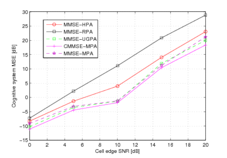
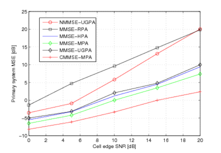
Refer to caption — Fig. 1: Cognitive system MSE vs cell edge SNR

Figure (2) illustrates the contamination and its impact on MSE performance of the PU. It can be clearly noted that the CU existence has a powerful impact on the estimation process. The modified MMSE estimator with MPA has a superior performance in the rejection of the interference especially at SNR, due to its capability of limiting the interference to certain value. On other hand, using RPA at the CBS has a very harmful impact on the estimation at PBS since it does not take into the account the spatial separability between the CUs and the PU. The user grouping PA and heuristic PA show less impact on PU in comparison with RPA, which motivates their usefulness due their simple implementation.

VI Conclusion

In this paper, we discussed the impact of pilot contamination during channel estimation and its influence on primary and cognitive systems. We presented and studied the performance of different MMSE techniques. We proposed modified estimation and pilot allocation techniques to tackle the primary-cognitive hierarchy. They enabled enhanced estimation by reducing the overlap in the interfering subspaces and boosting the separation in the signals through allocating the same pilot to CUs that has distinct spatial characteristics from PU. Moreover, different pilot allocation techniques are proposed to enhance the estimation and to reduce the impact of contamination on the two systems. The performance of introduced algorithms was investigated and compared to current state of the art techniques. From the simulation results, it can be concluded that the proposed MMSE estimation techniques combined with pilot allocations provide considerable gains over the traditional techniques.

acknowledgment

This work was supported by the National Research Fund (FNR) of Luxembourg under the AFR grant (reference 4919957) for the project Smart Resource Allocation Techniques for Satellite Cognitive Radio.

References

[1] A. Goldsmith, S. A. Jafar, I. Maric, and S. Srinivasa, “Breaking spectrum gridlock with cognitive radios: An information theoretic perspective,” IEEE, vol. 97, no. 5, pp. 894 - 914, May 2009.
[2] S. Haykin, “Cognitive Radio: Brain-Empowered Wireless Communications,” IEEE Journal on Selected Areas in Communications, vol. 23, pp. 201-22, Feb. 2005.
[3] S.H. Song and K. B. Lataief,“Prior Zero-Forcing for Relaying Primary Signals in Cognitive Network,” IEEE Global Conference in Telecommunications (Globecom), December, 2011.
[4] K.-J. Lee and I. Lee “MMSE Based Block Diagonalization for Cognitive Radio MIMO Broadcast Channels,” IEEE Transactions on Wireless Communications, vol. 10, no. 10, pp. 3139 - 3144, October 2011.
[5] S. K. Sharma, S. Chatzinotas and B. Ottersten,“Spectrum Sensing in Dual Polarized Fading Channels for Cognitive SatComs,” IEEE Global conference on Telecommunications(Globecom), December 2012.
[6] J. Jose, A. Ashikhmin, T. L. Marzetta and S. Vishwanath, “Pilot Contamination and Precoding in Multi-Cell TDD Systems,” IEEE Transactions on Wireless Communications, vol. 10, no. 8, pp. 2640 - 2651, Aug. 2011.
[7] N. Krishnan, R. D. Yates, and N. B. Mandayam, “Cellular Systems with Many Antennas: Large System Analysis under Pilot Contamination,” Allerton Conference on Communications, Computing and Control, October, 2012.
[8] M. Alodeh, S. Chatzinotas and B. Ottersten,“Spatial DCT-Based Least Square Estimation in Multi-antenna Multi-cell Interference Channels,” to appear in IEEE International Conference on Communications (ICC), 2014.
[9] M. Alodeh, S. Chatzinotas and B. Ottersten,“Spatial DCT-Based Channel Estimation in Multi-Antenna Multi-Cell Interference Channels,” submitted to IEEE Transactions on Signal Processing, available on Arxiv.
[10] H. Yin, D. Gesbert, M. Filippou and Y. Liu, “A Coordinated Approach to Channel Estimation in Large-scale Multiple-antenna Systems,” IEEE Journal in selected Areas in Communications, vol. 31 , no. 2, pp. 264 - 273, February 2013.
[11] J. Nam, J.-Y. Ahn, and G. Caire, “Joint Spatial division and Multiplexing-The large Scale Array Regime,” IEEE Transaction on Information Theory, vol. 51, no. 5 , pp. 6441 - 6463, October 2013.
[12] A. Adhikary, and G. Caire, “Joint Spatial Division and Multiplexing: Opprtunistic Beamforming and User Grouping,”Available on Arxiv.
[13] A. Scherb and K. Kammeyer, “Bayesian channel estimation for doubly correlated MIMO systems,” IEEE Workshop on Smart Antennas (WSA), 2007.
[14] P. Zetterberg and B. Ottersten, “The spectrum efficiency of a base station antenna array for spatially selective transmission,” IEEE Transactions on Vehicular Technology, vol. 44, no. 3, pp. 57-69, Aug. 1995.