Random Coulomb antiferromagnets:
from diluted spin liquids to Euclidean random matrices
Abstract
We study a disordered classical Heisenberg magnet with uniformly antiferromagnetic interactions which are frustrated on account of their long-range Coulomb form, i.e. in and in . This arises naturally as the limit of the emergent interactions between vacancy-induced degrees of freedom in a class of diluted Coulomb spin liquids (including the classical Heisenberg antiferromagnets on checkerboard, SCGO and pyrochlore lattices) and presents a novel variant of a disordered long-range spin Hamiltonian. Using detailed analytical and numerical studies we establish that this model exhibits a very broad paramagnetic regime that extends to very large values of in both and . In , using the lattice-Green function based finite-size regularization of the Coulomb potential (which corresponds naturally to the underlying low-temperature limit of the emergent interactions between orphan-spins), we only find evidence that freezing into a glassy state occurs in the limit of strong coupling, , while no such transition seems to exist at all in . We also demonstrate the presence and importance of screening for such a magnet. We analyse the spectrum of the Euclidean random matrices describing a Gaussian version of this problem, and identify a corresponding quantum mechanical scattering problem.
pacs
xxI INTRODUCTION
The appearance of novel magnetic phases[1, 2, 3] generally contains as one ingredient the ability of the system to avoid conventional (semi-)classical ordering. In this connection, the role of several factors has been extensively explored. These include low dimensionality and the resulting enhancement in the effects of quantum and entropic fluctuations, geometrical frustration, whereby the leading antiferromagnetic interactions compete with each other on lattices such as the kagome and pyrochlore lattice, and the presence of quenched disorder, which disrupts any residual tendency to conventional long-range order. Each of these has given rise to research efforts spanning decades of work.
Here, we study a model with a new combination of some of these ingredients. The focus of our study is a disordered classical Heisenberg magnet with antiferromagnetic interactions which are frustrated on account of their long-range Coulomb form at long-distances, i.e. in (where is a length-scale of order the system-size) and in . This Coulomb form of the Heisenberg couplings arises naturally as the limit of the emergent entropic exchange interactions [4] between vacancy-induced “orphan-spin” degrees of freedom [5, 6, 7, 8] in diluted Coulomb spin liquids, and presents a novel variant of a disordered long-range spin Hamiltonian with connections to Euclidean random matrices. The coupling constant is determined in any given system by the microscopic details of the underlying Coulomb-spin liquid, while the spin degrees of freedom in the model we study are related to the physical orphan-spins of the underlying diluted magnet. Our focus here is on studying the range of behaviours possible in the limit by mapping out the phase diagram of our Coulomb antiferomagnet as a function of . Frustration arises naturally in the model under consideration, as any triplet of spins are mutually coupled antiferromagnetically but without the randomness in sign of, say, the Sherrington-Kirkpatrick model [9]. Also, unlike the latter case, the interactions are long-ranged but not independent of distance.
Our motivations for studying it include having been led to this model in a previous investigation [10] of diluted frustrated magnets exhibiting a Coulomb spin liquid at low temperature. The model is in this sense natural, appearing as the zero-temperature limit of a disordered frustrated magnet. The corresponding experiments are on the material known as SCGO, which triggered the interest in what we now call highly frustated magnetism in the late 80s [11]. Its behaviour at very low temperatures is still not very well understood, e.g. the observed glassiness even at very low impurity densities [12, 13], which appears to involve only the freezing of a fraction of its degrees of freedom. We will return to this point in Sec. VII.2. While exhibiting a classical Coulomb spin liquid regime, the disorder in this system leads to the emergence of new, fractionalized, degrees of freedom, the so-called Orphans [5, 6], which interact via an effective entropic long range interaction mediated by their host spin liquid [4].
We believe that as such, it can be of interest as a generic instance of the interplay of strong interactions and disorder in magnetism. In particular, it develops the strand of thought of how disorder in a topological system characterised by an emergent gauge field can nucleate gauge-charged defects, with the pristine bulk mediating an effective interaction between them. Long-range Coulomb interactions like the one studied here are then as natural as the algebraically decaying RKKY interactions in metallic spin glasses.
Our central results are the following. First we use the results of previous work[4], to work out in detail the key features of this limit, and demonstrate that this limit is characterized by a single coupling constant , which is, in principle, determined by the geometry of the underlying spin-liquid. Second, our extensive Monte Carlo simulations for reveal no sign of any freezing or ordering transition up to very large coupling strengths. At the same time, within a self-consistent Gaussian approximation, we find that there does appear such a transition at infinite coupling in but not in . This transition is very tenuous, in that it is replaced by a more conventional ordering transition in a finite system depending on the choice of how to regularize this long-range interaction in a finite lattice: the finite-size lattice regularization that is most natural from the point of view of the limit of the underlying diluted magnet gives rise to freezing into a glassy state at , while other regularizations replace this glassy state by a conventional ordering pattern. The Coulomb antiferromagnet therefore remains highly susceptible to perturbations, just like many other frustrated magnets [1].
We also study the spectrum of the interaction matrix of this random Coulomb antiferromagnet, which provides an instance of an Euclidean random matrix [14, 15], in that its entries are obtained as a distance function between randomly chosen location vectors. We find two qualitatively distinct regimes. On one hand, at low energies in the low-density limit, eigenfunctions are localised, with the lowest energy states as pairs of neighbouring spins the probability distribution of which we compute. Beyond this extreme low-density limit, more complex lattice animals appear in this regime. On the other hand, at high energies, the modes correspond to long-wavelength charge density variations with superextensive energy. In between, we find no clear signature of a well-defined mobility edge in this Coulomb system.
Another interesting aspect of the uniformly antiferromagnetic interactions is that they permit a variant of screening to appear in this Coulomb magnet, which has no correspondence with other long-range magnets such as the Sherrington-Kirkpatrick model. Our analysis of this screening further leads us to an identification of the correlations of the random Coulomb antiferromagnet with the properties of the zero-energy eigenstate of a quantum particle in a box with randomly placed scatterers.
Returning to experiments, we note that the uniform magnetic susceptibility of SCGO will of course be dominated by the Curie tail () produced by these orphan spins at low temperature. Both in and , the full susceptibility, when vacancies are placed at random, is that of independent orphans to a good approximation despite the long-ranged interaction present between them. This persists down to the lowest temperatures not only because of the screening of the interactions at finite physical temperature, and because the size of the Coulomb coupling derived from the entropic interaction is comparatively weak, but also because the physical orphan spins are related to the degrees of freedom in the Coulomb antiferromagnet via a sublattice-dependent staggering transformation, so that the uniform susceptibility of the physical orphan-spins corresponds to the staggered susceptibility of the degrees of freedom of our Coulomb antiferromagnet, and therefore remains largely unaffected by the fact that the total (vector) gauge charge of our Coulomb antiferromagnet vanishes.
The remainder of this paper is structured as follows. In Section II, we first provide a self-contained review of earlier work on vacancy-induced effective spins in a class of classical antiferromagnets on lattices consisting of “corner sharing units”, and then build on this to provide a careful derivation of the limit of the emergent entropic interactions between orphan spins and use this to define our model Coulomb antiferromagnet. After outlining our analytical and numerical approaches in Sec. III, we present the results obtained in and (Sec. IV). Sec. V contains the analysis of the problem in terms of a Euclidean random matrix while the role of screening and the connection to a scattering problem are discussed in Sec. VI. We conclude with a discussion of these results, and relegate sundry details (such as dicussions of the fully occupied lattice and the ordered state seeded by a certain finite-lattice regularization of the two-dimensional Coulomb interaction) to Appendices.
II The random Coulomb antiferromagnetic Hamiltonian
We thus study a classical Heisenberg model
| (1) |
where takes on a Coulomb form,
| (2) | |||||
| (3) |
This form with larger than any has the property that the interactions are uniformly antiferromagnetic as well as long-ranged.
We need to supplement this by defining the degrees of freedom, unit vectors , appearing in Eq. 1. We concentrate on the case where their locations, denoted by are chosen randomly on a square (cubic) lattice in (), at a dimensionless density of spins per lattice site.
For long-range interactions like this Coulomb interaction, choices about boundary conditions or ensemble constraints can be considerably less innocuous than for short-range systems. In order to illustrate this, and to make natural choices for these items, as well as for motivation of our study, we discuss the derivation of a random Coulomb antiferromagnet as an effective Hamiltonian of a diluted Coulomb spin liquid next.
II.1 Orphan spins and their interactions in diluted Heisenberg antiferromagnets

We thus begin by providing a self-contained review of earlier work on vacancy-induced effective spins in a class of classical frustrated antiferromagnets on lattices consisting of “corner sharing units”. The centers of these in turn define a so-called premedial lattice, which is bipartite in practically all instances of popularly studied classical Heisenberg spin liquids [8]. A simple model of nearest neighbour antiferromagnetically interacting spins on such lattices can be written as
| (4) |
where the summation in the alternate form of the Hamiltonian is carried over the corner sharing simplices , which might be tetrahedra, as e.g., in a pyrochlore lattice, triangles in a Kagome lattice, or a combination of both as in the case of SCGO, and the spins of the frustrated magnet are now labeled by , the links of the bipartite pre-medial graph (whose sites correspond to the centers of the simplices of the original lattice, and links correspond to sites of the original lattice). When written in this form, it is clear that ground-states are characterized by the constraints:
| (5) |
These local constraints lead to an effective description in terms of a theory of emergent electric fields that obey a Gauss law. To see this, we define electric fields on links , where is a spatial unit vector that points from the - to the -sublattice of the premedial lattice end of this link. The ground-state condition then translates to the statement that the lattice-divergence of this electric field vanishes at each site for each . The key idea of this effective description is that the coarse-grained (entropic) free energy density depends quadratically on the local electric field, and deviations from the vanishing divergence condition amount to the appearance of vector Coulomb charges [4]. These emergent gauge charges are defined for each lattice point of the bipartite premedial lattice:
| (6) |
and the staggering factor, if is an -sublattice site of the premedial graph and otherwise. Since each microscopic spin contributes with opposite signs to the vector charge on two neighbouring simplices, the total gauge charge of a system without boundaries must vanish in every configuration of the system
| (7) |
This very natural condition–akin to the charge-neutrality of the full universe, and in our case unavoidable due to the microscopic origin of the emergent gauge charge – will be explicitly imposed in our Monte Carlo simulations of the system.
The mapping of the pure system to an emerging gauge field theory at low temperatures makes clear that generalized “vector charges”, , are generated thermally as a consequence of the violation of the ground state constraints. The constraint Eq. 5 is also unavoidably violated in the presence of non-magnetic impurities (Fig. 1) whenever all but one spin of a given simplex are substituted for by vacancies (simplices containing at least two spins can in general satisfy the zero total spin condition and such simplices do not host a vector charge in the limit). Indeed, when all spins but one in a simplex are replaced by vacancies, the result is a paramagnetic Curie-like response [6, 10, 4], which dominates the susceptibility response at low temperatures. The lone spins on these defective simplices, which serve as the epicenter of this paramagnetic response, were baptized Orphans (Ref. 5) in the first studies of this effect.
The field theory developed in Refs. 10, 4 extends the self consistent gaussian approximation (SCGA) [16], a theory successful in describing low temperature correlations on the undiluted systems, to incorporate the effects of dilution and study the physics of these orphan spins at non-zero temperature in a manner that treats entropic effects on an equal footing with energetic considerations. In its original form the SCGA replaces the hard constraint on the spins norm, , by the relaxed soft spin condition on their thermal average . The key insight of Refs. 10, 4, that led to the detailed analytical understanding summarized below, was the following: While it is sufficient to treat in this self-consistent Gaussian manner all spins other than the lone orphan spin in a simplex in which all but one spin has been replaced by vacancies, this is much too crude an approximation for the orphan-spin itself, which must be treated without approximation as a hard-spin obeying . Remarkably, the resulting hybrid field theory continues to be analytically tractable when the number of orphan spins is small[10, 4]. With just one orphan present in a sample with an external magnetic field of strength along the axis, the theory predicts that this orphan spin sees a magnetic field , with the other half of the external field screened out by the coupling to the bulk spin-liquid. The resulting polarization of the orphan serves as a source for an oscillating texture that spreads through the bulk. The net spin carried by the texture cancels half the spin polarization of the orphan-spin, resulting in an impurity susceptibility corresponding to a classical spin . With more than one orphan present, the spin-textures seeded by each orphan mediate an effective entropic interaction between each pair of orphan spins.
The effective action for a pair of orphans is predicted in this manner to have the form
| (8) |
where are unit-vectors corresponding to the directions of the orphan-spins in a given configuration. The exchange coupling has a particularly simple form in the large separation limit
| (9) |
which involves only “charge-charge” correlations calculated in the pure system:
| (10) |
The denominator of Eq. (9), behaves at low temperatures as from equipartition.
For orphans in , one finds:
| (11) |
with an entropic screening length separating two regimes for . For a logarithmic one, ; and for a screened regime, . Analogously in ,
| (12) |
the entropic screening length separates two regimes, algebraic and screened .
In the physical system, at any nonzero temperature, this is thus a ‘short-ranged’ interaction on account of the finite screening length which, however, diverges as . In this article, we are interested in the limit of , where the interaction takes on the novel – for magnetic systems – long-range Coulomb form.
II.2 Model Hamiltonian
In the limit of , we are thus led by these considerations to Coulomb interactions between the vector orphan spins, which we here study in detail. For simplicity, we consider unit-vector spins at random locations in a periodic hypercubic lattice of linear size with occupancy probability , corresponding to an underlying spin liquid on the checkerboard and “octochlore” lattices of corner-sharing units involving spins in dimension.
In what follows, we will get rid of the sublattice factors that affect the sign of the effective interaction by inverting all unit-vectors placed on the sublattice. In other words, we identify with , where is the orphan spin on the simplex labeled by in the underlying diluted frustrated magnet.
This gives us a “random Coulomb antiferromagnet” in which unit-vector spins interact with an exchange coupling that is always antiferromagnetic but of a long-range Coulomb form at large distances. For a classical system, this transformation is innocuous, but note that natural observables cease to be so under this mapping – e.g. the orphan spin contribution to the uniform susceptibility of the underlying diluted magnet is now given by the staggered susceptibility of our Coulomb antiferromagnet.
As is usual for entropic interactions in the limit of , the strength of their coupling, , is fixed by the microscopics of the model from which they have emerged. In this work, we are interested in exploring the generic behaviour of such models – in particular, identify possible phases – and thus allow the coupling to be variable. For completeness, we mention that for the checkerboard lattice.
This therefore leads to the form of at the beginning of this section, Eq. 1. To make Eq. 2 dimensionally unambiguous we write:
with conveniently set to a value of order the system size so that always. In the above language, with sublattice factors absorbed into the definitions of , the zero gauge-charge constraint imposed by the microscopic origin of this effective model now translates to the constraint that in every allowed configuration of our Coulomb antiferromagnet. This constraint in fact can also be imposed by adding an infinitely strong interaction acting equally between all spins. This equivalence renders the detailed choice of immaterial.
We note an interesting scale-invariance of this model in the limit of small densities of spins. This scale invariance is inherited from that of the logarithmic function under scaling transformations: , together with net charge neutrality Eq. (7):
| (13) |
implies that the extra term gives a temperature-independent contribution to the action determined by . The partition function thus only picks up a constant factor:
| (14) |
It also means that, rather unusually, in the continuum limit the partition function is a scaling function depending on the randomly chosen orphan locations only scaled by their mean separation. Lattice discretisation effects at finite break this equivalence. The scaling transformation for the model in three dimensions gives , what implies for the partition function a rescaling of :
| (15) |
For Coulomb interactions in a finite-size system, various choices of the interaction yield the same large-distance form in the limit . The most natural form from the point of view of the effective field theory predictions for emergent interactions between orphan spins is the Fourier transform of the inverse of the lattice Laplacian, :
| (16) |
This we call the lattice Green function (LGF), and our most detailed studies are carried out with this form of the interaction.
Alternatively, one can work directly with the Coulomb form, e.g. for :
| (17) |
with .

This form agrees with the LGF interactions at short distances (see Fig. 2).
The issue of how to impose the boundary conditions, and therefore how to compute , turns out to make much difference on the results for a finite system, as we shall see. The choices of either
| (18) |
with or
| (19) |
result in different behavior for the system, which will be explained in more detail in the results section. We refer to these choices as periodised, and smoothed, logarithms, respectively. The latter is very close to the LGF, while the former maintains a finite difference to it at the periodic boundary, where it is not differentiable for any (Fig. 2). It is easily seen why this finite difference is independent of , if one compares the smoothed log to the periodized Log, approximatelly equivalent to comparing the LGF with the Log. Looking, e.g., at the midpoint of one edge (, ) one finds:
| (20) |
where the subindex emphasizes that we are looking at the respective forms of the interactions in a finite system of size .
Note, again, that adding a constant to the interaction (in ), e.g., by changing the denominator of Eq. (17), leaves the interaction unchanged due to the global charge neutrality constraint.
III Methods
The analysis of spin systems with the potential for glassy phases is a delicate endeavour as equilibration of large systems is elusive. Existence and determination of a transition temperature is usually a controversial issue[17, 18]. Since our system has long ranged interactions, boundary effects can cause yet more trouble. This is why we combine analytical with numerical methods, as well as mappings to other problems which have received attention in a different context previously.
Numerically, we study the behaviour of this model through Monte Carlo (MC) simulations, and analytically in the self-consistent Gaussian (“large-m”, also denoted in the following as LM approach [19, 20, 21]) approximation, where the parameter mimics an inverse temperature. Our MC simulations directly impose the constraint, Eq. (7). For that we initialize the system in a random configuration of vanishing total spin, and the update movements on the system consist of selecting an arbitrary pair of spins, and rotating them around the axis determined by their vectorial sum. A MC simulation of the same system with strictly positive interactions, without this constraint on the total spin has been also investigated, and the conclusion is that while the relaxation time increases, the system still prefers to stay close to the manifold of vanishing total spin.
The LM approach consists of considering spins with components and letting . This is formally equivalent to the soft spin approximation and it only gives in principle information about the infinite number of components limit, but this can be understood as the 1st term in an expansion of the model. It has been very successful in the analytical study of correlations in highly frustrated spin systems [16], being able to reproduce the main features of the on-going phenomena, such as existence of long range dipolar correlations at , characterized by the presence of “pinch points” in the structure factor [22].
The LM approach allows an analysis of the system both at finite coupling strengths , and at . The study of glassiness with this approach has been already undertaken in a variety of models [21, 23], and we will be following a similar methodology. Correlations are computed through the matrix:
| (21) |
and are given by:
| (22) |
These can be computed once the Lagrange multipliers, , are determined through the set of nonlinear equations:
| (23) |
For comparison between LM and MC, we scale observables and couplings with so that their small-coupling (“high-temperature”) forms agree.
The point is treated within the LM approach by determining the (unique [19]) ground state through a local field quench algorithm [24]. This algorithm is based on the fact that if the number of spin components, , is large enough (larger than [19]), then a system of spins with components is effectively equivalent to the corresponding system in the limit . The algorithm then consists of taking a system of spins with components initially randomly oriented, and then iteratively aligning each spin with its local field. This procedure is expected to converge to the unique ground state, from which all the quantities of interest can be computed.
A fundamental quantity at within the LM approach is the number of zero eigenvalues, , of the matrix ; it can be shown[19] that the ground state spin vectors span an dimensional space. This quantity should scale with the number of particles in the system as . Furthermore, as was shown in Ref. 21, the same exponent controls the scaling of the spin glass susceptibility for the ground state configuration: .
The main quantity of interest in our study will be the spin glass susceptibility (square brackets here and throughout indicate the disorder average),
| (24) |
obtained in the MC simulations through the overlap tensor [3]:
| (25) |
where greek indices refer to the spin components, while the indices refer to two independent replicas of a disorder realisation. This might be interpreted as the overlap of a spin configuration with itself after an infinitely long time. Since the onset of glassiness can be also understood as a divergence of the equilibration time, the nonvanishing of this order parameter signalizes the transition.
The spin glass susceptibility in terms of this tensor is:
| (26) |
We follow the usual practice to determine the spin glass transition by computing a finite system correlation length associated to the susceptibility above. The Ornstein-Zernike form for correlations gives:
| (27) |
and near the transition, the finite size scaling prediction is expected to be:
| (28) |
while the susceptibility should follow:
| (29) |


Notice that these scaling relations only hold if there exists a crossing of finite size correlation length curves for different system sizes at an unique finite coupling strength value. The absence of such a crossing at a finite indicates the absence of a phase transition. Nonetheless a phase transition at cannot thus be ruled out and the LM approach allows an analysis in this situation. The scaling relations predicted to hold in this case () are:
| (30) |
The exponent here is the one previously introduced for the scaling of the number of zero eigenvalues of the matrix with the number of particles in the system.
IV Results
IV.1 Two dimensions


The two approaches (MC and LM) yield a broadly consistent picture for each of the interactions studied. We conduct an analysis of a possible freezing transition in the model by measuring the spin glass susceptibility and trying to identify the transition through a finite size scaling of its associated correlation length. Other observables such as the specific heat or the uniform susceptibility were also studied, though these do not indicate any of the conventional orderings.
The results from MC simulations and LM calculations are shown on Fig. 3 for the system with LGF as interaction for a fixed density of particles. In each case the number of disorder realisations simulated was .
Globally, correlations are stronger for the MC simulations on Heisenberg spins compared to the LM results. This is in keeping with the general lore that a lower number of spin components is conducive to spin freezing, as is well known from the comparison of Ising and Heisenberg spins.
In the broad range of coupling strengths considered by our analysis, no unique crossing for the different system sizes of the correlation length curves can be identified.
The LM analysis at yields the exponent as indicated in Fig. 4. This seems to have the same value, for both the LGF and Log interactions.
The exponent value is used as input, together with the assumption that for the LGF, in attempting a scaling collapse of the LM data. The exponent was determined by a fitting procedure with the scaling relation, Eq. (30), only using data for the correlation length. The resulting scaling collapse is shown on the inset of the lower panel of Fig. 3, where is obtained. Finally, we use all these exponents on the predicted scaling relation for the susceptibility (the result is shown on the inset of the upper panel of Fig. 3). The available data from the LM calculations indicates therefore a freezing transition at for the diluted model with LGF as interaction in two dimensions.


The Log interaction turns out leads to a dramatically differing behaviour! This is a surprising result, as the interactions only differ appreciably at large distances (Fig. 2). Fig. 5 shows the results for the observables of interest as obtained from MC simulations and LM calculations, respectively. Here again we fix the density of particles , and consider disorder realisations. A clear crossing of the correlation length curves for different system sizes occurs and scaling collapses of the data are possible, which are shown together with the corresponding critical exponents as insets.


To study more closely this effect, we consider the pair correlations as a function of the relative coordinates of the pairs, averaged over disorder realisations (Fig. 6). The profile is isotropic for the LGF with only the 1st few nearest neighbors significantly antiferromagnetically correlated. On the other hand, the Log interaction yields strongly anisotropic behavior (the interaction itself is anisotropic) and this seems to be responsible for what we see as a “glassy phase transition” emerging from the “splaying out” of the susceptibility curves. The absence of glassiness is explained in more detail on Appendix A, where we expose how the pair correlation profile helps us in defining an appropriate susceptibility for the case at hand, which is shown to diverge in the thermodynamic limit. It turns out that this reflects not the existence of true glassiness but a transition closer to conventional ordering. Note that the gross features of the correlations (Fig. 6 lower panel) follow if one frustrates the pairs at the kink (Fig. 2) of the Log interaction, which form a frame at half the system size. The set of points which in turn are on the “frames” of points on the first frame yield the cross shaped set of ferromagnetically correlated sites centred on the origin.
Note that such finite-size differences appear to be absent in previous studies in [25]; they appear to be a consequence of the anisotropic nature of our periodised Log interaction with its non-analytic minimum at maximum separation. By contrast, the “smoothed Log” (Fig. 2) that also respects the periodic boundary conditions essentially reproduces the LGF interaction results.
IV.1.1 The fully covered square lattice
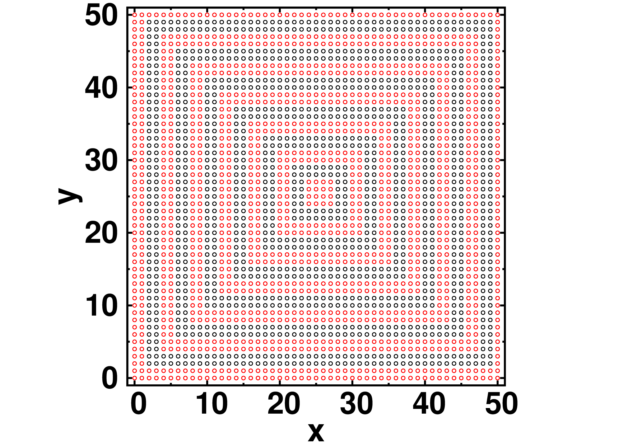
For completeness, we have also analysed the situation for a fully occupied lattice. In this case we observe that the LGF interaction leads to conventional (Néel) antiferromagnetic order, while the Log leads to a “striped” phase. This can be understood from a theorem in Ref. 26 which states that the ground state of the system is determined by the minimum of the Fourier transform of the interaction. This is explained in more detail on Appendix B.
IV.2 Three dimensions
We analyse the diluted cubic lattice considering a density of particles , and again considering the model Hamiltonian of Eq. (1), with interactions now restricted to be the LGF as given by Eq. (16). Both Monte Carlo simulations and LM calculations cover several system sizes with distinct disorder realisations each. The main focus is on the possibility of a glassy phase and the spin glass susceptibility and corresponding correlation length are computed. Our prior discussion of the finite size scaling relations still holds, and one determines the transition as an unique crossing of the finite size correlation length curves. Instead of this we observe (Fig. 7) a trend for the crossings to shift towards larger values of as the system size increases, similar to the situation in two dimensions.


No good scaling collapse was obtained. A freezing transition in this system at a finite coupling strength therefore appears unlikely, though a more careful finite size scaling analysis of the crossings is necessary to give a definitive answer.
A LM study at reveals that the exponent for the scaling of zero eigenvalues of the matrix with system size yields , in agreement with the prediction in 3 dimensions for a short ranged interacting system [21]. Using of this exponent and the scaling relations at does not lead to a good scaling collapse of our LM data, reinforcing the conclusion that this system does not present any freezing transition at .
The pair correlations exhibit the same sort of behavior as in the 2d case: only the 1st few nearest neighbors tend to be strongly antiferromagnetically correlated, but no correlations develop at large distances as the coupling strength is increased, and the system remains paramagnetic.

V Spectral properties
The transition can be considered from the point of view of the interaction matrix (16) and (17), as an example of euclidean random matrix (ERM): [14] unlike the traditional random matrices, where different entries of the matrix are uncorrelated, ERM’s are defined by a function of the distance between two points , where the randomness in the entries is induced by the randomness of the underlying point pattern . These random matrices have been studied for certain classes of functions [15], and some classical results are available. Our degree of understanding of this subject is not comparable to that of the classical (e.g. GOE,GUE, Wishart) ensembles [27] with most results coming from exact diagonalisation and approximations [15, 14, 28].
Unfortunately due to the long-range nature of the -interaction, many of the methods to analyse the spectral properties presented in Ref. 15 do not apply directly to our case. However, a phenomenological picture of the low- and high-lying eigenstates of the matrix can be established transparently.

Let us start from the large positive eigenvalues. Since is constant in sign, the Frobenius-Perron theorem states that a highest eigenvector is nodeless. To a reasonable approximation, it is fully delocalised,
| (31) |
The associated eigenvalue is
| (32) |
with an inverse participation ratio of .
The second-to-highest eigenvalue is also associated to a delocalised eigenvector, which is now a wave with wavelength . At these length scales the randomness of the point process plays little role. A finite fraction (possibly all) of the eigenstates containing the largest eigenvalues are delocalised, they correspond to long-wavelength charge-density variations. The average spectral density (DOS) of the LGF (16) interaction matrices is shown on top panels of Figs. 10 and 11, in the limits of high () and low density (‘continuum limit’, ), respectively.
Guided by the numerics, we see that the eigenvectors corresponding to the most negative eigenvalues are localised eigenvectors: most of the weight is concentrated on spins. This leads us to consider isolated percolation animals.
The simplest (and, for small , the most abundant) of these is the dimer. A well-isolated dimer supports two eigenvalues: an antisymmetric and a symmetric one. The antisymmetric one,
| (33) |
corresponds to the smallest eigenvalue. In fact, since the closest pair is located one lattice spacing away and the lowest eigenvalue is
| (34) |
At fixed density, , the lowest eigenvalue depends logarithmically on the system size.
For a well isolated dimer, say at distance from the closest spin, the effect of neglecting the rest of the spins appears as a correction .


We now consider how big this isolation distance is. By the usual arguments of percolation theory, one can estimate the expected number of isolated dimers as
| (35) |
where we have approximated the number of lattice sites in a circle of size with . Therefore the most isolated dimer (the solution of the equation ) is surrounded by an empty area of size
| (36) |
Note the extremely slow dependence .
Inserting and , which is about the largest sizes considered in our numerics, , which can hardly be called isolated.
The isolation effect would be much more pronounced for , for which . Otherwise, one needs to consider the ground states of more complicated lattice animals, like trimers, snakes, squares etc. As an example, a ground state eigenvectors for one disorder realisation is shown on Fig. 9.
This problem becomes quickly analytically prohibitive. However the fact that the ground state is localised on some lattice animal appears robust: on the graphs we consider, the smallest eigenvalue is and the IPR is .


With the lower end of the spectrum localised and the high-end delocalised, it is a natural question whether there exists a mobility edge separating the two limits. In order to study the transition we have looked at the inverse participation ratio as a function of the eigenvalue :
| (37) |
where and are eigenvalues and normalized eigenvectors of respectively. We consider the average and fluctuations . [29] A mobility edge would be signaled by the divergence of the fluctuations of at a certain . Numerical diagonalization of does not indicate such a transition: the two limits appear to be separated by a crossover. The bottom panels on Figs. 10 and 11 show, respectively for a high and low density of particles, the average , while the insets display the fluctuations of . The spectral properties of the LGF in turn out to be very similar to the case (not shown).
A detailed study of this ERM ensemble would be desirable and is left for future work.
VI Pair correlations and screening
VI.1 Analytical theory of screening
Away from the limit of the microscopic model, excitations of the non-orphan tetrahedra out of their momentless state carry gauge charge, which leads to a variant of Debye screening, with the special feature that the gaplessness of the charge excitations leads to a somewhat unusual temperature dependence of the screening length [30].
In addition to this, even in the limit studied here, we encounter an additional type of screening. This occurs on account of the long-range uniformly antiferromagnetic Coulomb interaction between the orphan spins, whose existence is the distinguishing property of the random Coulomb antiferromagnet. It again exhibits a Debye form, although distinct from the setting of mobile charges in which Debye screening is normally considered, as here it is the (continuous) flavour of the charges – the orientation of the orphan spin whose orientation is free but whose location is fixed – which is the dynamical degree of freedom.
This can be seen directly in a weak-coupling expansion, which in Coulomb systems has a vanishing radius of convergence in the thermodynamic limit, as is easily verified in our simulations, Fig. 12.

To elucidate the role of screening, we compute the disorder averaged correlator between two spins at and . Consider the Hamiltonian
| (38) |
where are given by either the Log or the LGF and we will eventually set . The correlation function between two spins, for fixed disorder is:
| (39) |
As it is not the hard spin constraint which is central to the physics of screening, we substitute it with something more manageable (analogously to the LM method, but without imposing self-consistency). Representing the delta function with a Gaussian term
| (40) |
(with a factor of to guarantee that ). Thus
| (41) |
where we use a matrix notation . For simplicity we will not write the term, which only affects the result for the self-correlation (it will return to be important when we discuss the LM approximation again later). The correlation function between and depends also on the positions of all the other points so it should be written as .
This Gaussian approximation is equivalent to the resummation of a set of diagrams in which there are no internal loops, dubbed “chain diagrams.” This approximation is justified in the limit of small , in which spins are rarely polarized along some direction and the hard-spin constraint is not so important.
This result holds for each disorder realization. We now take the average over realizations (leaving the question of whether this is representative of the distribution or not for later) keeping fixed the position of the two spins . For doing this, it is convenient to go back to the geometric expansions and define
| (42) |
where are the locations of the other spins and . We have relaxed the constraint that points be located on a square lattice, which is immaterial in our high temperature, low-dilution expansion.
Unfortunately it is difficult to see what the distribution of induced by the random positions is, but we can expand the Gaussian result in powers of and do the average term by term.
We get
| (43) | |||||
Now, term by term we obtain objects like
| (44) | |||||
where is the density of points. Fourier transforming,
| (45) | |||||
| (46) |
The geometric series obtained thus for yields
| (47) |
Now, for both Log and the LGF, ( is a constant of ) [31] so that at small we have approximately
| (48) |
This leads to
| (49) |
which exhibits a screening length
| (50) |
As both and are this shows (not surprisingly) that the screening length is proportional to the .

Note that in this approximation, for the correlation function , which is not physical for unit length spins. This is an artefact resulting from substituting the hard spin constraint with a quadratic confining potential. Therefore this approximation is internally consistent only for , where it predicts an exponential damping of the correlations but we note that the large anticorrelations at short distance due to strongly coupled spins close to one another put these into a state with vanishing total spin, which – physically correctly – screens their joint field at larger distances.
VI.2 A random scattering picture
The final question we address concerns the fluctuations of the random quantity (41) and whether these may signal any phase transition even when the mean does not. To gain some insight into this, we develop an analogy with wave propagation in disordered media, which suggests that no transition exists. The basic observation is that the interaction is simply related to the inverse of the Laplacian, the propagator of a free particle on the lattice:
Considering that
| (51) |
properly regularized (particularly important is the condition that ), we can rewrite the expression (41) as
| (52) |
where and
| (53) |
is a random potential. This can be established by expanding in powers of .
Thus is (proportional to) the propagator for a wave in a two-dimensional box with randomly placed point-like scatterers [32, 33], at energy .
The precise form of the mapping is the following: the correlation function
| (54) |
is the amplitude of a signal sent from the scatterer to the scatterer , considering all order processes bouncing over all the scatterers. In case the direct path from to needs to be neglected. This is a form of renormalization of the scattering problem which is always necessary in the point-like (or -wave) scattering limit [34].
Once the renormalization procedure is done, the problem we are left with corresponds to the propagation of a scalar wave, damped by a scattering section for every typical realization of disorder. Without repeating the classical treatment of this phenomenon we can say that the signals (spin-spin correlations) must be screened for any , the screening length (measured in units of ) being a decreasing function of . Even if not precisely of the form (50) for small-, it seems to diverge like .
This is valid both for the coherent field and the incoherent field , although the scattering sections (and hence the damping/correlation lengths) might have different values. This analogy makes us realize that in this approximation there is no transition irrespective of the value of or , and this is consistent with numerical results.
This analogy extends also to the LM limit. Considering a small- series expansion for the spin correlation function:
| (55) |
(recall that in LM is scaled by a factor , hence the factor of 3 of the previous paragraphs is absent here) where the extra factors of need to be chosen in such a way that
| (56) |
is then proportional to the propagator
| (57) |
where is the diagonal matrix with diagonal entries , and
| (58) |
where the renormalized value is intended.
This is a scattering problem over point-like scatterers, where now each scatterer has different scattering amplitude. This modification should not change the physical analogy of the problem. This is again a scattering problem of a scalar wave over point-like scatterers. The propagation of the wave is attenuated over distance in the usual exponential fashion. Therefore, if a phase transition exists, it is not mirrored in the divergence of the correlation length. Conversely, as this treatment is closely related to the LM one (rather than the Heisenberg model), on account of the softening of the hard constraint to a Gaussian one, we would not expect a transition at finite value of .
VII Discussion
We have studied the effective theory describing disorder in the form of quenched non-magnetic impurities, in the topological Coulomb phase, on a lattice with bipartite dual. Interactions in the effective picture are long-ranged, and to the best of our knowledge this is the first study available of such a model.
VII.1 A freezing transition?
Our results show that any freezing transition, if it exists, is extremely tenuous. In , for LM there does not appear to be freezing for any finite coupling, with a nice scaling collapse of the data at indicating freezing to take place in this limit.
The relation of this result to a finite number of spin components is the following. Firstly, our Heisenberg simulations cannot access a freezing transition, but they do show a greater tendency towards glassiness than LM, with both a larger spin-glass correlation length and an enhanced tendency for the curves to cross.
This is in keeping with the general expectation [21] for the more constrained Heisenberg model to freeze before the soft spins do (anf after an Ising model might). If there is a freezing transition at , it will still be at phantastically large coupling . The delicate nature of all of these phenomena is further underscored by the dependence on finite-size choices, which may lead to an entirely different set of instabilities. Similarly, the analytical approaches, in particular the mapping to a quantum scattering problem, see little indication of a transition.
The tendency towards freezing seems to be even weaker in , perhaps surprisingly so, given the freezing transition is more robust in higher dimension for the instances of canonical spin glasses. However, unlike in these cases, our distribution of the intersite couplings is dimensionality dependent, and in particular becomes ’shorter-ranged’ as the power law of the decay of the Coulomb law grows with (while, of course, the power law with which the number of distant spins grows, increases).
The weak tendency towards freezing is in keeping with the fact that our model is not easily deformed into one of the standard spin glass models. On one hand, increasing the range of the interaction towards the extreme of doing away with any notion of distance and assigning equal coupling between all the spins yields simply a global charge-neutrality constraint (which, at any rate, is already enforced microscopically) and therefore preserves a microcanonical version of a perfect paramagnet. If the coupling is restricted to nearest-neighbours only, we instead get a combination of percolation physics and that of the standard Néel state for a bipartite antiferromagnets, where any tendency towards disorder is a dimensionality effect, and glassiness is nowhere to be seen.
The tendency towards glassiness is therefore necessarily due to a combination of the non-constancy of the logarithmic interaction – which, helpfully, is not bounded as , along with its long range. Studying models exhibiting this pair of ingredients more systematically is surely an interesting avenue for future research. We would like to emphasize, in particular, that the phenomenon of screening we have discussed has no counterpart in the literature on conventional spin glasses, where the random choice of the sign of the interactions does not allow the identification of an underlying charge structure.
In this sense, our model is much closer to those familiar from the study of Coulomb glasses, although the differences here are again considerable. We have vector charges rather than Ising (positive or negative) ones; disorder appears in the form of random but fixed locations rather than fixed on-site potentials for charges not bound to a particular site. It is intriguing that such a variation of a classic Coulomb glass appears entirely naturally in frustrated magnetism.
VII.2 Freezing in frustrated magnetic materials
With Heisenberg spins placed at random sites of the pyrochlore-slab lattice (also known as the SCGO lattice) and a particular, microscopically determined value of , the case of our Coulomb antiferromagnet corresponds, up to the sublattice-dependent inversion factor mentioned earlier, to the limit of the physics of orphan-spins created when a pair of Ga impurities substitutes for two of the three Cr spins in a triangular simplex of this lattice. Although experimental interest in SCGO dates back to the 80s and played a key role in stimulating experimental and theoretical interest in the area of highly frustrated magnetism[11], the behaviour of SCGO is reasonably well-understood in theoretical terms only in the broad Coulomb spin-liquid regime down to about a hundredth of the exchange energy scale (of order 500K) between the Cr spins. The magnetic response in this regime can be modeled in a rather detailed way as being made up as the response of a pure Coulomb spin-liquid superposed with the Curie-tails associated with vacancy-induced “orphan-spin” degrees of freedom [5, 6, 7, 8] that carry an effective fractional spin [10, 4] and leave their imprint on NMR lineshapes [10] and bulk-susceptibility [5, 6, 10] in the Coulomb spin-liquid phase. In contrast, the physics at very low temperatures (of order 5K or lower) is still not very well understood, with intriguing but largely unexplained reports of observed glassy behaviour even at very low densities of Ga impurities[12, 13], which appears to involve only the freezing of a fraction of its degrees of freedom.
Our model retains the key feature of the limit of the effective model, namely the long-range Coulomb form of the effective exchange couplings, but does not retain the detailed geometry of these orphan-spins in SCGO, except for the sublattice-dependent inversion that connects the degrees of freedom of our Coulomb antiferromagnet with the underlying physics of these orphan-spins.
Bearing all this in mind, the usual caveat about idealised models for frustrated systems applies to our study as well: Our starting Hamiltonian of a classical nearest-neighbour Heisenberg model does not include a number of aspects – further-neighbour interactions, single-ion anisotropies, non-commutation of spin components – all of which give rise to interesting, generally non-glassy, physics of their own. If and when these energy scales dominate over our the instabilities of the idealised model, it is the former which will likely show up more prominently in experiment.
In addition, in our case, the critical coupling , even if it is not infinite, is hard to attain in any microscopic model. Indeed, for the checkerboard lattice, one obtains from a microscopic calculation, easily within a very short-range correlated regime.
At any finite temperature, which is all that can be accessed experimentally for the time being, the Coulomb interactions obtain a finite-screening length due to the thermal excitation of charges even in non-orphan tetrahedra. Following the general lore on spin freezing, this precludes even canonical Heisenberg spin glassiness. For this reason, the abovementioned -independence of a freezing transition in is not going to carry over directly to the experimental compound.
However, real systems will only be quasi-, with residual couplings between the two-dimensional layers. Indeed, for the case of SCGO, dilution also breaks up the tightly bound singlets of the dimers of Cr ions which isolate the kagome-triangle-kagome trilayers from one another. The consequences of coupling in the third dimension remain an interesting yet completely open topic for future study.


VII.3 Connection to other models
More broadly, perhaps the most pleasing aspect of this work is how it naturally connects (with) a number of deformations of well-known problems–the scattering problem, Coulomb glass physics, or random matrix theory. In particular, we have identified a straightforward way of obtaining a Euclidean random matrix problem from a simple magnetic model where long-range interactions emerge naturally. We hope that this will motivate further work on any (and perhaps all) of these problems.
Acknowledgements:
We are very grateful to John Chalker, Ferdinand Evers, Mike Moore and Peter Young for useful discussions. This work was supported by DFG SFB 1143.
Appendix A Non-Glassiness for the Log Interaction
The pair correlation profiles for the Log interaction exhibit a structure hinting on the way pair correlations should be summed in order to define a generalized susceptibility describing the order present on this system. This order reflects the symmetry of the interaction, which is anisotropic, but has the symmetries of the square lattice.
We define a sign function, , which on each quadrant has alternating values on suscessive “square frames” of fixed width of lattice sites for any . Assuming on the 1st quadrant, this function has the profile pictured on the left panel of Fig. 14.
The corresponding susceptibility reads:
| (59) |
Square brackets denote as usual disorder average. This susceptibility diverges with system size, and its scaling in MC simulations is shown on the right panel of Fig. 14; the same behavior is found in the LM.
Appendix B Fully Occupied Lattice
Proposition in Ref. 26 states that if is the Fourier transform of the interaction matrix , then a minimizer for determines a modulated ground state for the system with that wavevector.
The Fourier transform of the LGF at nonzero wavevector is readily read from its definition, Eq. (16):
| (60) |
which has a minimum at , thence we find “conventional” antiferromagnetic order.
For the Log interaction, we are not able to find an analytical expression for its Fourier transform, but numerical results show that the global minima happen at or , which explains the striped phase for the fully occupied lattice. The non-analyticity of the distance function periodized by the functions or (which is seen as a discontinuity in the derivative along the lines or ) gives rise to “ringing” in , a line of alternating local maxima and minima appear along or . The new global minimum is shifted from to the edges of these lines, as shown in Fig. 15.
Appendix C Verifying Equilibration
Our simulations require exploring a region of very high coupling, . In this case it is important to ensure that equilibrium is attained. To test this, we bin the data for the spin glass susceptibility. This binning consists of subdividing the total number of measurements, , in contiguous bins of successive sizes: . The average for each bin is then plotted against the logarithm of the bin size (Fig. 16). Equilibrium is diagnosed by at least the last bin averages agreeing within the interval set by their error bars.
The final equilibrium values used consist of the average of the last half of the measurements made in the simulation, .
References
- [1] R. Moessner and Arthur P. Ramirez, Phys. Today 59(3), 24 (2006).
- [2] Leon Balents, Nature 464, 199 (2010).
- [3] K. Binder and A.P. Young, Rev. Mod. Phys. 58, 801 (1986).
- [4] Arnab Sen, Kedar Damle, and R. Moessner, Phys. Rev. B 86, 205134 (2012).
- [5] P. Schiffer and I. Daruka, Phys. Rev. B 56, 13712 (1997).
- [6] R. Moessner and A. J. Berlinsky, Phys. Rev. Lett. 83, 3293 (1999).
- [7] C. L. Henley, Can. J. Phys. 79, 1307 (2001).
- [8] C. L. Henley, Annu. Rev. Condens. Matter Phys. 1, 179 (2010).
- [9] David Sherrington and Scott Kirkpatrick, Phys. Rev. Lett. 35, 1792 (1975).
- [10] A. Sen, K. Damle, and R. Moessner, Phys. Rev. Lett. 106, 127203 (2011).
- [11] X. Obradors, A. Labarta, A. Isalgué, J. Tejada, J. Rodriguez, and M. Pernet, Sol. State Commun. 65, 189 (1988).
- [12] A. P. Ramirez, G. P. Espinosa, and A. S. Cooper, Phys. Rev. Lett. 64, 2070 (1990).
- [13] A. D. LaForge, S. H. Pulido, R. J. Cava, B. C. Chan, and A. P. Ramirez, Phys. Rev. Lett. 110, 017203 (2013).
- [14] M. Mézard, G. Parisi, and A. Zee, Nucl. Phys. B 559, 689 (1999).
- [15] A. Goetschy, and S. E. Skipetrov, arXiv preprint arXiv:1303.2880 (2013).
- [16] D. A. Garanin and Benjamin Canals, Phys. Rev. B 59, 443 (1999).
- [17] L. W. Lee, and A. P. Young, Phys. Rev. B 76, 024405 (2007).
- [18] J. H. Pixley, and A. P. Young, Phys. Rev. B 78, 014419 (2008).
- [19] Hastings, M.B., J. Stat. Phys. 99, 171 (2000), ISSN 0022-4715.
- [20] T. Aspelmeier and M.A. Moore, Phys. Rev. Lett. 92, 077201 (2004).
- [21] L. W. Lee, A. Dhar, and A. P. Young, Phys. Rev. E 71, 036146 (2005).
- [22] S.V. Isakov, K. Gregor, R. Moessner, and S.L. Sondhi, Phys. Rev. Lett. 93, 167204 (2004).
- [23] Frank Beyer, Martin Weigel, and M. A. Moore, Phys. Rev. B 86, 014431 (2012).
- [24] L.R. Walker and R.E. Walstedt, Phys. Rev. B 22, 3816 (1980).
- [25] Derek Larson, Helmut G. Katzgraber, M. A. Moore, and A. P. Young, Phys. Rev. B 87, 024414 (2013).
- [26] Alessandro Giuliani, Joel L. Lebowitz, and Elliott H. Lieb, Phys. Rev. B 76, 184426 (2007).
- [27] Madan Lal Mehta, Random matrices, vol. 142 (Academic press, 2004).
- [28] Ariel Amir, Yuval Oreg, and Yoseph Imry, Phys. Rev. Lett. 105, 070601 (2010).
- [29] Numerical evaluation of reduces to the binning of the eigenvalues interval and computing the histogram of PRs falling into the bins. We defined the fluctuations as the sample-to-sample variance of the bin values.
- [30] Arnab Sen, R. Moessner and S. L. Sondhi, Phys. Rev. Lett. 110, 107202 (2013).
- [31]
In order to find the appropriate we need to specify .
From
it follows that implies . - [32] S. Albeverio, F. Gesztesy, R. Høegh-Krohn, and H. Holden (with an appendix by Pavel Exner), Wave propagation and scattering in Random Media, vol. 350.H (AMS Chelsea Publishing, 2005).
- [33] A. Ishimaru, Wave propagation and scattering in Random Media, vol. 2 (Academic press, 1991).
- [34] A. Scardicchio, Phys. Rev. D 72, 065004 (2005).