Synchronization in an evolving network
Abstract
In this work we study the dynamics of Kuramoto oscillators on a stochastically evolving network whose evolution is governed by the phases of the individual oscillators and degree distribution. Synchronization is achieved after a threshold connection density is reached. This cumulative effect of topology and dynamics has many real-world implications, where synchronization in a system emerges as a collective property of its components in a self-organizing manner. The synchronous state remains stable as long as the connection density remains above the threshold value, with additional links providing resilience against network fluctuations.
Synchronization is a ubiquitous phenomenon observed across many natural and artificial systems. Flashing of fireflies, chirping of crickets, neurons in brain and Josephson junction arrays are well known examples that show synchronization. Kuramoto model provides a paradigm of synchronization of globally coupled phase oscillators [1, 2, 3]. However, in a system composed of a large number of components, no two of which have identical dynamics, synchronization emerges collectively in a self-organizing manner from a complex web of interactions amongst individual components [4]. Dynamics on complex networks provides a manifestation for such systems [5]. In recent years a number of authors have studied the Kuramoto model on complex networks [6]. Past studies have focused on static networks [7] but a surge of interest in dynamic networks [8] has led people to study the emergence of synchronization in dynamic networks [9]. In these studies, the dynamics of the individual oscillators and the network topology has been treated independently. Synchronization emerges autonomously in many real systems which are constantly evolving in time. In this paper, we address the basic question of emergence of synchronization by providing a mechanism for the stochastic evolution of the network governed by the system dynamics. Starting initially with a collection of independent oscillators we numerically show emergence of global synchronization from an interplay of network topology and local dynamics. We also find the synchronous state to be stable as long as the number of nearest neighbors remains above a threshold with the additional links providing resilience against network fluctuations [10].
We consider a system of coupled phase oscillators described by the following equations :
| (1) |
where and denote the phase and frequency of the oscillator respectively, and is the coupling strength. Coupling between oscillators is described by the adjacency matrix, . For the oscillator, , where , is the in-degree of the node that counts the number of oscillators coupled to the oscillator. Similarly, out-degree, is the number of oscillators to which the oscillator is connected. The initial conditions are given by for all and .
Evolution of the adjacency matrix is governed by the dynamical rule :
| (2) |
where depends on for , and are continuous random variables. From Eq. (2) we observe that the event of a single-flip in adjacency matrix is independent of previous flips (where a flip is defined as a change in value of from 0 to 1 and vice-versa). We make a further simplification by assuming that the flips occur at a constant rate. Hence, we choose to be exponentially distributed waiting time intervals of parameter . Dynamics of the system proceeds in the following two distinct steps: (a) in a time interval , oscillators evolve according to Eq. (1) with adjacency matrix and (b) at time a pair of oscillators chosen randomly are coupled or decoupled instantaneously by the dynamical rule in Eq. (2). Note that due to stochastic evolution of the network by Eq. (2), need not be symmetric. The mean waiting time and the average time period provide two natural timescales of the system, where is the average of the frequency distribution.
Two special cases of Eq. (1) and (2) are : (a) For , and we obtain the original Kuramoto model [1]. (b) When the mean waiting time, is finite and the transition probability is constant, the steady state network is the well known Erdos-Renyi model [11].
For the general problem defined by Eq. (1) and (2), the transition probability for a given pair of oscillators depends on the phases of and the network degrees of freedom, . We assume that the network degrees of freedom are separable from the dynamical variables . The transition probability is defined as :
| (3) |
where and . Here, is an even function of the phase difference with a minimum at . We choose as :
| (4) |
We assume two different functions for . Let for and
| (5a) | ||||
| (5b) | ||||
for nonzero. Eq. (5a) is motivated by the observation that hubs in a network are generally more influential as compared to less interacting nodes [12]. Eq. (5b) on the other hand captures the form of dynamics where the tendency of a node to get connected to more nodes diminishes with its increasing neighbors [13].
Initially, all the oscillators are completely isolated (i.e. ) with the phases and frequencies distributed uniformly in the interval and respectively. Average phase of the oscillators is defined as :
| (6) |
where is the phase associated with oscillator and the average global phase. The magnitude is a measure of the global synchronization of the system. For a completely phase-locked state, . The connection density of the network is defined as :
| (7) |
where is the number of directed links in the graph at any given instant and the total number of nodes. is a measure of the denseness of the graph. For a completely connected graph in which every node is connected to every other node, .
The quantities of interest defined above, we proceed to solve the set of equations in Eq. (1) coupled with Eq. (2) in order to study the evolution of the system as a whole. Numerical calculations suggest the existence of a critical value of global coupling strength, , below which the system remains in an asynchronous state but above which all the oscillators phase-lock with each other. We analyse the properties of the system for a value of coupling strength and then calculate the value of using finite size scaling [14].
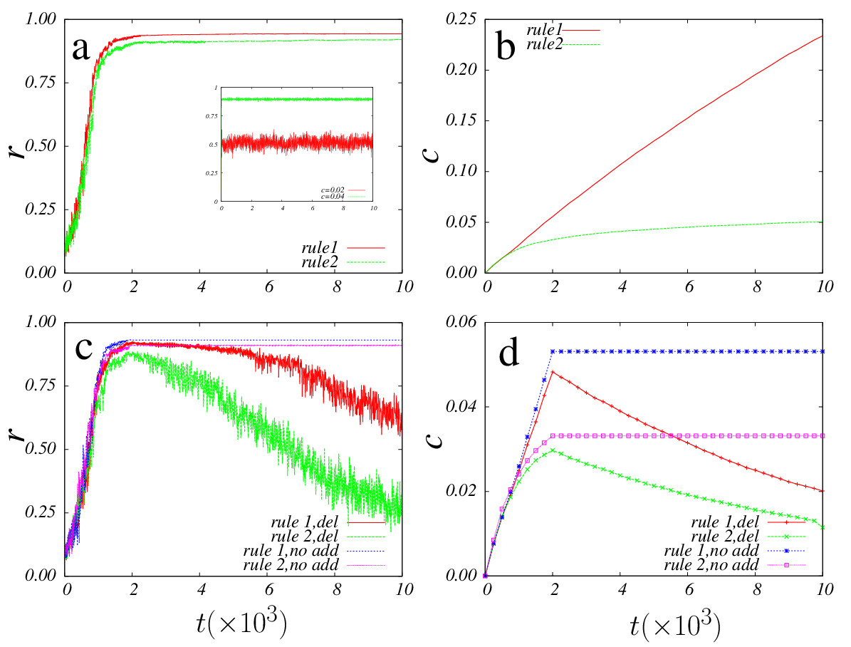
Fig. 1 shows the variation of order-parameter, and connection, with time, for global coupling strength, , for a system of size with the parameter of the waiting time distribution, . As observed from Fig. 1(a),(inset), it takes a comparatively longer time for the system of phase oscillators to reach a phase-locked state in an evolving network as compared to a network of static topology with a given connection density. Sublinear growth of with is shown in Fig. 1(b). We have evolved the system upto and observed that the connection density for both the transition rules. The exact value of exponent depends on the transition rules and the value of coupling strength. The time series for in the two figures also suggests towards existence of a threshold value of connection density in order to achieve global synchronization. To confirm the existence of a threshold value of connection density, we stop adding new links to the network once the system achieves global synchronization. We observe that the synchronization persists thereafter providing a strong indication towards the existence of a minimum number of oscillators which should interact so that the system evolves coherently as a whole. Once the network stops evolving, we check the robustness of the synchronized state and find that synchronization is not resilient to random removal of links as the network gets fragmented(see Fig. 1(c),(d)).

In Fig. 2 is the phase diagram vs show a monotonic increase of with . We observe that a threshold value of is required in order to achieve synchronization. Once the synchronization is achieved, becomes constant but rises due to addition of links on an average. Existence of a threshold value of can be understood from the observation that size of the largest connected component of the directed graph quickly becomes , the system size. This is achieved well before synchronization sets in. This also explains the desynchronization in the system due to random removal of links which makes the network fragmented into many components. This observation was confirmed by walking on the graph using depth first search algorithm, which provides the size of the connected components in a graph [15]. A threshold value of required for the system to achieve synchronization also suggests that a system of larger size will take longer time to achieve synchronization in comparison to a system of smaller size which is confirmed numerically. Numerically, exact value of threshold connection depends on the value of the order-parameter at which the system is considered to be synchronized, e.g., if is chosen to be the value of order-parameter for global synchronization, the corresponding threshold connection density is, .

Fig. 3 shows the evolution of degree distribution with time for the network. The mean of the degree distribution grows sublinearly in time with for both the transition rules. The equality of mean degree is evident from the fact that total in-degree equals total out-degree for a directed network and hence, every node is affected almost equally by its neighbors. Variances on the other hand are not identical for both the in- and out-degree distributions for rule 1, with the in-degree distribution showing less width in comparison to the out-degree distribution(Fig. 3(a),(b)). Note that for rule 1, , and since depends on the ratio of the out-degree of node to the sum of in-degree of node and out-degree of node . As a result different oscillators contribute differently towards affecting the dynamics of a given oscillator. However, for the second transition rule, we see that , therefore the width is identical for both the in- and out-degree distributions for obvious reasons.

Finite size scaling of the transition curve(Fig. 4) shows that the properties observed from numerical solution of Eq. (1) do not depend on system size. Finite size scaling analysis also provides an approximate value of the critical coupling strength, below which the system will never reach a phase locked state independent of its evolution time. The value of critical coupling strength is the same for both the transition rules and this can be understood in terms of the connection threshold. This is because once the system reaches synchronization, increasing connection density further does not have any significant effect on the order parameter. Furthermore, a finite value of critical coupling strength is also evident from the observation that the second moment of the degree distribution of the steady-state network is finite [16].
We benchmark our results against existing literature by solving the dynamical equations with oscillator frequencies distributed according to Cauchy distribution peaked at the origin and having scale parameter, . In the mean field limit for a completely connected graph, the critical value of coupling strength is, [3]. We evolve the network by adding links with probability one to randomly chosen pair of nodes so that the steady state topology of the network is that of a completely connected graph. We find , which provides a benchmark to our results.
In order to investigate the dependence of on the mean of the waiting time distribution , we looked at the variation of order-parameter with coupling for different values of for a fixed system size. We find that varying does not have any appreciable effect on the value of critical coupling strength for either of the rules. This observation suggests that is independent of .
To conclude, we have shown that the interdependence of topology and dynamics is necessary in order to understand how synchronization emerges collectively from local interactions in a self-organizing manner. This has real world implications for systems in which interactions keep changing with time but an overall rythm persists on an average. It is also observed in natural systems that the synchronous state does not persist forever. In this model we have provided a mechanism for collective emergence of synchronization from local dynamics. The synchronization achieved is characteristic of the network evolved by the transition rules. However, it is independent of the connection density of the network provided it is above a threshold. Existence of a connection density threshold in order to achieve synchronization has practical applications, e.g., from the context of Josephson junction arrays in reducing the number of redundant connection links in order to achieve desired output thereby minimizing the cost of wirings. We hope that this work provides an impetus for future work on synchronization from a dynamic perspective.
References
- [1] Y. Kuramoto., Lecture Notes in Physics 39, 420 (Springer, 1975); Y. Kuramoto and I. Nishikawa, J. Stat. Phys., 49, 569 (1987).
- [2] S. H. Strogatz, Physica D, 143, 1 (2000).
- [3] J. A. Acebron, L. L. Bonilla, C. J. P. Vicente, F. Ritort, and R. Spigler, Rev. Mod. Phys., 77, 137 (2005).
- [4] A. Pikovsky, M. Rosenbaum and J. Kurths, Synchronization: A Universal Concept in Nonlinear Science (Cambridge University Press, Cambridge, 2001).
- [5] S. H. Strogatz, Nature, 410, 268 (2001).
- [6] M. Barahona and L. M. Pecora, Phys. Rev. Lett. 71, 036151(2005); J. G. Restrepo, E. Ott, and B. R. Hunt, Phys. Rev. E, 71, 036151; D. Cummin and C. P. Unsworth, Physica D, 226, 181 (2007); A. Arenas, A. Díaz-Guilera, J. Kurths, Y. Moreno, and C. Zhou,Physics Reports 469 93 (2008); D. Witthaut and M. Timme, Phys. Rev. E., 90, 032917 (2014).
- [7] Y. Moreno and A. F. Pacheco, Europhys. Lett., 68, 603 (2004); Georgi S. Medvedev, Physica D, 266, 13 (2014).
- [8] P. Holme, J. Saramaki, Phys. Rep., 519, 97 (2012).
- [9] G. Su, Z. Ruan, S. Guan and Z. Liu, Europhys. Lett., 103, 48004 (2013); X. Zhang, S. Boccaletti, S. Guan and Z. Liu, Phys. Rev. Lett., 114, 038701 (2015).
- [10] R. Albert, H. Jeong and A. L. Barabasi, Nature, 406, 378 (2000); L. K. Gallos, P. Argyrakis, A. Bunde, R. Cohen, S. Havlin, Physica A, 344, 504 (2004); R. Cohen, K. Erez, D. Ben-Avraham, S. Havlin, Phys. Rev. Lett., 86, 3682 (2001).
- [11] R. Albert and A. L. Barabasi, Rev. Mod. Phys., 74, 47 (2002).
- [12] A. L. Barabasi, R. Albert, Science, 286, 509 (1999).
- [13] S. Redner, Eur. Phys. J. B, 4, 131 (1998).
- [14] M.E.J. Newman and G.T. Barkema, Monte Carlo Methods in Statistical Physics (Clarendon Press, Oxford, 1999).
- [15] S. Even, Graph Algorithms (Cambridge University Press, Cambridge, 2011).
- [16] T. Ichinomiya, Phys. Rev. E 70, 026116 (2004), Phys. Rev. E 72, 016109 (2005); D. S. Lee, Phys. Rev. E 72, 026208 (2005).