Transport in ultradilute solutions of 3He in superfluid 4He
Abstract
We calculate the effect of a heat current on transporting 3He dissolved in superfluid 4He at ultralow concentration, as will be utilized in a proposed experimental search for the electric dipole moment of the neutron (nEDM). In this experiment, a phonon wind will generated to drive (partly depolarized) 3He down a long pipe. In the regime of 3He concentrations and temperatures K, the phonons comprising the heat current are kept in a flowing local equilibrium by small angle phonon-phonon scattering, while they transfer momentum to the walls via the 4He first viscosity. On the other hand, the phonon wind drives the 3He out of local equilibrium via phonon-3He scattering. For temperatures below K, both the phonon and 3He mean free paths can reach the centimeter scale, and we calculate the effects on the transport coefficients. We derive the relevant transport coefficients, the phonon thermal conductivity and the 3He diffusion constants from the Boltzmann equation. We calculate the effect of scattering from the walls of the pipe and show that it may be characterized by the average distance from points inside the pipe to the walls. The temporal evolution of the spatial distribution of the 3He atoms is determined by the time dependent 3He diffusion equation, which describes the competition between advection by the phonon wind and 3He diffusion. As a consequence of the thermal diffusivity being small compared with the 3He diffusivity, the scale height of the final 3He distribution is much smaller than that of the temperature gradient. We present exact solutions of the time dependent temperature and 3He distributions in terms of a complete set of normal modes.
pacs
67.60.G- 13.40.Em 05.20.DdI Introduction
The physics underlying the transport properties of mixtures of 3He and superfluid 4He changes markedly as the concentration of 3He varies. We determine here the transport properties of these mixtures at very low concentrations, , where and are the 3He and 4He densities, and low temperatures, K, where phonons are the dominant superfluid excitation. In this case, the phonons are in local thermal equilibrium; their interactions with the 3He distort the 3He distribution and dominate the 3He diffusion. For concentrations , the reverse situation holds: the 3He are in local equilibrium due to rapid 3He–3He scattering and the phonon distribution is distorted due to phonon–3He interactions [1]. In the intermediate concentration regime, the phonon and 3He distributions are both distorted and must be determined by solving the coupled evolution, or Boltzmann, equations [2]. At the highest concentrations, %, Fermi-Dirac statistics for the 3He become important [3]. These transport properties are of interest as an example of a two-component fluid with excitations of comparable energy but very different momenta, and where the excitations of the two species obey different statistics.
The transport properties of 3He in superfluid 4He at low concentrations are also important for the proposed experiment [4] to measure the neutron electric dipole moment (nEDM) at the Oak Ridge National Laboratory Spallation Neutron Source. There, the neutron precession frequency will be determined using the absorption of polarized ultracold neutrons on polarized 3He atoms in solution in superfluid 4He via the reaction
| (1) |
which has a strong spin dependence, since capture proceeds primarily through the spin-singlet channel. Two key considerations accrue from this choice of detection technique. In order to maximize the precision with which the precession frequency can be measured, the optimal 3He concentration, , corresponds to a capture rate comparable to the decay rate of the neutrons. However, primarily due to wall collisions, the 3He will gradually become depolarized. In order to reduce the background from neutron capture on unpolarized 3He, it is crucial to be able to periodically sweep out the 3He by means of a heat current [5]. In this paper, we calculate both the heat and 3He particle currents based on well-established microscopic theory of phonon–phonon [6] and phonon–3He scatterings [7], as well as the evolution of both the temperature and 3He concentration.
At the concentrations and temperatures of interest in the experiment, in addition to phonon-phonon, phonon-3He and 3He–3He scattering, the scattering of both phonons and 3He from the walls of the containers can also be important. Here we extend the solution of the Boltzmann equations in Ref. [2] to include these effects, in addition to providing some examples for . For illustration, we consider the effect of a heat current in an essentially one dimensional geometry, with the 3He superfluid 4He mixture in a long pipe with a diameter of a few cm. The phonon-wall interactions affect the thermal conductivity as well as the phonon velocity distribution within the pipe; the 3He–wall interactions affect the transport of the 3He in the presence of a heat current.
This paper is arranged as follows: Section II describes the basic scattering mechanisms the calculation of transport coefficients from the Boltzmann equation is given in Sec. III. Subsequently, we calculate the temporal and spatial evolution of the temperature (Sec. IV) and the 3He density (Sec. V). We summarize results in Sec. VI. In Appendix A we analyze the transport when scattering of phonons is predominantly from the walls of the pipe, and in Appendix B we solve analytically the equation for the temporal evolution of the 3He concentration.
II Phonon and 3He relaxation
We begin by considering the relevant microscopic relaxation mechanisms (detailed in Ref. [2]), first for the phonons. The momentum-dependent mean free path of a phonon of momentum scattering against the 3He,
| (2) |
is typically greater than 1 km for and K [2]; here is the corresponding scattering rate, is the phonon velocity, and is an angle-integrated rate constant. Therefore, phonon–wall and phonon–phonon scatterings determine the phonon distribution. As discussed in Refs. [2] and [9], rapid, small angle phonon-phonon scattering establishes thermal equilibrium along phonon ‘rays,’ i.e., given directions in momentum space, with the distribution
| (3) |
where is the local temperature and is the mean phonon drift velocity. Large angle phonon-phonon scattering, either in a single event or a succession of small-angle processes, is slower and gives rise to the phonon first viscosity,
| (4) |
where is the phonon entropy density and is the viscous mean free path. At a pressure of bar,
| (5) |
to a good approximation [6, 10], where is the temperature in Kelvin; at = 0.45 K, 0.17 cm.
In the presence of a heat flux, , small-angle phonon-phonon scattering keeps the phonons in local thermal equilibrium, where the mean phonon drift velocity, , is
| (6) |
The thermal conductivity of the phonons, , can, at low concentrations, be written as [2, 10],
| (7) |
in a pipe of radius and where is the effective mean free path
| (8) |
The second term represents scattering of the phonons on the walls; the numerical coefficient 16/5 is chosen to give the correct Casimir limit. In this limit, large compared to the pipe diameter (see Appendix A), the phonon thermal conductivity assumes the Casimir form [11]
| (9) |
In the opposite limit, , the thermal conductivity becomes
| (10) |
The 3He contribution to the overall heat flux is negligible at low [1, 2].
The mean free path of a 3He scattering on unpolarized 3He is [2]
| (11) |
where is the corresponding cross section. Thus for , one has m; we therefore neglect 3He–3He scattering. On the other hand, the mean free path for 3He scattering on phonons [2],
| (12) | |||||
where is the 3He effective mass in superfluid 4He, is small compared to the pipe diameter for K. Thus the dominant process for bringing the 3He toward equilibrium for temperatures of interest in the experiment is scattering against phonons. In the next section, we outline the calculation of the 3He transport coefficients; more details can be found in Ref. [2].
III Boltzmann equation and transport coefficients
The 3He Boltzmann equation has the general form
| (13) |
Here is the 3He distribution function,
| (14) |
is the equilibrium distribution function, and we write the deviations from local equilibrium as
| (15) |
where
| (16) |
is the local equilibrium distribution function, i.e., the distribution towards which collisions with phonons drive the 3He. The first term on the right represents the scattering on the phonons, the second term the scattering from other 3He (numerically insignificant for the concentrations of interest) and the last two terms isotropic diffuse (d) and specular (s) scattering of the 3He from the walls. In the term describing collisions with phonons, and are the initial and final 3He momenta, respectively, and and are the corresponding phonon momenta. The phonon–3He scattering kernel is , and momentum conservation, , is understood in the collision term.
In order to calculate the effects of a phonon wind on the 3He we solve Eq. (13) for . On the left side of the Boltzmann equation, we approximate the distribution by its local equilibrium form, . We neglect the contribution from because of the relatively small temperature gradient (see Eq. (38) below), while the gradient of in this term gives a second order contribution, which we neglect. The left side of the Boltzmann equation is then
| (17) |
On the right side we write
| (18) |
as shown in Ref. [2] the 3He-phonon collision term is diagonalized by expanding in Sonine polynomials [2].
To solve for we multiply the Boltzmann equation by and integrate over all . Noting that the distortion is proportional to , we see first that on the right side of the Boltzmann equation the two term do not contribute, since both the 3He–3He scattering and the specular 3He scattering from the walls conserve momentum in the z direction. Following Eq. (81) of Ref. [2] for the phonon-3He scattering, we see that the remaining terms on the right side comprise
| (19) |
With the inclusion of the recoil effect in the phonon–3He scattering to lowest order (see the Appendix of Ref. [1] and Sec. 6 of Ref. [2]), the solution of the Boltzmann equation is
| (20) |
where
| (21) |
is the effective 3He scattering rate, including both scattering from phonons, encoded in , and diffuse scattering from the walls of the pipe.
Integrating the Boltzmann equation, Eq. (13), over we recover the continuity equation
| (22) |
with the 3He particle current given by
| (23) |
where is the number of spin degrees of freedom of the 3He: 1 for a fully polarized sample and 2 in the unpolarized case. It is straightforward to evaluate the current (including the effect of recoil in the phonon–3He scattering)
| (24) |
where the 3He diffusion constant, including recoil corrections, is [2]
| (25) |
and the “thermoelectric” coefficient is
| (26) |
In these expressions the basic forms of and are modified by the wall scattering factor
| (27) |
where
| (28) |
is the fraction of the 3He wall scattering rate that is diffuse.
To see the effect of scattering of 3He from the walls, we take the total wall scattering rate to be simply
| (29) |
where is the mean 3He thermal velocity, and [see Eq. (62)] is the effective average distance from an interior point to the wall of an infinitely long pipe of radius entering the transport [13]. The effect of wall scattering on the diffusion constant, , for example, is shown in Fig. 1 for . As we see, the effect becomes more important for lower temperatures because of the decrease in the phonon density. As , approaches the result without wall scattering, which in the vicinity of the operating temperature regime of the nEDM experiment, K, is
| (30) |
We also show, in Fig. 2, the corresponding effect of phonon–wall scattering on the phonon thermal conductivity, Eq. (7).


At temperatures of approximately 0.3K and below, the mean free path of a 3He quasiparticle in the bulk medium is greater than 1 cm, which is comparable to the radii of the pipes considered for the nEDM experiment. In this regime, the 3He quasiparticles can lose momentum not only by collisions with phonons but also directly to the walls of the pipe. This situation is analogous to the (Knudsen) flow of a low-density gas in response to a pressure gradient, except that in the dilute helium solutions the force driving the flow of 3He has two components, one due to the 3He pressure gradient and another due to the collisions with phonons. When the 3He distribution function is stationary, the two contributions to the force are equal and opposite. The 3He distribution function in principle depends not only on direction in momentum space but also on the radial coordinate in the pipe. However, the time scales for smoothing out the radial dependence via diffusion or ballistic transport are of order several milliseconds, and therefore short compared with the overall evolution time scales of the system. A detailed study of this regime lies outside the scope of the present article.
IV Time evolution of the temperature
We now estimate, using the heat diffusion equation. the timescale for heating the fluid. We assume, as above, that the heat is carried by the phonons (see also Eq. (89) of Ref. [2] and discussion following) and that the relative temperature variation and, hence, the variation of is small, so that
| (31) |
where is phonon energy density. Within a few scattering times after the application of heat at one end of the pipe (), the temperature there is approximately fixed at . We assume that the temperature at , the other end of the pipe, is kept constant at temperature by a refrigerator.
To solve the heat diffusion equation it is sufficient to consider the average of the temperature, , over the cross-section of the pipe, thus avoiding having to take into account details of the counterflows within the pipe. The solution is given in terms of the modes in the pipe that vanish at and , , where , with here a positive integer:
We denote the thermal diffusivity by
| (33) |
and recognize as the 4He specific heat. The condition that except immediately at , implies that the mode weights are given by . The characteristic time, , to set up a steady state phonon wind is essentially that of the mode,
| (34) |
For typical conditions in the experiment, 5 mW of heat in a 3 cm diameter, 100 cm long pipe at K, the phonon thermal conductivity is erg/scmK, ms, and mK.
V Time evolution of the concentration
To begin examining the 3He concentration, we consider its steady-state distribution in the presence of a heat current or phonon wind. Because, as we shall see below, the term involving is relatively small for low concentrations, the condition that the 3He particle current, Eq. (24), vanishes, is simply
| (35) |
which has the solution
| (36) |
where we define the scale height, (for the example parameters above, cm2/s, cm/s and cm), and
| (37) |
with the initial uniform 3He density. We note that the relative size of the term involving is simply the ratio of the scale heights of the concentration and the temperature,
| (38) |
about 1/1000 for the example parameters given above.
In the nEDM experiment, the 3He in the system depolarizes in time, primarily due to interactions with walls. The depolarized 3He will be removed by a phonon wind before the system is recharged with more highly polarized 3He. As above, we consider the simple situation of a long pipe with a heater at and closed ends. The evolution of the 3He is governed by a competition between two processes: the phonon wind, which were it to act alone would push all the 3He to the downstream (large ) end of the pipe, and diffusion of the 3He, limited by scattering with the phonons, which allows the 3He to drift back towards smaller .
This evolution of the 3He concentration in the presence of a phonon wind is described by the diffusion equation resulting from Eq. (22),
| (39) |
where we have dropped the term in Eq. (24). Once a steady phonon wind, with a small temperature gradient, is established, we may neglect the temperature dependence of and take and to be constant. For a pipe with a large length to diameter ratio, we may treat the problem as one dimensional, averaging over its cross section as we did above for the heat flow. The boundary conditions are that the 3He current, , Eq. (24), vanishes at the two ends of the pipe,
| (40) |
To solve Eq. (39) with constant and , we write the 3He density as and decompose as a sum of time dependent modes periodic in (see Appendix B):
| (41) |
where satisfies the boundary condition
| (42) |
The spatial parts of the mode functions are the complete orthonormal set
| (43) |
with and . The time dependence of the modes is where
The solution of Eq. (39) for an initially uniform density is then
| (48) |
where
As we show in Appendix B, the general solution may be written in compact form in terms of a Green’s function
| (53) |
where
| (54) |


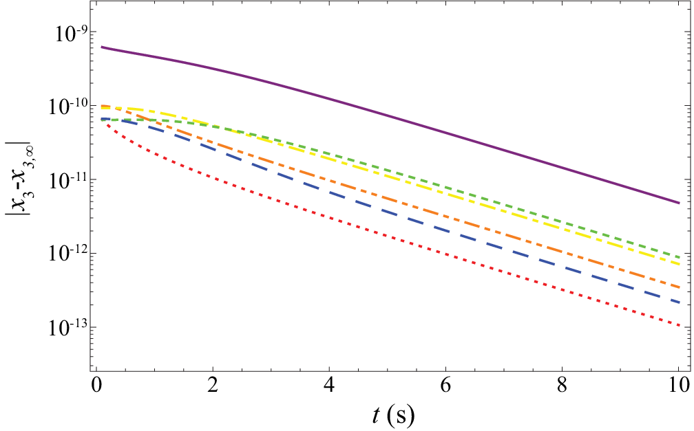
The and dependences of are shown in Figs. 3 and 4, respectively, for the case of the uniform initial distribution and typical experimental values (5 mW heat into a 3 cm diameter, 100 cm long pipe at K). As the figures illustrate, the concentration scale height, , is substantially smaller than the pipe length. Figure 5 plots the difference between and its steady state value for several points along the pipe, showing that, after a few seconds, the lowest mode, with s, dominates the time evolution throughout the pipe.
The results for the evolution of the 3He concentration presented here are equally applicable to a heat flush experiment being carried out at Harvard at natural 3He concentration [14]. There one must use the more general phonon thermal conductivity as derived in [2]; phonon-wall scattering in this regime plays a negligible role.
VI Summary
We have calculated the transport properties of dilute mixtures, , of 3He in superfluid 4He at temperatures around 0.5 K where phonons are the dominant excitations of the superfluid. In this regime, we considered a simple one dimensional geometry (a pipe), a heat current generates a phonon wind with phonons in local equilibrium corresponding to the temperature at that point in the pipe. On the other hand, phonon scattering distorts the 3He distribution from equilibrium. Starting from the known phonon–phonon and phonon–3He scattering, we calculate the transport coefficients from the Boltzmann equation. We show that, in the presence of a heat current which generates a temperature scale height much larger than the length of the pipe (i.e., a small relative temperature gradient), the scale height for the 3He concentration can be much less than the pipe length. This leads to a large decrease in concentration at the hot boundary and a corresponding increase at the cold end. For temperatures below K the mean free paths of both the phonons and the 3He can reach the centimeter scale; in these cases, scattering from the walls of the container becomes important. Finally, we calculate the timescales associated with the evolution of both the temperature and concentration distributions; because of the large superfluid thermal conductivity, the thermal timescales are on the ms scale, whereas the corresponding scale for evolution of the concentration is on the scale of seconds.
Acknowledgements
This research was supported in part by NSF Grants PHY-1205671 and PHY-1305891. GB is grateful to the Aspen Center for Physics, supported in part by NSF Grant PHY-1066292, and the Niels Bohr International Academy where parts of this research were carried out, and he thanks Hiroshi Fukuyama for enlightening discussions. DB thanks Caltech, under the Moore Scholars program, and CJP thanks Andrew Jackson for helpful comments.
Appendix A Phonon drift velocity in the ballistic limit
Here we derive the spatial dependence of the phonon drift velocity when the phonon-phonon scattering mean free path for large angle scattering, Eq. (5), is much larger than the pipe radius, . For the pipe geometry considered in the text, this condition holds at a temperature K. We assume that the pipe axis is in the z direction, and that the transverse coordinates are and . We also assume that a phonon striking the cylinder wall is diffusively reflected, with a distribution of final momenta given by the local temperature, , where is the temperature gradient. Then , the number of phonons of momentum at point , is given by the equilibrium distribution at the point on the pipe wall where the phonon at originated:
| (55) |
to lowest order in , where is the equilibrium distribution.
The point of origin is determined by simple geometry, namely, , where . We measure in polar coordinates and . Then , , and . Using on the cylinder wall, we have then
where is the azimuthal angle of and . The solution is
| (57) |
without loss of generality we take .
The local phonon flow velocity is given by the local total momentum flux density in the z direction divided by the normal mass density of the phonons, ,
| (58) |
To first order in , only the term in the distribution function survives the angular average in the numerator, so that
| (59) |
independent of . Since is independent of , the integrals over in numerator and denominator cancel, and
| (60) |
where the angular brackets denote the average over angles of .
The flow velocity averaged over the cross section of the pipe (denoted by an overline) is simply
where
| (62) |
In evaluating , the integral over decouples from those over and , and the latter are easily performed if one integrates over before integrating over . One finds
| (63) |
which expresses the fact that the length important for thermal conduction is one half of , the average distance to the wall of the pipe, averaged over the cross section of the pipe. Since , where is the phonon heat capacity, we find the phonon thermal conductivity,
| (64) |
which is the Casimir result, Ref. [11].
Locally,
| (65) |
where the elliptic integral,
| (66) |
must be done numerically. As we see in Fig. 6 the velocity profile
| (67) |
is independent of and nearly quadratic almost to the edge of the pipe, where it falls more rapidly, but unlike when viscosity dominates, it does not fall to zero at the pipe wall.

Appendix B Exact solution of the time dependent diffusion equation with advection
Here we construct the general solutions of the time-dependent diffusion equation (39) by first transforming the equation into self-adjoint form by writing . As a result, obeys
| (68) |
in the interval (we simply write a generic diffusion constant, , to simplify the notation). The boundary condition of vanishing current at the two ends of the pipe then becomes
| (69) |
where . To realize the boundary conditions we expand in a complete set of normalized solutions of Eq. (68) that are periodic in the interval 0 to ,
| (70) |
with (), and
| (71) |
together with the stationary solution
| (72) |
The modes form an orthonormal set obeying
| (73) |
as well as the completeness relation in the interval ,
| (74) |
The time dependence of the modes is , with
| (75) |
and . Then
| (76) |
with
| (77) |
We can thus write the solution in terms of the initial density distribution as
| (78) |
where
| (79) |
is the Green’s function for the diffusion equation in the form (68), with the Helmholtz unit step function. At , the completeness relation implies , and thus
| (80) |
in the interval .
References
- [1] G. Baym, D. H. Beck, and C. J. Pethick, Phys. Rev. B 88, 014512 (2013), arXiv:1212.2946.
- [2] G. Baym, D. H. Beck, and C. J. Pethick, J. Low Temp. Phys., 178, 200 (2015); arXiv:1408.1619.
- [3] G. Baym, J. Bardeen and D. Pines, Phys. Rev. 156, 207 (1967); G. Baym and C. J. Pethick, Landau Fermi liquid theory: concepts and applications, (J. Wiley and Sons, New York, 1991).
- [4] R. Golub and S. K. Lamoreaux, Phys. Rep. 237, 1 (1994).
- [5] M. Hayden, S. K. Lamoreaux, and R. Golub, AIP Conf. Proc. 850, 147 (2006).
- [6] H. J. Maris, Rev. Mod. Phys. 49, 341 (1977).
- [7] G. Baym and C. Ebner, Phys. Rev. 164, 235 (1967).
- [8] The measurement is optimized when the neutron capture rate is approximately the same as the neutron decay rate—this occurs for concentrations .
- [9] D. Benin and H. J. Maris, Phys. Rev. B 18, 3112 (1978).
- [10] D. Greywall, Phys. Rev. B 23, 2152 (1981).
- [11] H. B. G. Casimir, Physica 5, 495 (1938). A basic assumption here is that phonons leaving the walls of the tube are in thermal equilibrium at the local temperature of the wall. If there is significant specular reflection at the wall, the result is modified.
- [12] S. K. Lamoreaux, G. Archibald, P. D. Barnes, W. T. Buttler, D. J. Clark, M. D. Cooper, M. Espy, G. L. Greene, R. Golub, M. E. Hayden, C. Lei, L. J. Marek, J.-C. Peng, and S. Penttila, Europhys. Lett. 58, 718 (2002).
- [13] For wall scattering alone, the diffusion constant would be simply , where is the average mean free path, here simply , the pipe diameter..
- [14] D. H. Beck et al. (to be published).