Comparing persistence diagrams through complex vectors

Persistent homology has already proven to be an effective tool for shape representation in various applications, in particular when the objects to be classified, compared or retrieved have a natural origin. The interplay of geometry and topology in persistence makes it possible to capture qualitative aspects in a formal and computable way, yet it doesn’t suffer of the excessive freedom of mere topological equivalence. The privileged tool for shape comparison is the natural pseudo-distance [11], which is scarcely computable. Luckily, persistence diagrams condense the essence of the shape concept of the observer in finite sets of points in the plane [16, 13]; moreover, the bottleneck distance (a.k.a. matching distance) between persistence diagrams yields an optimal lower bound to the natural pseudo-distance [9, 10]. There is a problem: the bottleneck distance suffers from combinatorial explosion [8], so it becomes hard to scan a large database when it comes to retrieval. Approximations, smart organization of the database according to the metric, progressive application of different classifiers come to help, but the problem is lightened, not solved.

A paradigm shift came from an idea of Claudia Landi [15]: represent the persistence diagram as the set of complex roots of a polynomial; then comparison can be performed on coefficients. Two problems arise: one — which comes from the nature itself of persistence diagrams — is that in real situations there are a lot of points near the “diagonal” $\{(u,v)\in\mathbb{R}^{2}:u=v\}$, due to noise so less meaningful in shape representation, but with a heavy impact on polynomial coefficients; another problem — coming from polynomial theory — is that little distance of polynomial roots implies little distance of coefficients, but the converse is false.

A completely different polynomial representation of barcodes (equivalently: of persistence diagrams) is the one through tropical algebra [17], closely adapting to the bottleneck distance.

In persistence, the shape of an object is usually studied by choosing a topological space $X$ to represent it, and a function $f:X\to\mathbb{R}$, called a filtering (or measuring) function, to define a family of subspaces $X_{u}=f^{-1}((-\infty,u])$, $u\in\mathbb{R}$, nested by inclusion, i.e. a filtration of $X$. The name “persistence” is bound to the idea of ranking topological features by importance, according to the length of their “life” through the filtration. The basic assumption is that the longer a feature survives, the more meaningful or coarse the feature is for shape description. In particular, structural properties of the space $X$ are identified by features that once born never die; vice-versa, noise and shape details are characterized by a short life. To study how topological features vary in passing from a set of the filtration into a larger one we use homology. A nice feature of this approach is modularity: The choice of different filtering functions may account for different viewpoints on the same problem (different shape concepts) or for different tasks. For further details we refer to [1, 12].

Persistent homology groups of the pair $(X,f)$ — i.e. of the filtration $\{X_{u}\}_{u\in\mathbb{R}}$ — are defined as follows. Given $u\leq v\in\mathbb{R}$, we consider the inclusion of $X_{u}$ into $X_{v}$. This inclusion induces a homomorphism of homology groups $H_{k}(X_{u})\rightarrow H_{k}(X_{v})$ for every $k\in\mathbb{Z}$. Its image consists of the $k$-homology classes that are born before or at the level $u$ and are still alive at the level $v$ and is called the $k$th persistent homology group of $(X,f)$ at $(u,v)$. When this group is finitely generated, we denote by $\beta_{k}^{u,v}(X,f)$ its rank.

The usual, compact description of persistent homology groups of $(X,f)$ is provided by the so-called persistence diagrams, i.e. multisets of points whose abscissa and ordinate are, respectively, the level at which $k$-homology classes are created and the level at which they are annihilated through the filtration. If a homology class does not die along the filtration, the ordinate of the corresponding point is set to $+\infty$.

At the moment, our approach to convert persistence diagrams into complex vectors can be applied only when neglecting these points at infinity. Hence, we focus on the subsets of proper points of the classical persistence diagrams, known in literature as ordinary persistence diagrams [6]. For simplicity we still call them “persistence diagrams”. We underline that this choice is not so restrictive since the number of points at infinity depend only on the homology of the space $X$, and persistent homology provide a finite distance between two pairs if and only if the considered spaces are homeomorphic.

We use the following notation: $\Delta^{+}=\{(u,v)\in\mathbb{R}^{2}:u<v\}$, $\Delta=\{(u,v)\in\mathbb{R}^{2}:u=v\}$, and $\overline{\Delta^{+}}=\Delta^{+}\cup\Delta$.

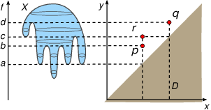
Figure 1 displays an example of persistence diagram for $k=0$. The surface $X\subset\mathbb{R}^{3}$ is filtered by the height function $f$. $D_{0}(X,f)$ has three proper points $p_{1},p_{2},p_{3}$ since the abscissa of these points corresponds to the level at which new connected components are born along the filtration, while the ordinate identifies the level at which these connected components merge with existing ones. In terms of multiplicity, this means that $\mu_{0}(p_{i})>0$, $i=1,2,3$, and $\mu_{0}(p)=0$ for every other point $p\in\Delta^{+}$. To see, for example, that $\mu_{0}(p_{1})=2$, where $p_{1}=(a,b)$, it is sufficient to observe that, for every $\varepsilon>0$ sufficiently small, it holds that $\beta_{0}^{a+\varepsilon,b-\varepsilon}(X,f)=4$, $\beta_{0}^{a+\varepsilon,b+\varepsilon}(X,f)=2$, $\beta_{0}^{a-\varepsilon,b-\varepsilon}(X,f)=\beta_{0}^{a-\varepsilon,b+\varepsilon}(X,f)=1$, and apply Definition 1. In an analogous way, it can be observed that $\mu_{0}(p_{2})=\mu_{0}(p_{3})=1$.

Persistence diagrams comparison is usually carried out through the so called bottleneck distance because of the robustness of these descriptors with respect to it. Roughly, small changing in a given filtering function (w.r.t. the max-norm) produces just a small changing in the associated persistence diagram w.r.t. the bottleneck distance [7, 4]. The bottleneck distance between two persistence diagrams measures the cost of finding a correspondence between their points. In doing this, the cost of taking a point $p$ to a point $p^{\prime}$ is measured as the minimum between the cost of moving one point onto the other and the cost of moving both points onto the diagonal. In particular, the matching of a proper point $p$ with a point of $\Delta$ can be interpreted as the destruction of the point $p$. Formally:

Driven by the awareness that, in the experimental framework, evaluating the bottleneck distance can be computationally expensive, making its usage not practicable on large datasets, in this work we propose a new procedure based on the preliminary idea introduced in [15]. We translate the problem of comparing directly two persistence diagrams through the bottleneck distance into the problem of comparing complex vectors associated with each persistence diagram through appropriate metrics between vectors. The components of these complex vectors are complex polynomials’ coefficients obtained as follows. Firstly, we define a certain transformation taking points of persistence diagrams to the set of complex numbers. Secondly, we construct a complex polynomial having the obtained complex numbers as roots.

In this paper, we consider the three transformations below:

• –

  $R:\overline{\Delta^{+}}\to\mathbb{C}$, with $R(u,v)=u+iv$,

• –

  $S:\overline{\Delta^{+}}\to\mathbb{C}$, with $S(u,v)=\left\{\begin{array}[]{ll}\dfrac{v-u}{\alpha\sqrt{2}}\cdot(u+iv),&\mbox{if}\,(u,v)\neq(0,0)\\ (0,0),&\mbox{otherwise}\end{array}\right.$,

• –

  $T:\overline{\Delta^{+}}\to\mathbb{C}$, with $T(u,v)=\dfrac{v-u}{2}\cdot(\cos\alpha-\sin\alpha+i(\cos\alpha+\sin\alpha))$,

where $\alpha=\sqrt{u^{2}+v^{2}}$.

$R,S,T$ are continuous maps; $R$ and $S$ are also injective on $\overline{\Delta^{+}}$ and $\Delta^{+}$, respectively. We define the multiplicity of a complex number in the range of $R,S,T$ to be the sum of the multiplicities of the points belonging to its preimage (this is necessary because of the non-injectivity of $T$ on $\Delta^{+}$, although a preimage containing more than one proper point of the diagram has zero probability to occur). The main differences among these deformations are the following: the deformation $R$ acts as the identity, just passing from $\mathbb{R}^{2}$ to $\mathbb{C}$; the deformation $S$ warps the diagonal $\Delta$ to the origin, and takes points of $\Delta^{+}$ to points of $\{z\in\mathbb{C}:Re(z)<Im(z)\}$; the deformation $T$ warps the diagonal $\Delta$ to the origin, and takes points of $\Delta^{+}$ to points of $\mathbb{C}$. An example showing how $S$ and $T$ transform a persistence diagram is represented in Figure 2.

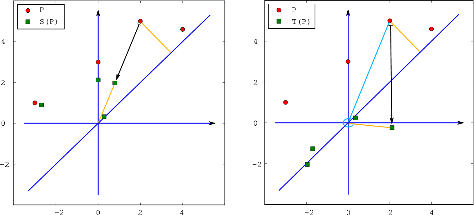
Both $S$ and $T$ seemed to be preferable to $R$ because points near $\Delta$ — due to noise — have to be considered close to each other in the bottleneck distance, although they may be very far apart in Euclidean distance. Taking them to be all near the origin would then also reduce their impact in the sums and sums of products which will build the polynomial coefficients we are going to compare. In particular, $T$ was designed to distribute the image of those noise points around zero, whereas $S$ makes them near zero, but all on one side: in the half-plane of $\mathbb{C}$ corresponding to $\Delta^{+}$. $T$ has two drawbacks: it is not injective on $\Delta^{+}$ and does not behave well with respect to simple transformations.

Let $D$ be a persistence diagram, and $p_{1}=(u_{1},v_{1}),\ldots,p_{s}=(u_{s},v_{s})$ its proper points with multiplicity $r_{1},\ldots,r_{s}$, respectively. Let now the complex numbers $z_{1},\ldots,z_{s}$ be obtained from $p_{1},\ldots,p_{s}$ by one of the transformations $R$, $S$ or $T$. We associate to $D$ the complex polynomial $f_{D}(t)=\prod_{j=1}^{s}(t-z_{j})^{r_{j}}$. We are actually interested in the coefficient sequence of $f_{D}(t)$, which we can compute by Viète’s formulas (see Algorithm 2).

Once we have the polynomials $f_{D}(t)=t^{n}-a_{1}t^{n-1}+\cdots+(-1)^{i}a_{i}t^{n-i}+\cdots+(-1)^{n}a_{n}$ and $f_{D^{\prime}}(t)=t^{m}-a^{\prime}_{1}t^{m-1}+\cdots+(-1)^{j}a^{\prime}_{j}t^{m-j}+\cdots+(-1)^{m}a^{\prime}_{m}$ corresponding to persistence diagrams $D$, $D^{\prime}$, we face a first problem, given by the possibly different degrees $n$ and $m$ ($m<n$ say). Because of their expression in terms of roots, we prefer to compare coefficients with the same index, rather than coefficients relative to the same degree of $t$. We manage this problem by adding $n-m$ null coefficients to $f_{D^{\prime}}(t)$, i.e. multiplying $f_{D^{\prime}}(t)$ by $t^{n-m}$, which amounts to adding the complex number zero with multiplicity $n-m$. In so doing, we can build two vectors of complex numbers $(a_{1},\dots,a_{n}),(a^{\prime}_{1},\ldots,a^{\prime}_{n})$ of the same length and are ready to compute a distance between them. By continuity of Viète’s formulas, close roots imply close coefficients. Hence, two persistence diagrams that are close in terms of bottleneck distance have close associated polynomials. Unfortunately, the converse is not true.

Preliminary tests suggested that the first coefficients were more meaningful; therefore we experimented with different distances on two complex vectors $(a_{1},\dots,a_{k}),(a^{\prime}_{1},\ldots,a^{\prime}_{k})$, $k\in\{1,\ldots,n\}$, one treating all coefficients equally, two which give decreasing value to coefficients of increasing indices. The chosen metrics are the following:

Let $N=|L|=|Db|$. It is easily seen that the computational complexities of Algorithms 1 and 3 are $C_{1}=O(M\cdot N)$ and $C_{3}=O(k\cdot N^{2})$, respectively. The cost of Algorithm 2 depends on how we have implemented the computation of Viète formulas. Using the induction on the index $j$, we have $C_{2}=O((2k^{2}+k\cdot M)\cdot N)$.

We want to show that our approach to database classification, in general, results to be cheaper than using the bottleneck distance by a suitable choice of the number $k$ of computed coefficients. Our comparison is realized in terms of storage locations and not in terms of running time performances since the algorithm proposed here and the one based on the bottleneck distance run on different platforms. We recall that the cost of computing the bottleneck distance $d_{B}(D,D^{\prime})$ is $C_{B}=O\left((r+r^{\prime})^{3/2}\log(r+r^{\prime})\right)$ if $A,A^{\prime}$ are the subsets of proper points of two persistence diagrams $D,D^{\prime}$ with $|A|=r,|A^{\prime}|=r^{\prime}$ (see [14]). Instead, using our scheme, with $N=2$ and $M=\max(r,r^{\prime})$, we get $O((\max(r,r^{\prime})+2k^{2}+k\cdot\max(r,r^{\prime})+2k)$, so $C=O(k\cdot(\max(r,r^{\prime})+k))$. Since $k\leq\max(r,r^{\prime})$, in the worst case, we have $C=O\left((\max(r,r^{\prime}))^{2}\right)$ which is higher than $C_{B}$, but for pre-processing we may choose a favorable $k$ (e.g. $k=\left\lfloor\sqrt{\max(r,r^{\prime})}\right\rfloor$). Also consider that, for a retrieval task, the heavy part of the computation (Viète’s formulas) for the database is performed offline; in other words: if we store the coefficient vectors instead of the proper points lists, then the search can be performed by a distance computation of complexity $O\left(\max(r,r^{\prime})\right)$!

This section is devoted to validate the theoretical framework introduced in Section 3. In particular, through some experiments on persistence diagrams for 0th homology degree associated with 3D-models represented by triangle meshes, we will prove that our approach allows to perform the persistence diagrams comparison without greatly affecting (and in some cases improving) the goodness of results in terms of database classification.

To test the proposed framework we considered a database of 228 3D-surface mesh models introduced in [2]. The database is divided into 12 classes, each containing 19 elements obtained as follows: A null model taken from the Non Rigid World Benchmark [3] is considered together with six non-rigid transformations applied to it at three different strength levels. An example of the transformations and their greatest strength levels is given in Figure 4.

Two filtering functions $f_{L}$, $f_{P}$ have been defined on the models of the database as follows: For each triangle mesh $M$ of vertices $\{v_{1},\dots,v_{n}\}$, the center of mass $B$ is computed, and the model is normalized to be contained in a unit sphere. Further, a vector $w$ is defined as

The function $f_{L}$ is the distance from the line $L$ parallel to $w$ and passing through $B$, while the function $f_{P}$ is the distance from the plane $P$ orthogonal to $w$ and passing through $B$ (see, as an example, Figure 4). The values of $f_{L}$ and $f_{P}$ are then normalized so that they range in the interval $[0,1]$. These filtering functions are translation and rotation invariant, as well as scale invariant because of a priori normalization of the models. Moreover, the considered models are sufficiently generic (no point-symmetries occur etc…) to ensure that the vector $w$ is well-defined over the whole database, as well as its orientation stability.

Our experimental results are synthesized in Tables 1 and 2 in terms of precision/recall (PR) graphs when the filtering functions $f_{L},f_{P}$, respectively, are considered. Before going into details, we want to emphasize that our intent is not to validate the usage of persistence for shape comparison, retrieval or classification. In fact, as a reader coming from the retrieval domain will probably note, the PR graphs reported in this paper are below the state of the art. This depends on the fact that, in general, good retrieval performances can be achieved only taking into account different filtering functions that give rise to a battery of descriptors associated with each model in the database.

What these plots aim to show is the comparison of the performances when the database classification is carried out through the computation of the bottleneck distance $d_{B}$ between persistence diagrams or the computation of the distances $d_{1}$, $d_{2}$ and $d_{3}$ between the first $k$ components of the complex vectors obtained through the transformations $R$, $S$ and $T$, for different values of $k$ (see Section 3 for the definitions of $R$, $S$, $T$, $d_{1}$, $d_{2}$ and $d_{3}$). As it can be easily observed, increasing the value of $k$ from the smallest to the biggest number of proper points in the persistence diagrams of our database, the PR graphs do not change so sensibly. This means that the most important information of the persistence diagram is contained in the first few vector components, the ones corresponding to the coefficients of monomials with highest degree. Moreover, we point out also that PR graphs related to vectors which are induced by transformations warping the diagonal $\Delta$ to a point (second and third rows in Tables 1 and 2) provide better results than by acting as the identity (first row). This fact depends on the properties of polynomial coefficients: Indeed roots corresponding to points of persistence diagrams farther from the diagonal weigh more than those closer to it. Hence, applying transformations $S$ and $T$ corresponds, in some sense, to providing points of a persistence diagram with a weight that follows the paradigm of persistence: The longer the lifespan of a homological class, the higher the weight associated with the point having as coordinates the birth and death dates of this class. This outcome is moreover strengthened by the usage of the distance $d_{3}$ (third column in Tables 1 and 2) since it greatly enhances the contribution of the first vector components to their dissimilarity measure at the expense of the last.

Finally, note that the precision values at high recall — i.e. by retrieving a large number of objects — are always fairly comparable with the values relative to the bottleneck distance. This assures us that complex vector comparison can act as a fast and reliable preprocessing scheme for reducing the set of objects to be fed to the generally more precise bottleneck distance.

References

- [1] Biasotti, S., De Floriani, L., Falcidieno, B., Frosini, P., Giorgi, D., Landi, C., Papaleo, L., Spagnuolo, M.: Describing shapes by geometrical-topological properties of real functions. ACM Comput. Surv. 40(4), 1–87 (2008)
- [2] Biasotti, S., Cerri, A., Frosini, P., Giorgi, D.: A new algorithm for computing the 2-dimensional matching distance between size functions. Pattern Recognition Letters 32(14), 1735 – 1746 (2011)
- [3] Bronstein, A., Bronstein, M., Kimmel, R.: Numerical Geometry of Non-Rigid Shapes. Springer Publishing Company, Incorporated, 1 edn. (2008)
- [4] Cerri, A., Di Fabio, B., Ferri, M., Frosini, P., Landi, C.: Betti numbers in multidimensional persistent homology are stable functions. Mathematical Methods in the Applied Sciences 36(12), 1543–1557 (2013)
- [5] Cerri, A., Di Fabio, B., Jabłoński, G., Medri, F.: Comparing shapes through multi-scale approximations of the matching distance. Computer Vision and Image Understanding 121(0), 43 – 56 (2014)
- [6] Cohen-Steiner, D., Edelsbrunner, H., Harer, J.: Extending persistence using Poincaré and Lefschetz duality. Foundations of Computational Mathematics 9(1), 79–103 (2009)
- [7] Cohen-Steiner, D., Edelsbrunner, H., Harer, J.: Stability of persistence diagrams. Discr.Comput. Geom. 37(1), 103–120 (2007)
- [8] d’Amico, M., Frosini, P., Landi, C.: Using matching distance in size theory: A survey. Int. J. Imag. Syst. Tech. 16(5), 154–161 (2006)
- [9] d’Amico, M., Frosini, P., Landi, C.: Natural pseudo-distance and optimal matching between reduced size functions. Acta. Appl. Math. 109, 527–554 (2010)
- [10] Donatini, P., Frosini, P.: Lower bounds for natural pseudodistances via size functions. Archives of Inequalities and Applications 1(2), 1–12 (2004)
- [11] Donatini, P., Frosini, P.: Natural pseudodistances between closed manifolds. Forum Mathematicum 16(5), 695–715 (2004)
- [12] Edelsbrunner, H., Harer, J.: Computational Topology: An Introduction. American Mathematical Society (2009)
- [13] Edelsbrunner, H., Harer, J.: Persistent homology—a survey. In: Surveys on discrete and computational geometry, Contemp. Math., vol. 453, pp. 257–282. Amer. Math. Soc., Providence, RI (2008)
- [14] Efrat, A., Itai, A., Katz, M.J.: Geometry helps in bottleneck matching and related problems. Algorithmica 31, 1–28 (2001)
- [15] Ferri, M., Landi, C.: Representing size functions by complex polynomials. In: Proc. Math. Met. in Pattern Recognition. vol. 9, pp. 16–19 (1999)
- [16] Frosini, P., Landi, C.: Size functions and formal series. Appl. Algebra Engrg. Comm. Comput. 12(4), 327–349 (2001)
- [17] Kalisnik Verovsek, S., Carlsson, G.: Symmetric and r-symmetric tropical polynomials and rational functions. arXiv preprint arXiv:1405.2268 (2014)