A Generalized Similarity U Test for Multivariate Analysis of Sequencing Data–Appendix E: Limiting Distribution
A Generalized Similarity U Test for Multivariate Analysis of Sequencing Data
Abstract
Sequencing-based studies are emerging as a major tool for genetic association studies of complex diseases. These studies pose great challenges to the traditional statistical methods because of the high-dimensionality of data and the low frequency of genetic variants. Moreover, there is a great interest in biology and epidemiology to identify genetic risk factors contributed to multiple disease phenotypes. The multiple phenotypes can often follow different distributions, which brings an additional challenge to the current statistical framework. In this paper, we propose a generalized similarity U test, referred to as GSU. GSU is a similarity-based test that can handle high-dimensional genotypes and phenotypes. We studied the theoretical properties of GSU, and provided the efficient p-value calculation for association test as well as the sample size and power calculation for the study design. Through simulation, we found that GSU had advantages over existing methods in terms of power and robustness to phenotype distributions. Finally, we used GSU to perform a multivariate analysis of sequencing data in the Dallas Heart Study and identified a joint association of 4 genes with 5 metabolic related phenotypes.
keywords
Weighted U Statistic; Sequencing Study; Non-parametric Statistics.1 Introduction
Genome-wide association studies (GWAS) have made substantial progress in discovering common genetic variants associated with complex diseases. Despite such success, a large proportion of heritability of complex diseases remains unexplained. Converging evidence has suggested that rare variants with minor allele frequency (MAF) less than 5% or 1% hold promise in accounting for a significant proportion of the missing heritability (Fay et al., 2001; Pritchard, 2001; Kryukov et al., 2007; Boyko et al., 2008). With the advance of next-generation sequencing (NGS) technology, we have now a unique opportunity to investigate the role of a wider scope of genetic variants, primarily rare variants, in human diseases. Evidence in early sequencing studies have already shown that rare variants played an important role in complex diseases (Cohen et al., 2004; Ahituv et al., 2007; Ji et al., 2008; Romeo et al., 2009). Although promising, the massive data generated from sequencing studies poses great challenges on the statistical methods. Rare mutations are recent mutations, and can be only found in a small fraction of individuals in the entire population. Even with a large effect size, a rare variant is hard to be detected because of its low MAF. Moreover, the massive number of rare variants raises the computational burden and the multiple comparison issue. Therefore, traditional single-locus analysis has low power to detect rare variants.
Many new statistical methods have been developed for the sequencing data in the last few years. Different from the traditional single-locus analysis, most of the new methods perform a joint association test, namely, testing the joint effect of a set of single nucleotide variants (SNVs) on a genomic region, a functional unit (e.g., a gene) or a functional pathway. The advantage of the joint association test over the single-locus analysis lies in the fact that, by combining multiple SNVs, not only the association information is aggregated but also the number of tests is greatly reduced. The joint association tests can be briefly classified into two categories: burden tests and non-burden tests. Burden tests first summarize multiple rare variants into a univariate genetic score, and then test the association of the summary score with the disease phenotype.(Morgenthaler and Thilly, 2007; Li and Leal, 2008; Madsen and Browning, 2009; Lin and Tang, 2011). Burden tests often assume the effect of the multiple variants have similar magnitude and direction. Non-burden tests, on the other hand, can take into account of the effect heterogeneity within the SNV-set, by considering the effect of the multiple variants as random effects or function of genomic position.(Neale et al., 2011; Wu et al., 2011; Luo et al., 2012). Among non-burden methods, sequence kernel association test (SKAT) shares many nice computational and asymptotic properties with the variance component score test, and has been very popularly used(Wu et al., 2011).
Most of existing joint association tests are parametric-based methods, which often rely on certain assumptions (e.g., a normal distribution assumption). When the assumptions are violated, they are subjected to power loss or an inflated type I error. Moreover, there lacks the development of new methods for the multivariate analysis of sequencing data, especially when the phenotype follows different different distributions (e.g., some phenotypes are binary while the others are continuous). The study of multiple phenotypes is important in biomedical research. Many studies collect multiple biochemical measurements related to a disease of interest. These multiple measurements evaluate different aspects of the disease, and thus better reflect the underlying biological mechanism of the disease. It also becomes popular for human genetic studies to collect and study multiple disease phenotypes. For instance, studies have identified common gene variants contributed to co-morbidity of substance dependence(Dick and Agrawal, 2008).
To achieve these goals, we propose a Generalized Similarity U test, referred to as GSU. We use two different similarity measurements to summarize genetic information and phenotypic information, and then form a test under the weighted U framework. We derive the asymptotic distribution of the test statistic and implement the new method in R. The proposed method has several remarkable features: 1) it is non-parametric and is thus robust to phenotype distributions; 2) it can handle multiple different phenotypes (e.g., a combination of binary and continuous phenotypes); 3)it has a nice statistical property and performs well under small sample sizes. Simulation studies are conducted to compare the type 1 error and the power of our method with those of several commonly used methods. Finally, we applied the new method to the Dallas Heart Study to test the association of 4 candidate genes with 5 metabolic-related phenotypes.
2 Generalized Similarity U
2.1 Weighted U Statistic
Suppose that subjects are sequenced in a study, where we are
interested in testing the association of L phenotypes (, ,
) with M genetic variants (, ,
). For each subject , we observe a vector of phenotypes
( ) and a vector
of genotypes ( ).
In the special case when (or ), it is simplified to a
univariate analysis (or a single-locus analysis). When , it
extends to a multivariate analysis. In GSU, we allow multiple
phenotypes to be of different types (e.g., continuous or categorical),
and do not assume any distribution of phenotypes. The number of genetic
variants and the number of phenotypes can be larger than
the sample size. For example, the genetic data can be sequencing data (high
demensional genotypes) and the phenotype data can be imaging data (high demensional phenotypes).
Given the phenotypes and the genotypes for the subjects and ,we first define their phenotype similarity by,
and define their genetic similarity by,
The similarity measurements and defined above can be of a general form as long as they satisfy the finite second moment condition (i.e., and ). We further center the phenotype similarity by,
| (1) | |||||
and center the genetic similarity, , in a similar manner. The generalized similarity U (GSU) is then defined as the summation of the centered phenotype similarities weighted by the centered genetic similarities,
| (2) |
where the is considered as the weight function and the is considered as the U kernel. In our definition of GSU, the role of genetic similarity and phenotype similarity are interchangeable. In other words, we can also treat as the weight function and as the U kernel.
2.2 Similarity Measurement
The choices for the phenotype similarity and the genetic similarity are flexible. According to different types of genetic variants and the purpose of the analysis, we can choose different types of phenotype similarities and genetic similarities.
For the categorical SNVs data, we can use either the IBS function or the weighted IBS function to measure the genetic similarity(Lynch and Ritland, 1999). Assuming the genetic variants (, , ) are coded as 0, 1 and 2, respectively for AA, Aa and aa, we can define the IBS-based genetic similarity between subjects and as,
Alternatively, we can use a weighted-IBS (wIBS) genetic similarity to emphasize the effects of rare variants,
where represents the weight for the -th SNV in the SNV-set, and is a scaling constant, defined as . is usually defined as a function of minor allele frequency (MAF, denoted as ). For example, we can define the weight as . When the genetic data are count data or continuous data, we can use other forms of to measure genetic similarity (e.g., euclidian distance based similarity), which, we will leave for further investigations.
For phenotype similarity, we define a unified measurement for both categorical and continuous phenotypes based on a normal quantile. For each phenotype, (), we define the corresponding normal quantile by,
where corresponds to the rank of the phenotype value . When there are ties, we assign the averaged rank. is the inverse cumulative density function for a standard normal distribution. We can then calculate the Euclidian Distance (ED) based phenotype similarity between subjects and by,
where represents the weight for the -th phenotypes given based on prior knowledge. If there is no prior knowledge, we can use an equal weight, . The ED-based phenotype similarity can be easily modified to take the correlation among the phenotypes into account,
where . can be chosen to reflect the correlations among the phenotypes. For example, we can define as,
Other than the ED based phenotype similarity, we can define the phenotype similarity using cross product(Tzeng et al., 2009). The types of phenotype similarity or genetic similarity can be chosen based on different purposes, which may influence the power of the method. For simplicity, we used an ED-based phenotype similarity in this paper.
2.3 Hypothesis testing
Based on the definition of the centered similarity, we can show that
and
(Appendix A). Under the null hypothesis,
when the genetic variants are not associated with multiple phenotypes,
we have (Appendix A). Under
the alternative hypothesis, when the genetic variants are associated
with multiple phenotypes, we expect that the phenotype similarity
is concordant with the genetic similarity. In other words, the positive
phenotype similarities are weighted heavier and the negative phenotype
similarities are weighted lighter, leading to a positive value of
U statistic. A statistical test can be formed to test the association
and its p-value can be calculated by , where
is the observed value of . Tests based on permutation or bootstrap
can be implemented to obtain the statistical significance.
Nevertheless, both methods are computationally expensive for high-dimensional
data. Therefore, we derive the asymptotic distribution of GSU to assess
the statistical significance of the association test.
By considering the genetic similarity as the weight function and the phenotype similarity as the U kernel, GSU is a weighted U statistic(Gregory, 1977; Shapiro and Hubert, 1979; O’Neil and Redner, 1993; Shieh, 1997; Lindsay et al., 2008). More specifically, because its kernel satisfied (Appendix A), GSU is a degenerated weighted U statistic. To derive the limiting distribution of GSU, we can decompose the centered phenotype similarity by,
where and are eigenvalues and eigenfunctions of the U kennel , and all the eigenfunctions are orthogonal,
Similarly, we can decompose the centered genetic similarity by,
We can then rewrite the GSU as,
where and (Appendix B).
Using the form above, we can show that the limiting distribution of GSU is a weighted sum of independent chi-square random variables. This is the result of theorem 1 below, which is proved in Appendix B.
Theorem 2.1
Suppose , , and . Let and be the centered similarities as defined in (1). Define U as . Then, , where are independent chi-square random variables with 1 degree of freedom.
2.4 The power and sample size calculation
In this subsection, we derive the asymptotic distribution of GSU under the
alternative hypothesis, and provide power and sample size calculations
for sequencing association studies.
Assume under the alternative hypothesis that and , where measures the strength of the association. It is easy to show that GSU is an unbiased estimator of ,
Using the Hoeffding projection, we can show that GSU asymptotically follows a normal distribution, with mean and variance . This is the result of Theorem 2, which is proved in Appendix C.
Theorem 2.2
Let and be the centered similarities as defined in (1). Suppose Y is associated with G, and the following conditions are satisfied: , , and . Define as . Then, .
The power of GSU at the significance level can be calculated by,
where is the quantile for and is the CDF of a standard normal distribution. The sample size required to achieve power can be calculated by solving . By denoting as the quantile for a standard normal distribution, the required sample size is given by,
2.5 Computation and implementation
Let and be the matrix form of the phenotype similarity and genetic similarity, the centered similarity matrices and can be obtained by,
where is an n-by-n identity matrix, and is an n-by-n matrix with all elements being (Appendix D). Then GSU can be expressed as,
In this form, can be viewed as a sum of the element-wise product of the two matrices, and , which are obtained by assigning 0 to the diagonal elements of matrices and . We then use matrix eigen-decomposition to approximate the eigen-values in function decomposition. Let and respectively be the eigen-values for matrices and (Appendix E), the limiting distribution of is given by,
where are independent chi-square random variables with 1 degree of freedom. The p-value can be calculated by using the Davies’ method (Davies, 1980), the Liu’s method(Liu et al., 2009) or the Kuonen’s method(Kuonen, 1999).
3 Simulation study
3.1 Simulation method
To mimic real genetic structure, we used genetic data from the 1000 Genome Project(Abecasis et al., 2010). Based on the genetic data, we then simulated phenotype values. In particular, we used a 1Mb region of the genome (Chromosome 17: 7344328-8344327) from the 1000 Genome Project. For each simulation replicate, we randomly chose a 30kb segment from the 1Mb region and formed a SNV-set for the analysis. From the SNV-set, we set a proportion of the SNVs as causal. A number of individuals were randomly chosen from the total 1092 individuals as the simulation sample to study the performance of the methods. To investigate the robustness against different phenotype distributions, we simulated three types of phenotypes: a binary-distributed phenotype, a Gaussian-distributed phenotype and a Cauchy-distributed phenotype. The binary-distributed phenotype was simulated by using a logistic regression model,
where and were the phenotype value and the genotype vector (coded as 0, 1, and 2) for the -th individual, respectively. were the effects of the SNVs, which were sampled from a uniform distribution with a mean of and a variance of . The Gaussian-distributed phenotype was simulated by using the linear regression model,
The Cauchy-distributed phenotype mimicked a situation in which the continuous phenotype had more extreme values (i.e. heavy-tailed), and was simulated by using the following model,
where and are the location parameter and the scale parameter of the Cauchy distribution, respectively.
Two sets of simulation were performed. In simulation I, we considered a single phenotype, while in simulation II, we considered multiple-phenotypes.
3.1.1 Simulation I Setting
Under the null, the models were simulated by setting and , and by varying the sample size from 50 to 500 (i.e. 50, 100, 200 and 500). Under the alternative, two sets of disease models were simulated:
- 1.
Set and so that half of the causal SNVs were deleterious and the other half were protective.
- 2.
Set and so that majority of the causal SNVs were deleterious.
The details of the simulation setting can be found in Table S1 of Supplementary Materials.
3.1.2 Simulation II Setting
Two sets of models were simulated:
- 1.
Assume the multiple phenotypes follow the same distribution. In particular, we simulated 3 binary-distributed phenotypes (BBB), 3 Gaussian-distributed phenotypes (GGG), and 3 Cauchy-distributed phenotypes (CCC).
- 2.
Assume the multiple phenotypes follow different distributions. In particular, we simulated 3 phenotypes with 2 binary-distributed phenotypes and 1 Gaussian-distributed phenotype (BBG), 3 phenotypes with 1 binary-distributed phenotypes and 2 Gaussian-distributed phenotypes (BGG), and 3 phenotypes with 1 binary-distributed phenotype, 1 Gaussian distributed phenotype and 1 Cauchy distributed phenotype (BGC).
Similar as the simulation I, for the null model, we set and . For the alternative models, we set and , and allowed the multiple phenotypes to be influenced by different sets of causal SNVs. The details of the simulation setting were described in Table S2 of Supplementary Materials.
3.2 Simulation result
We evaluated the performance of GSU by comparing it with three existing methods, SKAT(Wu et al., 2011), AdjSKAT and SKATO(Lee et al., 2012). For each simulation, we created 1000 simulation replicates to evaluate type 1 error and power. For GSU, we used the wIBS-based genetic similarity and ED-based phenotype similarity to construct the U statistic. To be consistent, we used the same weighted IBS to construct the kernel for SKAT. Because neither AdjSKAT nor SKATO had an option for a weighted IBS kernel, we used the default kernel, the weighted linear kernel, when applying these two methods. SKAT, AdjSKAT and SKATO are designed for univariate analysis. To consider multiple phenotypes, we chose the most significant p-value from the univariate analysis, and then adjust for multiple tests by using the Bonferroni correction.
3.2.1 Result for Simulation I
The type I error rates of the 4 methods are summarized in Table 1. GSU had a well-controlled type I error, regardless of phenotype distributions and sample sizes. Neverthless, SKAT, AdjSKAT and SKATO had inflated type I error rates (ranging from 0.101 to 0.19) for the Cauchy-distributed phenotype. When the sample size was small (e.g., 50 or 100), SKAT and SKATO also had conservative type I error (e.g., 0.001) for the binary-distributed phenotype.
| \HlineSample size | Method | Distribution | ||
|---|---|---|---|---|
| Binary | Gaussian | Cauchy | ||
| 50 | SKAT | 0.001 | 0.030 | 0.122 |
| SKATO | 0.021 | 0.041 | 0.101 | |
| AdjSKAT | 0.054 | 0.028 | 0.123 | |
| GSU | 0.058 | 0.046 | 0.051 | |
| 100 | SKAT | 0.014 | 0.028 | 0.149 |
| SKATO | 0.035 | 0.038 | 0.120 | |
| AdjSKAT | 0.063 | 0.027 | 0.139 | |
| GSU | 0.046 | 0.050 | 0.053 | |
| 200 | SKAT | 0.023 | 0.040 | 0.155 |
| SKATO | 0.024 | 0.042 | 0.140 | |
| AdjSKAT | 0.043 | 0.042 | 0.156 | |
| GSU | 0.057 | 0.048 | 0.045 | |
| 500 | SKAT | 0.039 | 0.055 | 0.190 |
| SKATO | 0.052 | 0.056 | 0.158 | |
| AdjSKAT | 0.049 | 0.053 | 0.180 | |
| GSU | 0.038 | 0.046 | 0.043 | |
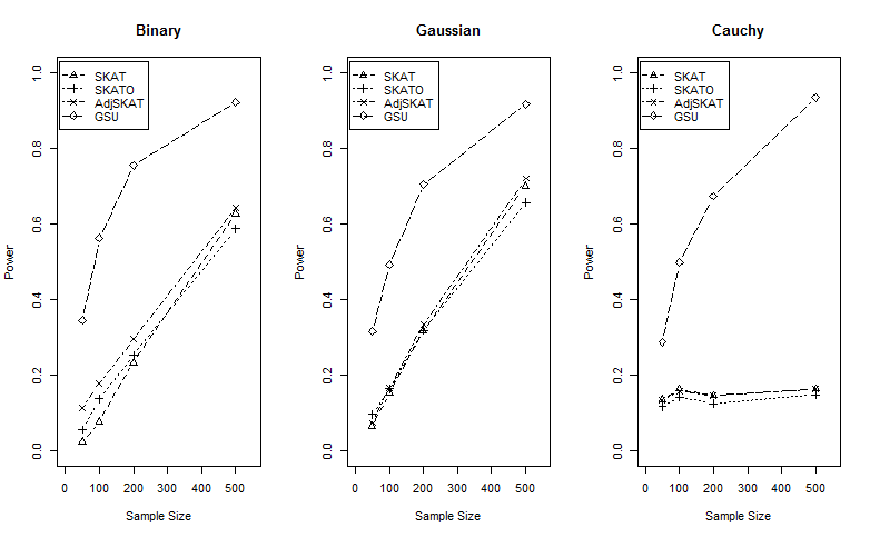
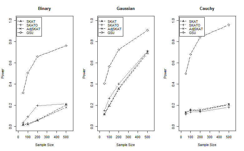
The power comparison is summarized in Figures 1 and 2. For the disease model where half of the causal SNVs were deleterious (Figure 1), GSU had higher power than other methods for various sample sizes ranging from 50 to 500. For instance, in the simulation with binary phenotype and a sample size of 50, GSU (power=0.346) attained much higher power than AdjSKAT (power=0.114), SKATO (power=0.057), and SKAT (power=0.024). Similarly, for the Gaussian-distributed phenotype, GSU had the highest power among the four methods, and the three SKAT-based methods had similar performance. For the Cauchy-distributed phenotype, where the distribution assumption was violated, the power of the SKAT-based methods remained similar as the sample sizes increased, while GSU had increased power as the sample size increased. For the second disease model in which a majority of the SNVs were deleterious (Figure 2), we observed the same conclusion, i.e., GSU had highest power regardless of sample sizes and phenotype distributions.
Intuitively, as a semi-parametric model, SKAT should have comparable power with GSU. The reason for the advantage of GSU lies in the form of test statistics. The score test of SKAT utilizes both diagonal terms and off-diagonal terms of the similarity matrix. When the null model gives the same predicted values (i.e., no covariates), the diagonal terms essentially provide no additional information with regard to association, while adding more variation (i.e., noise) to the score statistic. Meanwhile, GSU utilizes only the off-diagonal terms. When the sample size is small, the influence of diagonal terms will be significant, which is why we observed the higher power of GSU over SKAT. When the sample size becomes larger, the off-diagonal terms will dominate, and the difference of power of two methods becomes smaller.
3.2.2 Result for Simulation II
The type I error rates for the multivariate analysis are summarized in Table 2. Similar to the results of the univariate analysis, GSU can correctly control type I error at the level of 0.05 (Table 2), while the other three methods had inflated type I error when the distribution assumption was violated (e.g., CCC and BGC). When the distribution assumption was satisfied, AdjSKAT correctly controlled the type 1 error. SKAT and SKATO, however, had conservative type I error rates for small sample sizes (50 and 100), especially when the multiple phenotypes comprised of binary-distributed phenotypes (e.g., BBB, BBG and BGG).
| \HlineSample size | Method | Same Distr. 33 3 B, G, and C represent Binary-distributed, Gaussian-distributed, and Cauchy-distributed phenotypes, respectively. | Diff Distr. | ||||
|---|---|---|---|---|---|---|---|
| BBB | GGG | CCC | BBG | BGG | BGC | ||
| 50 | SKAT | 0.002 | 0.028 | 0.232 | 0.008 | 0.021 | 0.097 |
| SKATO | 0.019 | 0.027 | 0.207 | 0.016 | 0.024 | 0.085 | |
| AdjSKAT | 0.046 | 0.028 | 0.237 | 0.049 | 0.040 | 0.113 | |
| GSU | 0.057 | 0.047 | 0.045 | 0.034 | 0.043 | 0.056 | |
| 100 | SKAT | 0.001 | 0.023 | 0.295 | 0.011 | 0.013 | 0.122 |
| SKATO | 0.025 | 0.039 | 0.260 | 0.025 | 0.036 | 0.117 | |
| AdjSKAT | 0.055 | 0.025 | 0.290 | 0.059 | 0.042 | 0.135 | |
| GSU | 0.048 | 0.047 | 0.044 | 0.051 | 0.059 | 0.058 | |
| 200 | SKAT | 0.020 | 0.048 | 0.325 | 0.033 | 0.020 | 0.134 |
| SKATO | 0.030 | 0.058 | 0.288 | 0.035 | 0.036 | 0.118 | |
| AdjSKAT | 0.059 | 0.046 | 0.319 | 0.064 | 0.038 | 0.136 | |
| GSU | 0.050 | 0.047 | 0.049 | 0.058 | 0.056 | 0.043 | |
| 500 | SKAT | 0.044 | 0.035 | 0.364 | 0.035 | 0.04 | 0.166 |
| SKATO | 0.054 | 0.036 | 0.315 | 0.038 | 0.047 | 0.156 | |
| AdjSKAT | 0.06 | 0.038 | 0.342 | 0.041 | 0.049 | 0.172 | |
| GSU | 0.045 | 0.054 | 0.044 | 0.046 | 0.039 | 0.062 | |
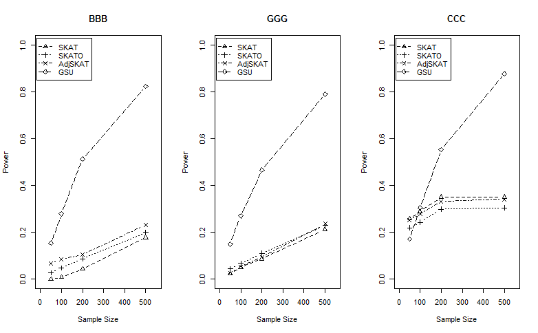
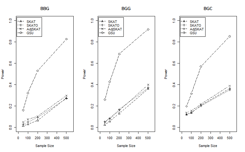
The power comparison of four methods under the two disease models is summerized in Figures 3 and 4. For the disease model where the multiple phenotypes followed the same distribution, GSU had higher power than the three SKAT-based methods (Figure 3). For simulations with BBB phenotypes and GGG phenotypes, GSU attained higher power than the other three methods when the sample size was 50, and obtained substantial power improvement as sample sizes increased. For the simulation with CCC phenotypes, we also observed substantial power improvement of GSU than the other three methods as sample size increased. Yet, the power of the three SKAT-based methods were higher than that of GSU when the sample size was 50. This can be explained by the inflated type 1 error rates of the SKAT-based methods for the Cauchy-distributed phenotypes (Table 2). Similarly, for disease models with a combination of different types of phenotype distribution (i.e., BBG, BGG, and BGC), GSU had higher power than SKAT, SKATO and AdjSKAT, regardless of sample size and phenotype distributions (Figure 4).
Comparing with univariate analysis in simulation I, GSU had further power improvement by considering the association of multi-phenotype in one single test. The three SKAT-based methods, on the other hand, performed multiple univariate analyses with Bonferroni correction. Under the alternative, the multiple phenotypes are correlated to each other. The univariate analysis with Bonferroni correction is subject to power loss without considering the correction structure of multiple phenotypes. Meanwhile, GSU can take the correlation structure into account when constructing the phenotype similarity, and therefore attained higher power than the other three methods.
3.3 Computational Efficiency
We compared the computational efficiency of R-based GSU with SKAT, SKATO and AdjSKAT. We found GSU attained highest computational efficiency among four methods. For example, for the multivariate analysis of BBG phenotype with a sample size of 500 on 1000 simulation replicates, SKAT, SKATO and AdjSKAT took 5 (4320s), 16 (13686s) and 25 (20890s) times longer than GSU (849s), using a personal computer with 2.3GHz CPU and 4G memory. The detailed computational efficiency comparison of four methods for analyzing data with various distributed phenotypes and different sample sizes is given in Table S3 of Supplementary Materials.
Although the comparisons were made under simulation setting, they represent general scenarios in practice. All four methods need to spend substantial time on eigen decomposition in the final step of calculating asymptotic distribution. For multivariate analysis, GSU performs the eigen decomposition once for all phenotypes, while SKAT-based methods need to perform the eigen decomposition for each phenotype. Moreover, if the link function is not identity link, iterative estimation for null model and additional large matrix multiplication and decomposition are required before the final eigen decomposition, which will also increase the computational burden of SKAT-based methods.
4 Application to the Dallas Heart Study
To evaluate the performance of GSU on real data, we applied it to the Dallas Heart Study (DHS) sequence data(Ahituv et al., 2007) and compared the result of GSU with those of three SKAT-based methods. The DHS sequencing data is comprised of 4 genes, ANGPTL3, ANGPTL4, ANGPTL5 and ANGPTL6. After completing the quality control (e.g., removing SNVs with high missing rate), 230 SNVs (54 SNVs, 63 SNVs, 61 SNVs, and 52 SNVs were from ANGPTL3, ANGPTL4, ANGPTL5 and ANGPTL6, respectively) and 2598 subjects remained for the analysis. In the real data analysis, we were interested in testing the association of the SNVs in these genes with multiple metabolic-related phenotypes, including obesity (dichotomized from BMI using a cut-off of 35), cholesterol, high-density lipoprotein cholesterol (HDL), low-density lipoprotein cholesterol (LDL) and very-low-density lipoprotein cholesterol (VLDL).
In order to consider the potential confounding effects of age, gender and race, we adjusted these covariates in the analysis and used the residuals to build phenotype similarity for GSU. Because the three SKAT-based methods cannot directly analyze multiple phenotypes, we obtained smallest p-values from the univariate analysis of all phenotypes and then used the Bonferroni correction to determine whether there was a significant association. The results are summarized in Table 3. Because all 4 genes were metablolic candidate genes, we first combined SNVs in the 4 genes into a single SNV-set. For the joint analysis of 4 genes, GSU could detect a significant association of 4 genes with 4 metabolic-related phenotypes (p-value=0.028), while SKAT, SKATO and AdjSKAT did not detect the association. For further exploration, we analyzed each gene separately and tested its association with 4 metabolic-related phenotypes. By using GSU, we found a marginal association of ANGPTL4 with the multiple phenotypes(p-value=0.057).
| \HlineGene | Rare variants | P-value 44 4 Multiple phenotypes considered in the analysis include BMI, cholesterol, HDL, LDL and VLDL. For SKAT-based methods, each p-value listed in the table is the smallest p-value from 5 univariate analysis, where the Bonferroni corrected significance level should be 0.05/5. | |||
|---|---|---|---|---|---|
| GSU | SKAT | AdjSKAT | SKATO | ||
| ANGPTL3 | 54 | 0.300 | 0.083 | 0.071 | 0.112 |
| ANGPTL4 | 63 | 0.057 | 0.079 | 0.086 | 0.155 |
| ANGPTL5 | 61 | 0.075 | 0.046 | 0.073 | 0.107 |
| ANGPTL6 | 52 | 0.297 | 0.059 | 0.065 | 0.101 |
| ALL | 230 | 0.028 | 0.250 | 0.174 | 0.245 |
5 Discussion
Driven by recent developments in sequencing technologies and the common-diseases-rare-variants hypothesis, sequencing studies are now emerging as a major study design for the genetic association of complex diseases. Yet, the uniqueness of sequencing data, including low MAF and high dimensionality, pose daunting challenges to statistical analysis. The conventional methods, such as a single-locus analysis using logistic regression, had low power for sequencing data analysis. Instead, joint association analysis, or SNV-set analysis, is becoming popular due to its ability to increase power and reduce multiple testing. Although the existing joint association methods have nice features and are easy to use, they also have certain limitations. For example, most of burden tests assume homogeneous effects within the SNV-set, which may not reflect the true underlying disease models. Besides burden tests, most of the existing methods are parametric or semi-perimetric, which often assume certain distributions of the phenotypes and mode of inheritance. When the assumptions are violated, the results can be unreliable.
To overcome these limitations, we have proposed a generalized similarity U test for multivariate analysis of different types of phenotypes. We conducted extensive simulation studies using data from the 1000 Genome Project and compared the performance of GSU with that of three other popular methods: SKAT, AdjSKAT and SKATO. For all of the simulation scenarios, including single phenotype with various distributions, and multiple phenotypes with various combinations of phenotype distribution, GSU outperformed the other three methods in terms of robust type I error and higher power. Although the simulation results depend on the simulation settings, and should always be interpreted in the context of the simulation setting, we believe the results reflect the advantage of GSU in a broader sense, because 1) the genetic data used in the simulation comes from the 1000 Genome Project, which reflects the LD pattern and the allelic frequency distribution in the general population; and 2) we simulated a wide range of disease models to mimic common disease scenarios.
In recent years, U-statistic-based methods have been popularly used in genetic data analysis, and have shown their robustness and flexibility for analyzing genetic data(Schaid et al., 2005; Zhang et al., 2010; Wei et al., 2013). GSU is a general framework based on similarity measurements. Although in this paper we used the weighted-IBS to calculate genetic similarity, other forms of genetic similarity can also be used. For the weighted-IBS similarity, we can modify the weights (i.e., the original weight ) to reflect the importance of each SNV. Besides IBS-based similarity, we can also use distance-transformed similarity to model the effect in a nonlinear way. For example, we can use the Euclidean-Distance-based similarity, . In this paper, we have focused on the analysis of categorical sequencing data (i.e, SNV data). By using appropriate genetic similarity measurements, GSU can easily be extended to analyze other types of genetic data, such as count data (CNV data) and continuous data (expression data).
The flexibility of GSU also comes from the construction of the phenotype similarity. By using phenotype similarity, GSU can analyze not only a single phenotype, but also multiple phenotypes following different distributions. Many genetic studies collect multiple secondary phenotypes, or use intermediate biomarkers, to study complex diseases. By considering multiple phenotypes that measure the different aspects of underlying diseases, the power of association analysis can be potentially improved (Zhang et al., 2010; Liu et al., 2009; Maity et al., 2012). Nevertheless, few methods have been developed for multivariate analysis of sequencing data. Methods were recently developed for multivariate analysis of common genetic variants, but relies on the normal assumption for the phenotype distribution (Maity et al., 2012). GSU is developed for both univariate and multivariate analysis of sequencing data. It is distribution-free and can analyze multiple phenotypes with a combination of different types of phenotype. Nevertheless, similar as all other non-parametric tests, it is not straightforward for GSU to perform covariate adjustment. One possible solution is to adopt the idea of covariate adjustment in regression, and include covariates when we calculate the centered similarity (e.g., ).
Supplementary Materials
Supplementary Materials are available with this paper at the Biometrics website on Wiley Online Library.
References
- Abecasis et al. (2010) Abecasis, G. R., Altshuler, D., Auton, A., Brooks, L. D., Durbin, R. M., Gibbs, R. A., Hurles, M. E., and McVean, G. A. (2010). A map of human genome variation from population-scale sequencing. Nature 467, 1061–73.
- Ahituv et al. (2007) Ahituv, N., Kavaslar, N., Schackwitz, W., Ustaszewska, A., Martin, J., Hebert, S., Doelle, H., Ersoy, B., Kryukov, G., Schmidt, S., Yosef, N., Ruppin, E., Sharan, R., Vaisse, C., Sunyaev, S., Dent, R., Cohen, J., McPherson, R., and Pennacchio, L. A. (2007). Medical sequencing at the extremes of human body mass. American Journal of Human Genetics 80, 779–791.
- Boyko et al. (2008) Boyko, A. R., Williamson, S. H., Indap, A. R., Degenhardt, J. D., Hernandez, R. D., Lohmueller, K. E., Adams, M. D., Schmidt, S., Sninsky, J. J., Sunyaev, S. R., White, T. J., Nielsen, R., Clark, A. G., and Bustamante, C. D. (2008). Assessing the evolutionary impact of amino acid mutations in the human genome. Plos Genetics 4,.
- Cohen et al. (2004) Cohen, J. C., Kiss, R. S., Pertsemlidis, A., Marcel, Y. L., McPherson, R., and Hobbs, H. H. (2004). Multiple rare alleles contribute to low plasma levels of hdl cholesterol. Science 305, 869–872.
- Davies (1980) Davies, R. B. (1980). Algorithm as 155: The distribution of a linear combination of x2 random variables. Journal of the Royal Statistical Society. Series C (Applied Statistics) 29, 323–333.
- Dick and Agrawal (2008) Dick, D. M. and Agrawal, A. (2008). The genetics of alcohol and other drug dependence. Alcohol Research & Health 31, 111.
- Fay et al. (2001) Fay, J. C., Wyckoff, G. J., and Wu, C. I. (2001). Positive and negative selection on the human genome. Genetics 158, 1227–1234.
- Gregory (1977) Gregory, G. G. (1977). Large sample theory for u-statistics and tests of fit. Annals of Statistics 5, 110–123.
- Ji et al. (2008) Ji, W. Z., Foo, J. N., O’Roak, B. J., Zhao, H., Larson, M. G., Simon, D. B., Newton-Cheh, C., State, M. W., Levy, D., and Lifton, R. P. (2008). Rare independent mutations in renal salt handling genes contribute to blood pressure variation. Nature Genetics 40, 592–599.
- Kryukov et al. (2007) Kryukov, G. V., Pennacchio, L. A., and Sunyaev, S. R. (2007). Most rare missense alleles are deleterious in humans: Implications for complex disease and association studies. American Journal of Human Genetics 80, 727–739.
- Kuonen (1999) Kuonen, D. (1999). Saddlepoint approximations for distributions of quadratic forms in normal variables. Biometrika 86, 929–935.
- Lee et al. (2012) Lee, S., Emond, M. J., Bamshad, M. J., Barnes, K. C., Rieder, M. J., Nickerson, D. A., Christiani, D. C., Wurfel, M. M., and Lin, X. H. (2012). Optimal unified approach for rare-variant association testing with application to small-sample case-control whole-exome sequencing studies. American Journal of Human Genetics 91, 224–237.
- Li and Leal (2008) Li, B. S. and Leal, S. M. (2008). Methods for detecting associations with rare variants for common diseases: Application to analysis of sequence data. American Journal of Human Genetics 83, 311–321.
- Lin and Tang (2011) Lin, D.-Y. and Tang, Z.-Z. (2011). A general framework for detecting disease associations with rare variants in sequencing studies. American journal of human genetics 89, 354–367.
- Lindsay et al. (2008) Lindsay, B. G., Markatou, M., Ray, S., Yang, K., and Chen, S. C. (2008). Quadratic distances on probabilities: A unified foundation. Annals of Statistics 36, 983–1006.
- Liu et al. (2009) Liu, H., Tang, Y. Q., and Zhang, H. H. (2009). A new chi-square approximation to the distribution of non-negative definite quadratic forms in non-central normal variables. Computational Statistics & Data Analysis 53, 853–856.
- Liu et al. (2009) Liu, J., Pei, Y., Papasian, C. J., and Deng, H.-W. (2009). Bivariate association analyses for the mixture of continuous and binary traits with the use of extended generalized estimating equations. Genetic Epidemiology 33, 217–227.
- Luo et al. (2012) Luo, L., Zhu, Y., and Xiong, M. (2012). Quantitative trait locus analysis for next-generation sequencing with the functional linear models. Journal of Medical Genetics 49, 513–524.
- Lynch and Ritland (1999) Lynch, M. and Ritland, K. (1999). Estimation of pairwise relatedness with molecular markers. Genetics 152, 1753–1766.
- Madsen and Browning (2009) Madsen, B. E. and Browning, S. R. (2009). A groupwise association test for rare mutations using a weighted sum statistic. Plos Genetics 5,.
- Maity et al. (2012) Maity, A., Sullivan, P. E., and Tzeng, J. Y. (2012). Multivariate phenotype association analysis by marker-set kernel machine regression. Genetic Epidemiology 36, 686–695.
- Morgenthaler and Thilly (2007) Morgenthaler, S. and Thilly, W. G. (2007). A strategy to discover genes that carry multi-allelic or mono-allelic risk for common diseases: A cohort allelic sums test (cast). Mutation Research-Fundamental and Molecular Mechanisms of Mutagenesis 615, 28–56.
- Neale et al. (2011) Neale, B. M., Rivas, M. A., Voight, B. F., Altshuler, D., Devlin, B., Orho-Melander, M., Kathiresan, S., Purcell, S. M., Roeder, K., and Daly, M. J. (2011). Testing for an unusual distribution of rare variants. Plos Genetics 7,.
- O’Neil and Redner (1993) O’Neil, K. A. and Redner, R. A. (1993). Asymptotic distributions of weighted u-statistics of degree 2. The Annals of Probability 21, 1159–1169.
- Pritchard (2001) Pritchard, J. K. (2001). Are rare variants responsible for susceptibility to complex diseases? American Journal of Human Genetics 69, 124–137.
- Romeo et al. (2009) Romeo, S., Yin, W., Kozlitina, J., Pennacchio, L. A., Boerwinkle, E., Hobbs, H. H., and Cohen, J. C. (2009). Rare loss-of-function mutations in angptl family members contribute to plasma triglyceride levels in humans. Journal of Clinical Investigation 119, 70–79.
- Schaid et al. (2005) Schaid, D. J., McDonnell, S. K., Hebbring, S. J., Cunningham, J. M., and Thibodeau, S. N. (2005). Nonparametric tests of association of multiple genes with human disease. American Journal of Human Genetics 76, 780–793.
- Shapiro and Hubert (1979) Shapiro, C. P. and Hubert, L. (1979). Asymptotic normality of permutation statistics derived from weighted sums of bivariate functions. The Annals of Statistics 7, 788–794.
- Shieh (1997) Shieh, G. S. (1997). Weighted degenerate u- and v-statistics with estimated parameters. Statistica Sinica 7, 1021–1038.
- Tzeng et al. (2009) Tzeng, J.-Y., Zhang, D., Chang, S.-M., Thomas, D. C., and Davidian, M. (2009). Gene-trait similarity regression for multimarker-based association analysis. Biometrics 65, 822–832.
- van der Vaart and Wellner (2000) van der Vaart, A. and Wellner, J. A. (2000). weak convergence and empirical processes. Springer, 2 edition.
- Wei et al. (2013) Wei, C. S., Schaid, D. J., and Lu, Q. (2013). Trees assembling mann-whitney approach for detecting genome-wide joint association among low-marginal-effect loci. Genetic Epidemiology 37, 84–91.
- Wu et al. (2011) Wu, M. C., Lee, S., Cai, T. X., Li, Y., Boehnke, M., and Lin, X. H. (2011). Rare-variant association testing for sequencing data with the sequence kernel association test. American Journal of Human Genetics 89, 82–93.
- Zhang et al. (2010) Zhang, H. P., Liu, C. T., and Wang, X. Q. (2010). An association test for multiple traits based on the generalized kendall’s tau. Journal of the American Statistical Association 105, 473–481.
Appendix A: Centered Similarity
By the following definition of centered similarity,
we can obtain conditional expectation for the centered phenotype similarity,
Therefore, we have and . Using the same argument, we can have the same result for the centered genetic similarity.
Under the null hypothesis, when the genetic similarities are independent of the phenotype similarities, we have,
Appendix B: Proof of Theorem 1
We can decompose the centered phenotype similarity by,
where and are eigenvalues and eigenfunctions of the kennel .
Because of the orthogonality of , we have
We showed in Appendix A, which forced and to be an eigenfunction-eigenvalue pair in the decomposition of . Again, because is orthogonal with , for , we have
Using the same argument, we have the corresponding results for the decomposition of the centered genetic similarity:
Then,
| (Ax.1) |
Using the function decomposition, we can write GSU as,
where and .
Under the null hypothesis, genotype () is independent of phenotypes (). Therefore, for and ,
| (Ax.2) |
and
| (Ax.3) |
Therefore, for any finite subset of , converges to a multivariate normal distribution by using results from equation Ax.2, equation Ax.3 and multivariate CLT.
Additionally, we can show that,
Under the condition , the countable sequence of function is a Donsker class(van der Vaart and Wellner, 2000). Therefore, the empirical process, , converges weakly to the Gaussian process with mean zero and covariance function,
With this uniform convergence (for all and ), we can show that,
where are i.i.d chi-squared random variables with a d.f. of 1.
Appendix C: Proof of Theorm 2
To simplify the notation, we denote and . GSU can then be rewritten as:
Define a centered kernel by:
where .
We can decompose the GSU as follows:
Thus,
Becuase and , the first term converges to normal distribution by applying CLT:
Then we need to show:
This can be done by proving , using the fact that , and . In fact, by using the similar technique in Appendix C, we can show that asymptotically follows the distribution of a weighted sum of independent chi-square random variables.
Appendix D: Matrix Similarity
In the study sample, we can calculate the centered phenotype similarity by:
Denote and , the above equation becomes:
The equations can be written in a matrix form,
where , , , and .
Similarly, the centered genetic similarity can also be written in the matrix form:
where , and .
Appendix E: Limiting Distribution
In the actual computation, we will use a matrix eigen-decomposition to obtain the eigenvectors as a finite-dimension approximation of the eigenfunctions. For a matrix eigen-decomposition, a computer algorithm usually gives the eigenvalue with the eigenvector , which satisfies instead of . Therefore, using the eigenvalues and calculated from the matrix eigen-decomposition, the limiting distribution of GSU is:
.