Generalized Yule-Walker Estimation for Spatio-Temporal
Models
with Unknown Diagonal Coefficients
Abstract
We consider a class of spatio-temporal models which extend popular econometric spatial autoregressive panel data models by allowing the scalar coefficients for each location (or panel) different from each other. To overcome the innate endogeneity, we propose a generalized Yule-Walker estimation method which applies the least squares estimation to a Yule-Walker equation. The asymptotic theory is developed under the setting that both the sample size and the number of locations (or panels) tend to infinity under a general setting for stationary and -mixing processes, which includes spatial autoregressive panel data models driven by innovations as special cases. The proposed methods are illustrated using both simulated and real data.
JEL classification: C13, C23, C32.
Keywords: -mixing, Dynamic panels, High dimensionality, Least squares estimation, Spatial autoregression, Stationarity.
1 Introduction
The class of spatial autoregressive (SAR) models is introduced to model cross sectional dependence of different economic individuals at different locations (Cliff and Ord, 1973). More recent developments extend SAR models to spatial dynamic panel data (SDPD) models, i.e. adding time lagged terms to account for serial correlations across different locations. See, e.g. Lee and Yu (2010a). Baltagi et al. (2003) considers a static spatial panel model where the error term is a SAR model. Lin and Lee (2010) shows that in the presence of heteroskedastic disturbances, the maximum likelihood estimator for the SAR models without taking into account the heteroskedasticity is generally inconsistent and proposes an alternative GMM estimation method. Computationally the GMM methods are more efficient than the QML estimation (Lee, 2001). Lee and Yu (2010a) classifies SDPD models into three categories: stable, spatial cointegration and explosive cases. As pointed out by Bai and Shi (2011), the cases with a large number of cross sectional units and a long history are rare. Hence it is pertinent to consider the setting with short time spans in order to include as many locations as possible. Both estimation method and asymptotic analysis need to be adapted under this new setting. Yu et al. (2008) and Yu et al. (2012) investigate the asymptotic properties when both the number of locations and the length of time series tend to infinity for both the stable case and spatial cointegration case, and show that QMLE is consistent.
Motivated by the evidence in some practical examples, we extend the model in Yu et al. (2008) and Yu et al. (2012) by allowing the scalar coefficients for each location (or panel) different from each other. This increase in model capacity comes with the cost of estimating substantially more parameters. In fact that the number of the parameters in this new setting is in the order of the number of locations. The model considered in this paper has four additive components: a pure spatial effect, a pure dynamic effect, a time-lagged spatial effect and a white noise. Due to the innate endogeneity, the conventional regression estimation methods such as the least squares method directly based on the model lead to inconsistent estimators. To overcome the difficulties caused by the endogeneity, we propose a generalized Yule-Walker type estimator for estimating the parameters in the model, which applies the least squares estimation to a Yule-Walker equation. The asymptotic normality of the proposed estimators is established under the setting that both the sample size and the number of locations (or panels) tend to infinity. Therefore the number of parameters to be estimated also diverges to infinity, which is a marked difference from, e.g., Yu et al. (2012). We develop the asymptotic properties under a general setting for stationary and -mixing processes, which includes the spatial autoregressive panel data models driven by innovations as special cases.
The rest of the paper is organized as follows. Section 2 introduces the new model, its motivation and the generalized Yule-Walker estimation method. The asymptotic theory for the proposed estimation method is presented in Section 3. Simulation results and real data analysis are reported, respectively, in Section 4 and 5. All the technical proofs are relegated to an Appendix.
2 Model and Estimation Method
2.1 Models
The model considered in this paper is of the following form:
| (1) |
where represents the observations from locations at time , and is the unknown coefficient parameter for the -th location, and is the spatial weight matrix which measures the dependence among different locations. All the main diagonal elements of are zero. It is a common practice in spatial econometrics to assume known. For example, we may let , for , where is an appropriate distance between the -th and the -th location. It can simply be the geographical distance between the two locations or the distance reflecting the correlation or association between the variables at the two locations. In the above model, captures the pure spatial effect, captures the pure dynamic effect, and captures the time-lagged spatial effect. We also assume that the error term in (1) satisfies the condition When for , (1) reduces to the model of Yu et al. (2008), in which there are only 3 unknown regressive coefficient parameters. In general the regression function in (1) contains unknown parameters.
The extension to use different scalar coefficients for different locations is motivated by practical needs. For example, we analyze the monthly change rates of the consumer price index (CPI) for the EU member states over the years 2003-2010. The detailed analysis for this data set will be presented in section 5. Figure 1 presents the scatter-plots of the observed data versus the spatial regressor and , for some of the EU member states, where is the -th row vector of the weight matrix which is taken as the sample correlation matrix with all the elements on the main diagonal set to be 0. The superimposed straight lines are the simple regression lines estimated using the newly proposed method in Section 2.2 below. It is clear from Figure 1 that at least Greece and Belgium should have a different slope from those of France or Iceland.


2.2 Generalized Yule-Walker estimation
As occurs on both sides of (1), and are correlated with each other. Applying least squares method directly based on regressing on leads to inconsistent estimators. On the other hand, applying the maximum likelihood estimation requires to profile a nuisance parameter matrix , which leads to a complex nonlinear optimization problem. Furthermore when is large in relation to , the numerical stability is of concern.
We propose below a new estimation method which applies the least squares method to each individual row of a Yule-Walker equation. To this end, let for any . Note that we always assume that is stationary, see condition A2 and Remark 1 in Section 3 below. Then the Yule-Walker equation below follows from (1) directly.
where is a identity matrix. The -th row of the above equation is
| (2) |
where is the -th row vector of , and is the unit vector with the -th element equal to 1. Note that (2) is a system of linear equations with three unknown parameters , and . Since , we replace and by the sample (auto)covariance matrices
We estimate by the least squares method, i.e. to solve the minimization problem
The resulting estimators are called generalized Yule-Walker estimators which admits the explicit expression:
| (3) |
where
More explicitly,
Then it holds that for ,
2.3 A root- consistent estimator for large
When , the estimator (3) admits non-standard convergence rates (i.e. the rates different from ); see Theorems 2 and 4 in Section 3 below. Note that there are equations with only 3 parameters in (2). Hence (3) can be viewed as a GMME for an over-determined scenario. The estimation may suffer when the number of estimation equations increases. See, for example, a similar result in Theorem 1 of Chang, Chen and Chen (2015). A further compounding factor is that the estimation for the covariance matrices using their sample counterparts leads to non-negligible errors even when . Below we propose an alternative estimator which restricts the number of the estimation equations to be used in order to restore the -consistency and the asymptotic normality.
For , put Note that the -th row of is which is the covariance between and . Let
| (4) |
Then may be viewed as a measure for the correlation between and . When is small, say, close to 0, the -th equation in (2) carries little information on . Therefore as far as the estimation for is concerned, we only keep the -th equation in (2) for large .
Let be the vector consisting of those corresponding to the largest (), where is defined as in (4) but with replaced by . The new estimator is defined as
| (5) |
where
| (6) |
and
Now it holds that
Theorem 3 in Section 3 below shows the asymptotic normality of the above estimator provided that the number of estimation equations used satisfies condition .
3 Theoretical properties
We introduce some notations first. For a vector , is the Euclidean norm, is the norm. For a matrix , is the Frobenius norm, is the operator norm, where is the largest eigenvalue of a matrix. We denote by the matrix which is a matrix of the same size as but with the -th element replaced by . Note the determinant of is denoted by . A strictly stationary process is -mixing if
| (7) |
where denotes the -algebra generated by . See, e.g., Section 2.6 of Fan and Yao (2003) for a compact review of -mixing processes.
Let be invertible. It follows from (1) that
where . Some regularity conditions are now in order.
- A1.
The spatial weight matrix is known with zero main diagonal elements; is invertible.
- A2.
- A3.
The rank of matrix is equal to 3.
Remark 1. Condition A1 is standard for spatial econometric models. Condition A3 ensures that and are identifiable in (2). Condition A2(c) limits the dependence across different spatial locations. It is implied by, for example, the conditions imposed in Yu et al. (2008). Lemma 1 in the Appendix shows that Condition A2 holds with under conditions A1 and B1 – B3 below. Note that conditions B1–B3 are often directly imposed in the spatial econometrics literature including, for example, Lee and Yu (2010a), and Yu et al. (2008).
- B1.
The errors are across and with , , and . The density function of exists.
- B2.
The row and column sums of and are bounded uniformly in .
- B3.
The row and column sums of are bounded uniformly in .
Now we are ready to present the asymptotic properties for , , with fixed and first, and then and .
3.1 Asymptotics for fixed
For , let
| (8) |
and
| (9) |
Theorem 1
Let conditions A1 – A3 hold and be fixed. Then as , it holds that
where and are given in and .
3.2 Asymptotics with diverging
When diverges together with , in (9) and (8) are no longer constant matrices. Let be a matrix such that .
Theorem 2
Let condition A1 – A3 hold.
- (i)
As , and ,
- (ii)
As , , and ,
Theorem 2 indicates that the standard root- convergence rate prevails as long as . However the convergence rate may be slower when is of higher orders than . Theorem 2 presents the convergence rates for the norm of the estimation errors. The rates also hold for the norm of the errors as well. Corollary 1 consider the estimation errors over locations together, for which we have established the result for norm only.
Corollary 1
Let condition A1 hold, and condition A2 and A3 hold for all . Then as and , it holds that
To derive the asymptotic properties of the estimators defined in (5), we introduce some new notation. For , let
and
Let
| (10) |
and
| (11) |
Theorem 3 below indicates that the estimators defined in (5) are asymptotically normal with the standard -rate as long as . Note that it does not impose any conditions directly on the size of .
- A4.
Theorem 3
Let conditions A1, A2(a,b) and A4 hold. As , and , it holds that
where and are given in and .
The key assumption of Theorem 2 is A2(c), which decides the fact that the effect of the dimensionality only comes from in equation (13) in the Appendix. We can relax this assumption by allowing to be affected by as well. Under the new relaxed assumption, we may obtain a better convergent rate of estimator (3) by making use of the fact that (3) is invariant if we divide both the numerator and denominator by the same number, for example, a number relating to . This will be presented in Theorem 4. We propose the new relaxed assumption:
- A5.
For specified in A2(b),
and the diagonal elements of defined in (8) is in the order of , where , and are numbers relating to .
Denote as a constant. When the number of nonzero elements (or elements bounded away from zero) in increases with but is , we may have . Simulation scenario 2 is under this case. When there are only finite number of nonzero elements (or elements bounded away from zero) in , we might have , which is the case of simulation scenario 1. The reason we assume the diagonal elements of defined in (8) are in the order of is because we can treat as the second moments of three random variables and respectively, where the random vector has mean 0 and covariance matrix .
Theorem 4
Let conditions A1, A2(a,b), A3 and A5 hold. As , , if and , it holds that
Let us consider some examples. (1) When , and , the convergence rate is . (2) When , and , if , the convergence rate is . (3) When , and , if , the convergence rate is , which corresponds with Theorem 2. Theorem 4 indicates that under different situations of , and , we may obtain different convergence rates. These observations are illustrated by simulation examples in section 4.
4 Simulation study
To examine the finite sample performance of the proposed estimation methods, we conduct some simulation under different scenarios.
4.1 Scenario 1
, and are generated from . The spatial weight matrix used is a block diagonal matrix formed by a row-normalized matrix . We construct such that the first four sub-diagonal elements are all 1 and the rest elements are all 0 before normalizing. This kind of corresponds to the pooling of separate districts with similar neighboring structures in each district, see Lee and Yu (2013). The error are independently generated from , where we generate each from .
For all scenarios, we generate data from (2.1) with different settings for and . We apply the proposed estimation method (2.3) and (2.5) (with ) and report the mean absolute errors:
We replicate each setting 500 times.
Figure 2 depicts two boxplots of MAE with equals to, respectively, 25 and 100. As the sample size increases from 100, 250, 500, 750 to 1000, MAE decreases for both methods.

Figure 3 depicts the boxplots of the MAE for the original estimator (2.3), the root consistent estimator (2.5), and the estimator (2.5) with the ridge penalty, where we choose the ridge tuning parameter to be in order to avoid the nearly singularity problem of , and is chosen via cross validation. With , the dimension is set at 25,49,64,81,100,169,324 and 529 respectively. The MAE for (2.3) remains about the same level as increases; see the panel on the left in Figure 3. This is in line with the asymptotic result of Theorem 4 when, for example, , and . In contrast, the MAE for estimator (2.5) increases sharply when increases; see the panel in the middle. This is due to the fact that is nearly singular for large . Adding a ridge in the estimator certainly mitigates the deterioration when increases; see the panel on the right in Figure 3.

4.2 Scenario 2
, and are generated from . The spatial weight matrix is constructed as follows. First, we construct a row-normalized matrix , where is chosen such that the first two sub-diagonal elements are all 1 and the rest elements are all 0 before normalizing. Then we treat as a block matrix and put into the main diagonal, 2nd, 4th, 6th and etc. sub-diagonal block positions. This kind of corresponds to the pooling of districts (each district has locations) which the evenly numbered districts are connected and the oddly numbered districts are connected but evenly numbered districts and oddly number districts are separated. Each district has similar neighboring structures. As increases, the number of the locations influencing one specific location increases in the order of . The error are independently generated from , where we generate each from .
Figure 4 depicts two boxplots of MAE with equals to, respectively, 25 and 100. As the sample size increases from 100, 250, 500, 750 to 1000, MAE decreases for both methods.

Figure 5 depicts three boxplots as Figure 3. The MAE for (2.3) increases steadily as increases, which matches the result of Theorem 4 when, for instance, , and . The MAE for (2.5) after adding ridge penalty is slowly increasing as well. This might be caused by the fact that, similar to A2(c), quantities in condition A4(a) is also influenced by since the number of nonzero elements in is in the order of .

5 Real data analysis
5.1 European Consumer Price Indices
We analyze the monthly change rates of the consumer price index (CPI) for the EU member states, over the years 2003-2010. We use the national harmonized index of consumer prices calculated by Eurostat, the statistical office of the European Union. For this data set, and .
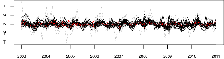
Figure 6 presents the time series plots of the monthly change rates of CPI for the 31 states. To line up the curves together, each series is centered at its mean value in Figure 6. There exist clearly synchronizes on the fluctuations across different states, indicating the spatial (i.e. cross-state) correlations among different states. Also noticeable is the varying degrees of the fluctuation over the different states.
Let consist of the monthly change rates of CPI for the 31 states. We fit the proposed spatial-temporal model (1) to this data set with the parameters estimated by (3). We take a normalized sample correlation matrix of as the spatial weight matrix , i.e. we let be the absolute value of the sample correlation between the -th and -th states for , and , and then replace by .
Figure 7 presents the scatter plots of against, respectively, the 3 regressors in model (1), i.e. , for four selected states Belgium, Greece, France and Iceland. We superimpose the straight line in each of those 3 scatter plots with, respectively, . It is clear that the estimated slopes are very different for those 4 states. Figure 8 plots the true monthly change rates of the CPI for those 4 states together with the fitted values
| (12) |


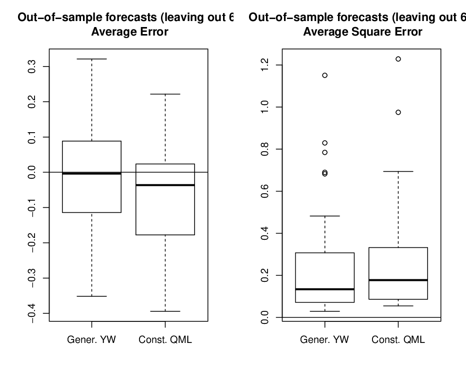
Overall tracks its truth value reasonably well. Figure 9 shows the out-of-sample forecasting performance of our model. For the sake of comparison, predictions are made using our model and the proposed generalized Yule-Walker estimator, and using the (constant) SDPD model of Yu et al. (2008) and their Quasi-Maximum Likelihood estimator. In particular, for each location, we leave out from the sample the last six observations and we compute the (out-of-sample) forecasts with 1,2,….6 step ahead forecasting horizon; then, we compute the average prediction error over time (i.e. the mean of the 6 prediction errors). On the left panel of Figure 9, the two box-plots summarize the average prediction error for the 31 locations obtained with our YW estimator and the QML estimator of Yu et al. (2008), respectively. It is evident that our estimator produces unbiased predictions while the QML estimator appears to be biased. This advantage also reflects on the forecasting average square errors, reported on the right panel of Figure 9. In conclusion, the SDPD model of Yu et al. (2008) has a satisfying forecasting performance because several locations have similar spatial structure and for those locations a model with constant parameters is sufficient. Anyway, a marginal improvement is observed for our estimator because several locations have quite different structures and our model is able to capture this difference. Finally, it is worthwhile to notice that the variability of the two predictors appears to be the same.


To further vindicate the necessity to use different coefficients for different states, we consider a statistical test for hypothesis
for model (1). Then the residuals resulting from the fitted model under will be greater than the residuals without . However if is true, the difference between the two sets of residuals should not be significant. We apply a bootstrap method to test this significance. Let be the estimates under hypothesis . Define the test statistic
We reject for large values of . To assess how large is large, we generate a bootstrap data from
where are drawn independently from the residuals
and consists of the components defined in (12). Now the bootstrap statistic is defined as
where is the estimated coefficients for the regression model
The -value for testing hypothesis is defined as
which is approximated by the relative frequency of the event in a repeated bootstrap sampling with a large number of replications. By repeating bootstrap sampling 1000 times, the estimated -value is 0, exhibiting strong evidence against the null hypothesis . Therefore the model with the equal slope parameters across different locations is inadequate for this particular data set.
5.2 Modeling mortality rates
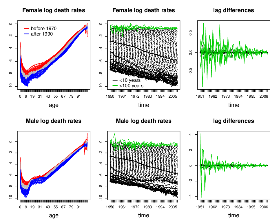
Now we analyze the annual Italian male and female mortality rates for different ages (between 0 and 104) in the period of 1950 – 2009 based on the proposed model (1). The data were downloaded from the Human Mortality Database (see the website http://www.mortality.org/). Let be the log mortality rate of female or male at age and in Year . Those data are plotted in Figure 10. Two panels on the left plot are the female and male mortality against different age in each year. More precisely the curves for are plotted in red, those for are in blue, those with are in grey. Those curves show clearly that the mortality rate decreases over the years for almost all age groups (except a few outliers at the top end). Two panels in the middle of Figure 10 plot the log mortality for each age group against time with the following color code: black for ages not great than 10, grey for ages between 11 and 100, and green for ages greater than 100. They indicate that the mortality for all age groups decreases over time, the most significant decreases occur at the young age groups. Furthermore, the fluctuation of the mortality rates for the top age groups reduces significantly over the years, while the mean mortality rates for those groups remain about the same. This can be seen more clearly in the two panels on the right which plot differenced log mortality rates , using the same colour code, where
We fit the differenced log mortality data with model (1) with the parameters estimated by (5) and . Note that now and . Let the off-diagonal elements of the spatial weight matrix be
We then replace by . Moreover, we can also fix a threshold and set to zero all the elements of matrix such that (for simplicity, we fix in this application, but the results are substantially invariant for different values of ).
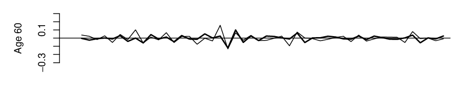
The results of the estimation are shown in table 1, for a selection of cohorts of different ages. Figure 11 shows the fitted series for ages .
| age | age | ||||||
|---|---|---|---|---|---|---|---|
| 5 | 0.41 | -0.52 | 0.06 | 55 | 0.19 | -0.88 | 0.28 |
| 10 | 0.20 | -0.42 | 0.05 | 60 | -0.09 | -0.72 | 0.01 |
| 15 | 0.44 | -0.65 | 0.18 | 65 | 0.22 | -0.63 | 0.21 |
| 20 | 0.64 | -0.78 | 0.40 | 70 | 0.21 | -0.69 | 0.08 |
| 25 | -0.04 | -0.43 | 0.03 | 75 | 0.33 | -0.59 | 0.22 |
| 30 | 0.78 | -0.80 | 0.55 | 80 | 0.33 | -0.89 | 0.27 |
| 35 | 0.11 | -0.55 | 0.29 | 85 | 0.37 | -0.76 | 0.18 |
| 40 | -0.04 | -0.66 | -0.01 | 90 | 0.29 | -0.62 | 0.16 |
| 45 | 0.29 | -0.46 | 0.12 | 95 | 0.27 | -0.77 | 0.26 |
| 50 | -0.10 | -0.45 | -0.05 | 100 | 0.44 | -0.69 | -0.03 |
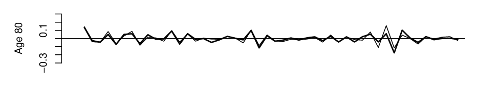
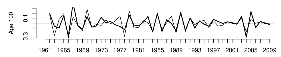
6 Final remark
We propose in this paper a generalized Yule-Walker estimation method for spatio-temporal models with diagonal coefficients. The setting enlarges the capacity of the popular spatial dynamic panel data models. Both the asymptotic results and numerical illustration show that the proposed estimation method works well, although the number of the estimation equations utilized should be of the order .
Appendix: Proofs
We present the proofs for Theorems 2, Corollary 1 and Theorem 4 in this appendix. The proofs for Theorem 1 and 3 are similar and simpler than that of Theorem 2, and they are therefore omitted. We also present a lemma (i.e. Lemma 1) at the end of this appendix, which shows that condition A2 is implied by conditions A1 and B1 – B3; see Remark 1. We use to denote a generic positive constant, which may be different at different places.
Proof of Theorem 2. We first prove (i) of Theorem 2. We only need to prove the assertions (1) and (2) below, as then the required conclusion follows from (1) and (2) immediately.
- (1)
- (2)
To prove (1), it suffices to show that for any nonzero vector , the linear combination
is asymptotic normal.
Let us take out the dominant term in first.
| (13) |
For term and , by Proposition 2.5 of Fan and Yao (2003), we have
| (14) |
where is independent of . Then it holds that
Therefore
Similarly,
Since , it holds that . Similar to (14), we have . Given , it holds that . Hence if ,
Similarly, given , we have
Now it suffices to prove
is asymptotic normal.
Note that it holds that
Now we calculate the variance of . It holds that
| (15) |
and it follows from that
Similarly,
and . Calculating all the variance and covariance and summing up them, it follows from dominate convergence theorem that
To prove the asymptotic normality of , we employ the small-block and large-block arguments. We partition the set into subsets with large blocks of size , small blocks of size and the last remaining set of size . Put
where . Hence
Note that is important when we derive the Lindeberg condition of the truncated partial sum defined in (16).
Since , we have . It then holds that
Then we can partition in the following way
where
Note that and , , by applying proposition 2.7 of Fan and Yao (2003), it holds that
Therefore
We calculate the variance of . Similar to (15), it holds that
Calculating all the variance and covariance and summing up them, by dominated convergence theorem and , it holds that
Now it suffices to prove the asymptotic normality of . We partition into two parts via truncation. Specifically, we define
and
Similarly, we have and . Then
| (16) |
Similar to computing the , it holds that
where is the sum of all the rest variance and covariance except . Therefore
where we denote as the asymptotic variance of . Similarly, we have
Define
where now. We bound as follows
Following the same arguments as part 2.7.7 of Fan and Yao (2003), for any , it holds that as . Hence
Substituting by , it holds that
which leads to the fact that
To prove (2), let us look at the -th element of . We have
| (17) |
Using the same arguments as (14), the first term is and the second term is . Hence given , it holds that
Applying the same arguments to the other elements of , it holds that
To prove (ii) in Theorem 2, the required asymptotic result follows from (13) and (17) immediately when and . The proof is completed.
Proof of Corollary 1. By Theorem 2, it holds that
for all . The required asymptotic result follows from the above result directly.
Proof of Theorem 4. Let us look at term and in (13) first under the new condition (A5). Similar to the proof of (14), it holds that
Hence
Similarly, we have
For the first diagonal element of , it follows from considering the three terms in (17) separately that
Similarly,
Given and , we have
Divide both the numerator and denominator of estimator (3) by , it holds that
The required result then follows directly.
Lemma 1
Under conditions A1 and B1 – B3, condition A2 holds with .
Proof. It is apparent that part (a) of A2 is satisfied under A1 and B1 – B3. is strictly stationary because are across and and condition B3. Since the density function of exists, decays exponentially fast, see Pham and Tran (1985). Therefore . Now we prove A2(c) when .
We present a more general result first: for any vector satisfying , it holds that
Note that
Then
| (18) |
And
| (19) |
where is the -th element of the column vector .
Since where the row and column sums of are bounded uniformly in , it holds that the row and column sums of are bounded uniformly in . Note that
where the row and column sums of and are bounded uniformly in . Hence the row and column sums of are bounded uniformly in . It follows from (18) and (19) that
It is easy to prove that
Thus and etc.
The row and column sums of and are bounded uniformly in . Then
Similarly, we can prove the other diagonal elements of and are bounded uniformly in .
The proof is completed.
Acknowledgements
Maria Lucia Parrella was partially supported by the Italian Ministry of Education, University and Research (MIUR), PRIN Research Project 2010-2011 - prot. 2010J3LZEN, “Forecasting economic and financial time series: understanding the complexity and modelling structural change”. Qiwei Yao was partially supported by an EPSRC research grant.
References
- [2] [] Bai, J. and Shi, S. (2011). Estimating high dimensional covariance matrices and its applications. Annals of economics and finance 12(2), 199-215.
- [4] [] Baltagi, B., Song, S.H., Koh, W. (2003). Testing panel data regression models with spatial error correlation. Journal of Econometrics 117, 123-150.
- [6] [] Chang, J., Chen, S.X. and Chen X. (2014). High dimensional generalized empirical likelihood for moment restrictions with dependent data. Journal of Econometrics, to appear.
- [8] [] Chang, J., Guo, B., and Yao, Q. (2014). Segmenting multiple time series by contemporaneous linear transformation, Manuscript.
- [10] [] Cliff, A.D. and Ord, J.K. (1973). Spatial autocorrelation. Pion Ltd., London.
- [12] [] Fan, J. and Yao, Q. (2003). Nonlinear time series analysis: nonparameteric and parametric methods. Springer, New York.
- [14] [] Kelejian, H.H. and Prucha, I.R. (2010). Specification and estimation of spatial autoregressive models with autoregressive and heteroskedastic disturbances. Journal of Econometrics 157, 53-67.
- [16] [] Lam, C. and Yao, Q. (2012). Factor modelling for high-dimensional time series: inference for the number of factors. Annal of Statistics 40, 694-726.
- [18] [] Lee, L.F. (2001). Generalized method of moments estimation of spatial autoregressive processes. Manuscripts, Department of Economics, OSU, August 2001.
- [20] [] Lee, L.F. and Yu, J. (2010a). Some recent developments in spatial panel data models. Regional Science and Urban Economics 40, 255-271.
- [22] [] Lee, L.F. and Yu, J. (2010b). Estimation of spatial autoregressive panel data models with fixed effects. Journal of Econometrics 154, 165-185.
- [24] [] Lee, L.F. and Yu, J. (2013). Near Unit Root in the Spatial Autoregressive Model. Spatial Economic analysis 8, 314-351.
- [26] [] Lin, X. and Lee, L.F. (2010). GMM estimation of spatial autoregressive models with unknown heteroskedasticity. Journal of Econometrics 177, 34-52.
- [28] [] Liu, J. M., Chen, R. and Yao, Q (2010). Nonparametric transfer function models. Journal of Econometrics 157, 151-164.
- [30] [] Lütkepohl, H. (2006) New introduction to Multiple Time Series Analysis, Springer.
- [32] [] Pham, T.D. and Tran, L.T. (1985). Some mixing properties of time series models. Stochastic Processes and Their Applications 19, 279-303.
- [34] [] Su, L. (2012). Semiparametric GMM estimation of spatial autoregressive models. Journal of Econometrics 167, 543-560.
- [36] [] Yu, J., de Jong, R., Lee, L.F. (2008) Quasi-maximum likelihood estimators for spatial dynamic panel data with fixed effects when both and are large. Journal of Econometrics 146, 118-134.
- [38] [] Yu, J., de Jong, R., Lee, L.F. (2012) Estimation for spatial dynamic panel data with fixed effects: the case of spatial cointegration. Journal of Econometrics 167, 16-37.