Transverse Anderson localization of light: a tutorial review
Arash Mafi
Department of Physics and Astronomy
Center for High Technology Materials
University of New Mexico
Albuquerque, NM 87131, USA
mafi@unm.edu
Abstract
This tutorial review gives an overview of the transverse Anderson localization of light in one and two transverse dimensions. A pedagogical approach is followed throughout the presentation, where many aspects of localization are illustrated by means of a few simple models. The tutorial starts with some basic aspects of random matrix theory, and light propagation through and reflection from a random stack of dielectric slabs. Transverse Anderson localization of light in one- and two-dimensional coupled waveguide arrays is subsequently established and discussed. Recent experimental observations of localization and image transport in disordered optical fibers are discussed. More advanced topics, such as hyper-transport in longitudinally varying disordered waveguides, the impact of nonlinearity, and propagation of partially coherent and quantum light, are also examined.
1 Introduction
Anderson localization is the absence of diffusive wave transport in highly disordered scattering media [1, 2, 4, 3]. It was first introduced in a pioneering theoretical study in 1958 by Philip Warren Anderson [1], who investigated the behavior of spin diffusion and electronic conduction in random lattices. It took more than ten years for the scientific community to recognize the importance of Anderson’s work. However, it has remained at the forefront of physics research since 1968. There are still many uncertainties and unanswered questions in the linear and nonlinear behavior of disordered systems in various dimensions.
The model that Anderson studied involved an electron on a potential lattice with a random spread in the energies of the sites caused by a source of disorder. The electron was allowed to hop between sites via nearest neighbor potential coupling terms. Anderson showed that the wavefunction of electron localizes to only few sites at all times, provided that the amount of randomness is sufficiently large.
It did not take long for Anderson and others to realize that the novel localization phenomenon was due to the wave nature of the quantum mechanical electrons scattering in a disordered potential, and that similar behavior should also be observed in other coherent wave systems, including classical ones [4, 6, 5, 7, 8]. The disorder-induced localization in electronic systems was shown to be inhibited by thermal fluctuations and nonlinear effects; therefore, it was encouraging to find other avenues in which the disorder-induced Anderson localization could be observed. Subsequently, localization was studied in various classical wave systems including acoustics, elastics, electromagnetics, optics [4, 6, 5, 8, 9, 10, 11, 7], and various quantum optical systems, such as atomic lattices [12] and propagating photons [13, 15, 16, 14].
Optical systems have played a unique role in the fundamental understanding and experimental observation of Anderson localization. Optical phenomena are easy to “visualize,” and there are many advanced tools and techniques in optics that can be used to study the physics of localization. Optical studies of Anderson localization can often be done with tools that are widely accessible and can be performed in a single laboratory. In addition, Anderson localization already has device-level applications in the optics [17, 18, 19], and optics can “illuminate” the path to localization-based devices in other disordered classical and quantum wave systems.
It has been shown that coherent waves in one-dimensional (1D) and and two-dimensional (2D) unbounded disordered systems are always localized [20]. For bounded 1D and 2D systems, if the sample size is considerably larger than the localization radius, the boundary effects are minimal and can often be ignored [21, 22]. However, in three-dimensional (3D) coherent wave systems, the scattering strength needs to be larger than a threshold value for the localization to happen [23]. The scattering strength is characterized by the wave scattering transport length (shorter means stronger scattering), and the Ioffe-Regel condition [24] states that in order to observe Anderson localization, the disorder must be strong enough that the wave scattering transport length becomes on the order of the wavelength. The Ioffe-Regel condition is often cast in the form of , where is the effective wavevector in the medium.
It is notoriously difficult to satisfy in 3D disordered-media. For example, for the optical field to localize in 3D, very large refractive index contrasts are required that are not generally available in low-loss optical materials [7]. “The fact that Anderson localization is hard to achieve in 3D optical systems may be a blessing in disguise; otherwise, no sunlight would reach the earth on highly cloudy days” [25]. In order to observe Anderson localization of light, strongly scattering materials at optical and near infrared frequencies such as TiO2, GaAs, GaP, Si, and Ge nanoparticles can be used. Careful measurements are required because bulk absorption can easily lead to experimental signatures similar to Anderson localization [26, 27, 28].
Unlike 3D lightwave systems, in which observation of localization is prohibitively difficult, observation of Anderson localization in quasi-2D and -1D optical systems (transverse Anderson localization) is readily possible, as was first shown by Abdullaev et al. [29] and De Raedt et al. [30]. There have since been many reports on the observation of transverse Anderson localization of light in 1D and 2D, which is the main focus of this tutorial review, as well. Transverse Anderson localization is attractive because of its relative simplicity, ease of experimentation, and the rewarding physical insights it brings about on many fronts. Moreover, the longitudinal coordinate along the direction of propagation plays the role of time in a 2D disordered system; therefore, controlled temporal variations can also be studied in these systems.
There are many excellent reviews that cover various aspects of wave propagation in disordered systems as well as Anderson localization [7, 26, 3, 31, 32, 33, 34, 36, 35, 37]. This tutorial review is neither intended to be comprehensive, nor is it intended to explore each area it covers in great depth. Rather, the intent is to provide a pedestrian and intuitive approach to Anderson localization, mainly focused on the transverse localization of light. The coverage of topics is inevitably slanted toward those of particular interest to the author. The pedagogical approach is intended to benefit both newcomers to this rewarding research field, as well as outsiders who are interested to learn about Anderson localization. The author seeks forgiveness from those whose work is not mentioned here, as well as for any technical errors or omissions.
2 A random matrix example
A good way to build an intuition about the relationship between randomness and localization is to use random matrices [36, 38]. The following example shows that the extended eigenvectors of an ordered matrix become very localized when some randomness is added to the elements of a matrix.
Consider a symmetric tridiagonal matrix defined as
| (1) |
for all possible values of . For definiteness in this numerical example, we consider . Matrix has real eigenvectors, and each eigenvector is an -element vector. We identify the th eigenvector as , and represents its th element.
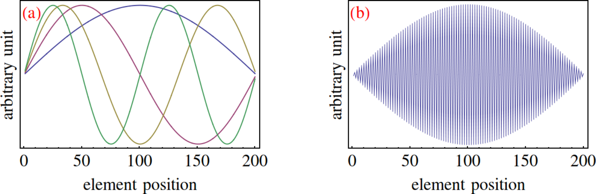
In Figure 1, a few eigenvectors are plotted as a function of their element number . In Figure 1(a), , and are plotted and are all oscillatory functions of , where the th eigenvector is identified by oscillation nodes. is also plotted in Figure 1(b). The relevant observation here is that all of these eigenvectors are extended over the entire element-position domain.
We now would like to show that randomness can localize the eigenvectors of over the element-position domain. For this part, lets preserve the tridiagonal character of as presented in Eq. 1, but add a small random number to each off-diagonal element. The new, slightly randomized is formally defined as
| (2) |
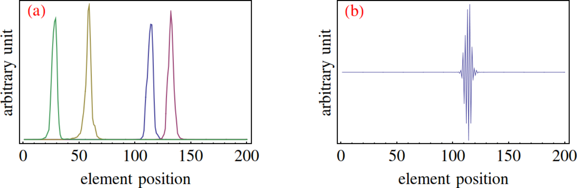
where is a number randomly selected from a real uniform distribution in the range . Similar to the case of the ordered in Figure 1, , and are plotted in Figure 2(a) and is plotted in Figure 2(b). This time, all of these eigenvectors appear to be localized over the element-position domain.

Not only does the randomness result in localized eigenvectors, but also the relative strength of randomness compared with the average off-diagonal values determines the size of the localization (localization length). This can be verified by increasing the range of the random numbers to . The new, strongly randomized is formally defined as
| (3) |
Again, the same eigenvectors are plotted in Figures 3(a) and 3(b). The eigenvectors are strongly localized over the element-position domain because of the strong randomness in the off-diagonal elements of .
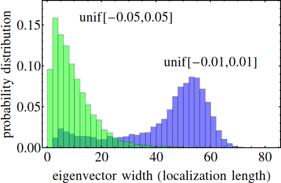
The impact of disorder on the distribution of the width of the eigenvectors on the element-position domain can be easily visualized in a histogram. In Figure 4, the distribution of the width of the eigenvectors is plotted for the weak disorder of Eq. 2 and the strong disorder of Eq. 3. The width is calculated using the second moment method, which is the standard deviation around the mean position calculated using the absolute-value-squared of the eigenvectors. The width for the eigenvector is given by
| (4) |
Each probability distribution is presented in a histogram and is the result of averaging over 100 independent random simulations. From the distributions in Figure 4, it is clear that stronger disorder results in stronger localization of the eigenvectors; moreover, it is clear that such statements can only be made in a statistical sense. Therefore, in the case of strong disorder, although the majority of the eigenvectors are more localized, a minority of the eigenvectors may actually be less localized than those of the weak disorder.
The exercise presented here shows how off-diagonal disorder results in localization. Similar localization behavior can be observed for diagonal disorder, where only the diagonal elements of are randomized, and also for mixed diagonal and off-diagonal disorder.
Highlights:
- •
The eigenvectors of random matrices can be localized in the element position space.
- •
Some modes are very narrow and some are wide, and localization is only meaningful in a statistical sense.
- •
By calculating the width of the eigenvectors of a large ensemble of random matrices, it is possible to calculate the probability distribution for the width of the eigenvectors.
- •
A stronger level of randomness shifts the eigenvector-width probability distribution to smaller width values, hence a stronger localization.
3 Normal transmission through a random stack of dielectrics
Another interesting example that links randomness to localization is the problem of light transmission through a random stack of dielectrics. The normalized transmission through a stack of dielectrics is shown in Figure 5. The light, which is incident from the left, is partially reflected from the stack, while the rest is transmitted through the stack. The dielectrics are assumed to be lossless.

Figure 5(a) shows a periodic array of two different dielectric materials identified with refractive indexes and , more commonly referred to as a Bragg grating. Figure 5(b) is similar, except the thickness of the layers is chosen randomly.
In Figure 6(a), the relative optical power transmission is plotted as a function of the normalized frequency. The thickness of each layer is (identical for all layers), and is the wavevector, where is the optical wavelength in vacuum. The stack is made of 200 air-glass layers (400 layers total), where and is assumed. The usual bandgaps and bandpasses are observed in the transmission plot of this periodic Bragg grating.
The setup for Figure 6(b) is identical to that of Figure 6(a), except the thickness of each layer is chosen from a uniform random distribution in the range . Unlike the periodic Bragg grating, transmission through the random stack is nearly zero except for very small values of the normalized frequency . Therefore, the random stack behaves like a nearly perfect mirror beyond a certain frequency.

The calculation of the optical transmission in Figure 6 is carried out using the transmission matrix defined in Eq. 5 related to Figure 7:
| (5) |

In Figure 6, the matrix can be used to relate the right- and left-moving components of the optical field in dielectric to those in dielectric according to
| (6) |
The total transmission and reflection can be calculated by cascading all the matrices for different random layers of the dielectric stack, as discussed in detail in Ref. [39].

It is instructive to repeat the exercise of Figure 6 with a larger number of layers. In Figure 8, the number of layers is increased to 10,000 in each case, and the relative optical power transmission is plotted in dB units. The logarithmic scaling on the vertical axis shows that the bandgap frequency ranges in the ordered stack of Figure 8(a), although not perfect due to the finite number of layers, attenuate the transmitted light by more than 20,000 dB, making the stack a nearly perfect mirror over this frequency range. The random stack in Figure 8(b), except for low frequency values, is also a very good reflector. Although the attenuation in transmission at 3,000 dB or more is not as good as the bandgap region in the periodic case, it is very broadband and is not limited to bandgap range.
The observations in Figure 8 bring about a somewhat philosophical issue. In practice, any stack of optical dielectrics has some inevitable randomness; therefore, given a sufficiently large number of layers, it acts as a perfect mirror beyond a certain frequency. Of course, at very low frequencies, the wavelength is so large that it hops over the stack and results in large transmission. Therefore, in practice, any stack of optical dielectrics with a sufficiently large number of layers is a practically a broadband bandgap structure. The periodic structure analyzed in Figure 8(a) can be viewed as the limiting case of the random structure, when the randomness goes to zero. When this limit is taken, the bandpasses emerge out of the broadband bandgap of the more general disordered stack. Therefore, the philosophical point of view is that the magic of a periodic structure is not in its bandgap, because the bandgap comes naturally in any practical 1D stack; rather, it is the emergence of the bandpasses that makes periodic structure so special. While this may seem like an inconsequential philosophical issue, it is necessary to alert students who learn about coherent waves in periodic systems in optics or condensed matter physics to ensure that they develop proper early intuition about the true implications of periodicity. The bandpasses are at least as glorious as the bandgaps.
The low-frequency behavior, as well as the periodic “very weak” resurrection of transmission in Figure 8(b), can be intuitively understood based on the work of Berry et al. [40]. They have shown that the optical transmission through a random stack of bi-layered transparent plates, each contributing a random phase belonging to a uniform distribution , is given by
| (7) |
Using , , and , one obtains , which is in agreement with the numerical simulation in Figure 8(b). In the simulations presented in Figures 6 and 8, it was assumed that ; therefore,
| (8) |
In order to obtain the near uniform distribution of , the upper bound in Eq. 8 can be set to , where one obtains
| (9) |
as the condition for the disorder-induced localization, exerting its full power and agreeing with the assumptions of Ref. [40]. It should be noted that this value is very close to the value of in Figure 8(b), beyond which the attenuation is strong. Therefore, the main reason that the attenuation is not strong at low is that the random phase does not cover the entire range of . For , although the range of the phase covers the entire , it partially folds over and makes the distribution of non-uniform over .
For example, consider the case of . is a phase variable for which ; therefore, covers the entire range but with twice the probability in the range compared with range and is no longer uniformly distributed over . This is the main reason behind the partial resurrections of transmission observed in Figure 8(b) for .
A final and important point is that the exponential decay of the optical amplitude in the disordered stack is a manifestation of the “coherent” superposition of partial waves that reflect and transmit at each boundary. The fact that the naive ray theory, which is based on incoherent transmissions and reflections, fails to predict the Anderson localization behavior observed in these examples= defies the intuition at first glance. The interested reader can consult Ref. [40] for a more detailed discussion on these points. A simple and elegant experiment using a laser pointer and a stack of overhead transparencies is also presented in Ref. [40], which can be excellent demonstration in an undergraduate laboratory in optics.
Highlights:
- •
Optical transmission through a stack of dielectric layers with differing refractive indexes and random thicknesses drops, on the average, exponentially with the number of layers.
- •
This exponential drop is observed for all wavelengths that are comparable or shorter than the mean thickness of the dielectric layers. The random stack behaves like an ultra-broadband mirror.
- •
The optimum localization is obtained when the cumulative optical phase in each layer is from a uniformly distributed random number in the range . If the domain is smaller, or even larger such as , the localization is weaker.
4 Oblique transmission through a random stack of dielectrics
The example presented in section 3 can be readily generalized to the case of light incident at an angle on the dielectric stack, as illustrated in Figure 9.

The calculation can be carried out using a simple generalization of the transmission matrix defined in Eq. 5 to the case of incidence at an angle (see for example Ref. [39]).

In Figure 10, the relative optical power transmission is plotted as a function of the normalized frequency for oblique incidence at a 45∘ angle (as measured in the air layer) for the TE (transverse electric) polarization of light. Figure 10 should be compared with Figure 8, which was for the case of normal incidence.
In the case of the periodic dielectric stack in Figure 10(a), the bandgaps are shifted compared with normal incidence in Figure 8(a) and are wider and deeper. For the random dielectric stack in Figure 10(b), the transmission is lower over the entire frequency band compared with Figure 8(b); however, besides the lower value and frequency shifts of the features in transmission, no substantial qualitative difference exists between oblique incidence at a 45∘ angle and normal incidence.

The case of a TM (transverse magnetic) polarization is explored in Figure 11, where the periodic-stack bandgaps in Figure 11(a) are substantially narrower and more shallow compared with the case of a TE polarization at 45∘ angle in Figure 10(a) and normal incidence in Figure 8(a). Similarly, the transmission of the TM polarization at 45∘ angle in Figure 11(b) through a random stack is stronger in the case of a TM polarization compared with the TE polarization in Figure 10(b) and the case of normal incidence in Figure 8(b).

For the larger incidence angle of 85∘, the difference between transmission through a periodic dielectric stack and a random dielectric stack is more pronounced; and so is the difference between TE and TM poalizations. The bandgaps are wider and deeper (note the dB label in the vertical scale) for the TE polarization incident on a periodic dielectric stack in Figure 12(a) compared with the case of 45∘ and the case of normal incidence. The gaps are also shifted in normalized frequency and are more widely separated. Similar behavior is observed for the case of the TE polarization incident on a random dielectric stack in Figure 12(b), where the full strength of the localization begins at a higher normalized frequency than what is shown in Figure 12(b); this behavior agrees with the general shift of the spectral features to the higher normalized frequency observed in the case of a periodic dielectric stack in Figure 12(a).

For the TM polarization incident on a periodic dielectric stack in Figure 13(a), many narrow and closely separated gaps appear in the studied normalized frequency range. The gaps are deeper compared with the case of 45∘ and the case of normal incidence. Similarly, the spectral features shift to lower values in the case of the TM polarization incident on a random dielectric stack in Figure 13(b); therefore, the full strength of the localization begins at a lower normalized frequency compared with TE polarization and smaller incidence angles (for both polarizations).
TM polarization and Brewster’s angle
In the above examples, it is observed that the TM polarization behaves differently from the TE polarization. The root of this distinction is in the different boundary conditions for the electric field in the TE and TM polarizations at the interface of each layer, and the difference is most apparent at Brewster’s angle, while the TM polarization shows perfect transmission. In Figure 14, the relative optical power transmission is plotted as a function of the incidence angle of the TM polarized light on a random dielectric stack for (a) , and (b) . Perfect transmission is observed at Brewster’s angle through 10,000 glass-air layers of random thickness. Of course, like other simulations so far, intrinsic attenuation of glass is neglected in these simulations. The transmission is lower (localization is stronger) for in Figure 14(b) compared with the case of in Figure 14(a), as expected from previous simulations and related arguments.


For comparison, in Figure 15, the relative optical power transmission is plotted as a function of the incidence angle of TE polarized light on a random dielectric stack for (a) , and (b) . Compared with Figure 14, the absence of perfect transmission at Brewster’s angle is notable. It can also be concluded that below Brewster’s angle, transmission is weaker in the TM polarization compared with the TE. This is expected, because at normal incidence TE and TM polarizations have the same transmission; increasing the angle results in a monotonic increase in transmission for the TM polarization all the way up to 100% at Brewster’s angle, while the transmission for the TE polarization monotonically decreases. Beyond Brewster’s angle, the TE polarization continues its slow decline; however, the TM polarization goes through a steep decline. Depending on the value of , at large angles, the TM polarization will have a lower transmission compared with TE (compare Figure 14(a) with Figure 15(a)), or vice versa (compare Figure 14(b) with Figure 15(b)). The interested reader is encouraged to consult a detailed account of the polarization dependence of an obliquely incident light on layered media in Ref. [41].
Random dielectric stack as a broadband waveguide
Based on the detailed discussions of the oblique incidence e.g., the results in Figure 14 and Figure 15, it is conceivable to make a 1D waveguide in the form shown in Figure 16. For a periodic dielectric stack, a waveguide can efficiently operate over a narrow range of wavelengths in the bandgaps corresponding to the specific incident wavelength [42, 43, 44]. The operating bandwidth can be increased by considering a chirped grating as shown in Ref. [45]. Alternatively, a design based on a random dielectric stack is very broadband; the trade off is that the leakage is slightly higher than that of a bandgap design for a periodic dielectric stack. Therefore, if ultra-broadband operation is desired, a random stack is likely the solution.

Highlights:
- •
Considerable differences are observed between the transmission of the TE and TM polarizations, when a random dielectric stack is illuminated at an angle. This hints at the possibility that the vectorial nature of the electromagnetic field may play an important role in setting the localization behavior in certain situations.
- •
The strongest difference between the TE and TM polarizations can be observed for oblique incidence at Brewster’s angle, at which the TM polarization is entirely transmitted through the random dielectric stack.
- •
Below Brewster’s angle, the TE polarization usually has a lower transmission; however, above Brewster’s angle, the situation depends on the ratio of the size of the optical wavelength to the average lattice size.
- •
The concept of a broadband waveguide is introduced, where the random dielectric stacks are used as broadband reflecting walls for the waveguide.
5 Transverse Anderson localization of light in one transverse dimension
Consider the one dimensional array of identical single-mode optical fibers sketched in Figure 17. The propagation constant of each fiber is and the direction of the propagation of the optical wave is assumed to be into the page. Each fiber is weakly coupled to its nearest neighbor, and the strength of the coupling is determined by the separation between the fibers. The coupled mode equations for the propagation of the optical field through this optical fiber array can be expressed as [39]
| (10) |
is the amplitude of the optical field in the th fiber, () is the coupling strength of the th fiber to its right neighbor (left neighbor ), and we assume symmetric coupling, so . Of course, we need to assume and , because the 1st (th) fiber does not have a neighbor to its left (right).

Here, we consider the simple case, where the input light is only coupled to the middle fiber at . As the optical field propagates through the middle fiber, it couples to its neighboring fibers; those will couple to their neighbors as well, and this cascading event results in a discrete diffraction pattern. This scenario is shown in Figure 18(a), where the intensity of the propagating light is plotted as a function of the propagation distance and the waveguide number. The parameters used in this simulation are: , , , and . The input boundary condition is set to , as mentioned above.

The situation is quite different if the coupling between the waveguides is randomized. For example, consider perturbing the array slightly, so that the average coupling remains , but individual couplings vary with a uniform distribution according to , where . In Figure 18(b), we observe that the light in the middle waveguide cannot spread as efficiently to its neighbors and the diffraction slows down as the beam propagates farther in . This behavior is certainly induced by the disorder and randomness introduced in the cross coupling of fibers. Therefore, it is reasonable to expect that more randomness should result in slower diffraction. This is verified in Figure 18(c) by repeating the experiment for .
Let’s take a closer look at the optical field pattern in Figure 18(c). The propagating light initially follows a diffracting pattern, but after a certain propagation distance the diffraction halts and the total width of the beam remains more or less the same for the rest of the propagation. It appears that the fibers near the edges of the array always remain dark. This behavior is referred to as transverse Anderson localization. In fact, similar behavior can be observed in Figure 18(b) after a sufficiently long propagation distance; however, the transition to a stable width occurs at a longer propagation distance and the beam width is larger because of the smaller amount of disorder.
The light propagation in a one-dimensional disordered coupled fiber array is transversely localized for any amount of disorder; however, if the disorder is too small, the stable localized beam width may be larger than the transverse size of the structure and the localization effect cannot be observed in practice.
The coupled fiber array of Figure 17 described by Eq. 10 can be analyzed alternatively in the language of normal modes. The advantage of the normal mode description is that the equations describing light propagation in a disordered coupled fiber array can be directly mapped to a random matrix discussed in section 2: the transverse Anderson localization is nothing but the localization of the eigenvectors in the element-position domain index of . In order to see this, we define the vector as
| (11) |
and rewrite Eq. 10
| (12) |
where all diagonal elements of the symmetric tridiagonal matrix are equal to and the off-diagonal elements are . The boundary condition is set to , because the input light is only coupled to the middle fiber.
The real tridiagonal matrix is symmetric; therefore, all of its eigenvectors are real and mutually orthogonal and its eigenvalues are real. We identify the th eigenvalue as and the corresponding eigenvector as , and represents the th element of the eigenvector. Furthermore, without loss of generality, we assume that the eigenvectors are properly scaled such that they are orthonormal, i.e., .
Using the eigenvectors, we can construct a real orthogonal matrix such that , where , and carry out an orthogonal transformation to rewrite Eq. 12 as
| (13) |
The orthogonal transformation of the matrix results in a diagonal matrix whose elements are the eigenvalues of , i.e., .
Using the above information, we can rewrite Eq. 13 as
| (14) |
where we have defined
| (15) |
The solutions to the independent first-order differential equations 14 for the unidirectional propagation of light can be simply written as
| (16) |
Using the orthogonal transformation and a few lines of simple algebra, Eq. 16 can be expressed as
| (17a) | ||||
| (17b) | ||||
| (17c) | ||||
Equation 17c brings the problem to its final form, using which we can now discuss the transverse Anderson localization in terms of the random matrix in the language of Section 2. Recall that we showed in Figure 2 and the corresponding discussions that the eigenvectors of a symmetric tridiagonal matrix with random off-diagonal elements are localized over the element-position domain. Therefore, only a few elements of each in Eq. 17c are non-zero. We also observed in Figure 2 that the localization of the eigenvectors occurs at different locations in the element-position domain; therefore, only very few eigenvectors have non-zero elements in the position. As a result, the sum in Eq. 17c is practically limited to only a few eigenvectors (modes) that have non-zero elements and the other non-zero elements of these few eigenvectors are all concentrated around due to localization. Therefore, will be equal to zero for all if is very different from .
From the above discussions we can conclude that for a stronger disorder, the localization becomes stronger as seen in Figure 2, and will remain zero unless is even closer to . The picture portrayed here is consistent with Figure 18, especially in describing the difference between Figure 18(b) and Figure 18(c).
Lets recap these observations in the more common modal language. The initial beam only couples to those guided modes that are localized in the vicinity of the center fiber. Near the entrance, the optical excitation closely resembles the in-coupling beam, as a result of a coherent sum of the excited modes. Each excited mode propagates with a different phase velocity determined by the propagation constant ; therefore the detailed balance between the excitation amplitudes of the guided modes that is responsible for the narrow excitation at the entrance is broken as the relative phases between the modes change when the beam propagates along the fiber array. As the beam propagates and the detailed balance is further broken, the beam expands; however, it can never expand beyond the size of its constituent modes, which are only a few, each being very localized. Therefore, the expansion is eventually halted, as observed in Figure 18(b) and Figure 18(c).
Using the modal language we can explain a few other interesting phenomena. One question that is often asked is what happens if the initial excitation is wider than the typical width of an individual mode? The answer is that a wider beam excites a few more modes; therefore, the propagating light eventually localizes to a slightly wider beam. Another interesting fact is that because in Eq. 17c only a few terms in the sum play a role, after a sufficiently long propagation distance , the beam refocuses back to its initial intensity distribution (self-imaging) [46, 47]. This revival distance can be calculated by noting that at , must be satisfied for all the relevant terms in the sum, where each is an integer. The intensity pattern at will be identical to that at . In practice, if the number of excited modes is sufficiently large, the revival distance can be much longer than the waveguide and the refocusing is not observed.
It must be noted that a similar localization behavior is obtained if instead of randomizing the coupling coefficients between the fibers in the array [48], the propagation constants of individual fibers are slightly randomized [49]. This was briefly discussed in Section 2 as diagonal localization.
Mode shapes
In Figure 19 we show the distribution of the propagation constants of the eigenmodes of the coupled waveguide array of Figure 17; i.e., in Eq. 16, for . The parameters used for the disorder relate to the case discussed in Figure 18(b), where we used , , , and , with . The calculated modes are numbered from to , sorted in a descending order of the value of the propagation constant. As expected, the calculated propagation constants are in the vicinity of . The range of variation of is determined by the range of (), while the exact values vary for each different random waveguide.

In Figure 20 we plot the shape of a few modes of the waveguide. Of course, the coupled waveguide array supports a total of modes. In Figure 20 each mode is normalized to unity for easier comparison. The horizontal axis is the waveguide number in Figure 17. Figures 20(a), (b), (c), (d), (e), (f) correspond to mode numbers 1, 25, 99, 101, 170, 201, respectively. Recall that the mode numbers here correspond to the mode numbers used in Figure 19. Therefore, Figure 20(a) is the mode with the largest propagation constant in Figure 19, which is the top edge of the propagation constant band.

The modes that correspond to the region in the vicinity of the top edge of the band are highly localized with very few oscillations. As the propagation constant is increased e.g., for mode number 25 the mode profile oscillates a few times as in Figure 20(b). The modes near the middle of the band in the vicinity of generally oscillate rapidly and spread over many waveguides, as can be seen for modes number 99 and 101 in Figures 20(c) and (d), respectively. These modes become more localized if the disorder is increased. Once the mode number gets closer to the bottom edge of the band, the oscillations become so rapid that the sign of the mode profile flips between adjacent waveguides, and the modes localize again. This behavior can be clearly seen for modes number 170 and 201 in Figures 20(e) and (f), respectively.
The mode width is plotted against the propagation constant of each mode in Figure 21, averaged over 1000 simulations for (a) and (b) . It is clear that the band edges result in the narrowest modes, while the modes near the middle of the band are more spread out. Also, the stronger disorder in Figure 21(b) results in smaller mode widths compared with the weaker disorder case in Figure 21(a).

The disorder in the model studied here is off-diagonal. Although the effects of diagonal and off-diagonal disorder are generally quite similar, there exist subtle differences between the two types of disorder. For example, it has been argued that while all modes are exponentially localized for diagonal disorder, this may not be strictly true for off-diagonal disorder [50, 51, 52]. Specifically, the modes at the center of the band in a 1D off-diagonally disordered lattice fall off asymptotically as instead of the simple exponential form , where represents the distance from the center of the mode at . The form is also responsible for the divergence of the mode width in the middle of the band in both subfigures of Fig. 21. We emphasize that even in the middle of band, the mode is localized, although the weaker localization form results in a divergent mode width. There are also differences between diagonal and off-diagonal disorder in 2D that will be pointed out later in section 6.
Beam width in position and momentum space


In Figures 25, 25, 25, 25, we explore in some detail the expansion and localization of the optical beam that is coupled to the waveguide array of Figure 17, as a function of the longitudinal coordinate. The vertical axis is the beam width, which is determined by the second moment method of Eq. 21. The parameters used for the disorder relate to the cases already discussed in Figure 18. For these figures we have used , , and . Any figure labeled with (a) corresponds to the disorder-free periodic array; labeled with (b) corresponds to the weakly disordered case of , where ; and labeled with (c) corresponds to the strongly disordered case of . The only minor differences are that , and the boundary condition is set to
| (18) |
We note that the beam width formula of Eq. 21 (presented later in this article) also gives the value of for the beam width at .
Figure 25(a) shows the expansion of the beam width in the disorder-free lattice. The expansion is ballistic, i.e., the width grows linearly with propagation distance (at large ). In Figure 25(b) we plot the expansion of the beam width for three sample realizations of the random waveguide for the weakly disordered case, as explained above. The tendency to localize can be seen in each of these samples, but one can immediately see the random nature of the process, where different random realizations of the coupled waveguide system result in different rates of initial expansion and final beam localization width. Lastly, the expansion of the beam width for three sample realizations of the random waveguide for the strongly disordered case is shown in Figure 25(c). Note the different vertical scale in these three subfigures. It is clear that despite the random variation the disorder slows and eventually halts the expansion, and a stronger disorder results in a smaller eventual localization width on average.
It is interesting to study the beam expansion in the Fourier -space (momentum space) as well. A well-known characteristic of the ballistic expansion of the beam is that the beam width in the -space remains invariant under propagation, as shown in Figure 25(a). The -space expansion of the cases plotted in Figures 25(b), (c) are shown in Figures 25(b), (c). Interestingly, the beam widths in the -space conform well to our intuition that narrower beams in -space are wider in -space; of course, this simplistic intuition is not always true, especially in the presence of spatial chirp.
As was noted above, the statistical nature of Anderson localization means that the beam expansion rate and the eventual localization width varies depending on the particular “random” realization of the disordered waveguide. Therefore, no two propagations will be identical. However, some general conclusions can still be drawn, in a statistical sense, about the average beam width, as well as the variation around the average. In Figure 25 we show the average beam width over 100 independent statistical realizations of the disordered waveguide, plotted as a function of the longitudinal propagation coordinate . Figure 25(a) is the disorder-free ballistic propagation and is plotted again for comparison with Figures 25(b) and (c), which correspond to the weakly and strongly disordered cases, respectively. The vertical scales in these subfigures are all chosen identically, for easier comparison. It is clear that, on average, the localized beam width is narrower for the case of a stronger disorder, as expected. The error bars in Figures 25(b) and (c) signify one standard deviation for the beam width around the mean over the 100 independent random samples. Strong disorder results, not only in a smaller beam width, but also in a smaller variation around the average beam width. Therefore, a stronger disorder is equivalent to a better predictability: when the disorder is strong, the beam width is smaller and is almost the same in all random realizations of the disordered waveguide.
Finally, in Figure 25 we plot the corresponding average beam width in -space, where the error bars are now defined as the one standard deviations of the beam width in -space. The interested reader is urged to consult Refs. [53, 54, 55, 37] for a more detailed account of the beam expansion in 1D and 2D disordered lattices e.g., it is argued that in a 2D disordered waveguide the expansion starts as ballistic then goes through a diffusive phase, and eventually the localization takes over. However, in 1D the diffusive transport regime is absent and the expansion turns from ballistic directly to localized.
Highlights:
- •
The light propagating through a coupled array of identical optical waveguides remains confined to only a few waveguides (transversely localized), if the waveguide-to-waveguide couplings are random.
- •
Similar localization behavior can be observed if the individual waveguides are randomized, regardless of whether the waveguide-to-waveguide couplings are random or not.
- •
The stronger the disorder, the more localized the beam is.
6 Transverse Anderson localization of light in two transverse dimensions
Transverse Anderson localization in two transverse dimensions can be explored in a similar fashion to 1D transverse localization discussed in the previous section. Consider the 2D array of optical fibers placed in a hexagonal lattice in Figure 26. The hexagonal lattice is special because each fiber has six nearest neighbors separated by an equal distance , and the next-to-nearest separations are . In contrast, a fiber in a square lattice has four nearest neighbors and the next-to-nearest separations are . Therefore, the next-to-nearest couplings are weaker in a hexagonal lattice and the simplifying assumption of the nearest neighbor coupling is more reliable.

Similar to Eq. 10, the coupled mode equations for the propagation of the optical field through this optical fiber lattice can be expressed as
| (19) |
where the sum is only on the nearest neighbors, and the coupling matrix is symmetric.
As we discussed in the previous section, the transverse Anderson localization can be explored by studying the distributions of the elements of eigenvectors of the matrix over the element position space. Here, is the effective propagation constant matrix of the coupled fiber system and is defined as , noting that are non-zero only when and are the nearest neighbor fibers. The fiber coupling constants are assumed to be random in the general form of , where is a fixed value of and belongs to a random distribution. Here, we take and on a hexagonal lattice of fibers.
In Figure 29 we consider the non-random deterministic case with . The magnitude of the four eigenvectors of the matrix with the largest eigenvalues are shown as density plots on the element-position domain of the hexagonal lattice. For the reader familiar with coupled mode theory, the calculated eigenvectors are the supermodes of the entire waveguide structure [56]. The left most figure shows an azimuthally symmetric distribution of non-zero elements that decrease monotonically from the center of the lattice toward the boundary. Other eigenvectors have different distributions and symmetry properties, but they all nearly fill the entire element-position domain, i.e., the non-zero elements of the eigenvectors spread over nearly the entire lattice.

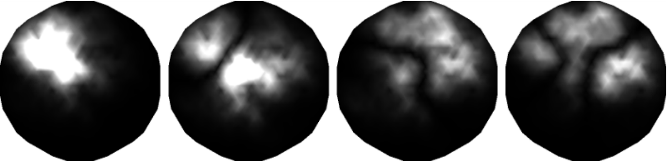
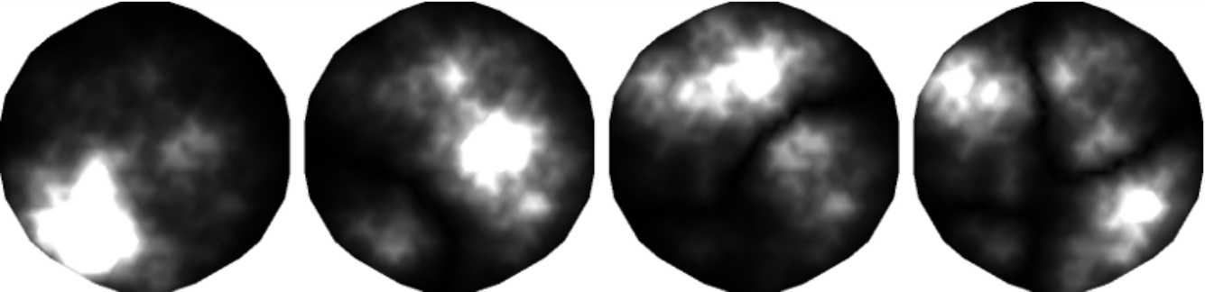
Let’s consider what happens when the coupling constants are randomized according to in Figure 29. Similar to the above, the magnitude of four eigenvectors of the matrix are shown as density plots on the element-position domain of the hexagonal lattice. All figures show that the non-zero elements of the eigenvectors are localized in certain regions on the lattice, as expected from the transverse Anderson localization. Of course, the localization region for each eigenvector is different.
As mentioned before, random variations of the diagonal elements of the matrix can also induce localization of the eigenvectors in the element-position domain. This is shown in Figure 29, where the off-diagonal elements are assumed to be constant values of and the diagonal elements (propagation constants of the individual optical fibers) are randomized according to , where . Therefore, the effect of the diagonal disorder is similar to that of the off-diagonal disorders, at least qualitatively. Of course, transverse Anderson localization is similarly observed if both diagonal and off-diagonal disorder are implemented simultaneously. Transverse Anderson localization in a 2D lattice of optical fibers with random variations of the parameters was first proposed by S. S. Abdullaev and F. Kh. Abdullaev of the Heat Physics Department of Uzbekistan Academy of Sciences in 1980 [29].
Earlier in this tutorial review, we briefly highlighted the subtle differences between diagonal and off-diagonal disorders in a 1D disordered lattice. The weaker localization in the middle of the band for off-diagonally disordered lattices persists in 2D as well. For example, it has been argued in Ref. [57] that in the middle of the band for a 2D disordered square lattice, the wave amplitude falls off with distance as where is the distance from the center of the mode and is an exponent that depends on the amount of disorder. The power-law localization is also attributed to the geometry of the square lattice (and the logarithmic singularity of the density of states in the middle of the band). Therefore, for the triangular lattice that has been studied in this section (which does not have a logarithmic singularity of the density of states in the middle of the band), all modes are exponentially localized.
Highlights:
- •
Transverse Anderson localization is observed for a 2D disordered coupled waveguide array, just as in 1D.
7 Transverse Anderson localization of light: the RLV mechanism
The 2D transverse Anderson localization of light that was proposed by Abdullaev and Abdullaev and discussed in the previous section strongly resembles the original proposal by P. W. Anderson. We will refer to this as the AA mechanism for the rest of this article, not to be confused with the Aubry-Andre model [58]. In either case, the starting point is a lattice-periodic potential where each site on the lattice is characterized by a “bound-state” energy ( for fibers) and off-diagonal couplings ( for fibers). In the absence of randomness, the solutions to the wave equations are Bloch-periodic solutions that extend over the entire lattice. If sufficient randomness is introduced in the energy and/or couplings, the solutions of the wave equation no longer extend over the entire lattice; rather, they localize to certain regions on the lattice.
An alternative method to obtain the 2D transverse Anderson localization of light was independently proposed by de Raedt, Lagendijk, and de Vries in 1989 [30]. Recall that for the AA mechanism, the disorder was introduced on top of an existing ordered lattice. However, in the suggested method by de Raedt, Lagendijk, and de Vries (RLV mechanism), the randomness is not superimposed on top of an existing ordered lattice; rather, the underlying potential is completely random [30]. De Raedt et al. [30] proposed that this scheme can be realized in a quasi-2D optical system in a dielectric with a transversely random and longitudinally uniform refractive index profile. This is sketched in Figure 30a, where a long dielectric “waveguide” has a random refractive index profile that is invariant along the fiber. De Raedt et al. suggested a binary random system, where each pixel is randomly chosen to have a refractive index of or with equal probabilities, where and are marked by red and blue color, respectively in Figure 30a.
Using extensive numerical simulations, De Raedt et al. showed that for a properly designed random fiber e.g. with , ; and , where is the width of each pixel and is the wavelength of light, they obtain quasi-2D localization in the transverse plane of the waveguide. An optical field that is launched in the longitudinal direction initially expands until it reaches a terminal localization radius, after which the freely propagating beam fluctuates around a relatively stable radius. In Figure 30b, a slice of the intensity distribution in the - plane is shown for a representative localized propagation through a random binary waveguide, where is a transverse coordinate and is the longitudinal coordinate.

Highlights:
- •
One way to observe transverse Anderson localization is to use a 2D disordered coupled waveguide array. We refer to this as the AA mechanism because it was originally proposed by Abdullaev and Abdullaev.
- •
Alternatively, transverse Anderson localization can be observed in a optical fiber-like medium with a fully random refractive index profile. We refer to this as the RLV mechanism because it was originally proposed by de Raedt, Lagendijk, and de Vries. The RLV mechanism is distinct from the AA mechanism by the absence the underlying lattice.
8 Experimental observation of localization: the AA mechanism
The first experimental observation of the transverse Anderson localization of light was carried out in Segev’s group in 2007 [59]. The experiment was more in line with the AA mechanism discussed earlier in section 6, where the disorder was superimposed on top of an existing triangular lattice of waveguides. The ordered lattice and the superimposed disorder were formed, by means of the optical induction technique [60], in a photo-refractive crystal (SBN:60) using a laser beam at 514 nm wavelength.
In order to write the underlying ordered lattice in the photo-refractive crystal, Schwartz et al. [59] used the interference pattern generated by three symmetrically arranged lasers and obtained a fully periodic hexagonal interference pattern with periodicity of 11.2 µm inside the 10 mm-long crystal. The disorder is generated from a speckled beam that is invariant in the longitudinal direction, as required for the observation of transverse Anderson localization. The speckled beam was formed from a Bessel beam, created by passing a Gaussian laser beam through an axicon, and then passed through a 4-f imaging system, where a diffuser was placed at the joint Fourier plane between the two lenses. The 4-f imaging system with the diffuser transformed the Bessel beam into a broad and speckled beam that was coherently combined with the original lattice-forming beam to create the desired refractive index fluctuations on top of the ordered lattice in the photo-refractive crystal.
In order to investigate the localization, Schwartz et al. used another probe beam at 514 nm wavelength. The beam width was 10.5 µm full-width at half-maximum (FWHM) and was always launched into the crystal at the same location. In the absence of disorder, they observed diffraction patterns after 10 mm of propagation. They observed clear transverse localization of the probe beam when the disorder level was increased to more than 30%. In order to obtain an appropriate ensemble to calculate the mean localization radius (localization length), the diffuser was rotated by a step-motor, such that the laser beam passed through a different location on the diffuser in each step, where a new intensity measurement was taken.
For the large disorder level of 45%, Schwartz et al. fitted the properly averaged intensity distribution of the localized beam, over 100 independent experiment, to an exponential of the form , and obtained =64 µm for the localization length of the Anderson localized beam. The experiment carried out by Schwartz et al. was quite interesting, as they were able to vary the disorder level by controlling the intensity level of the disorder-inducing lasers, and also obtained an ensemble of independent measurements for the statistical analysis of the localization phenomenon by rotating the diffuser. However, the variations of the refractive index of random sites in Ref. [59] were on the order of . As we will discuss later in greater detail, the radius of the localized beam (localization length) depends on the magnitude of the refractive index fluctuations. In order to obtain a more localized beam for device applications e.g., comparable to the beam radius in a conventional optical fiber, it is necessary to increase the magnitude of the index fluctuations [61]. Moreover, when the magnitude of the index fluctuation is larger, the sample-to-sample variation in the beam radius becomes smaller; therefore, each element of the ensemble closely resembles the average. This self-averaging behavior alleviates the need for averaging over a large ensemble, and for a sufficiently large magnitude of the index fluctuation the average is almost identical to each element. We will discuss a recent realization of the transverse Anderson localization in the presence of a large index contrast in the next section.
Highlights:
- •
The first observation of transverse Anderson localization was reported by Schwartz et al in an AA-mechanism setup.
- •
The underlying lattice and the overlaying disorder were optically induced in a photo-refractive crystal. A separate beam was used to probe the localization behavior.
- •
The setup allowed them to vary the amount of disorder on demand.
9 Experimental observation of localization: the RLV mechanism
In section 7 we discussed the RLV mechanism for the transverse Anderson localization of light. The quasi-2D system proposed by De Raedt et al. [30] strongly resembles an optical fiber. In 2012, Karbasi et al. [17] designed and fabricated an optical fiber that functioned based on the RLV mechanism, i.e., transverse Anderson localized in the presence of an entirely random refractive index profile. In order to obtain the random and pixelated refractive index profile of the RLV mechanism, Karbasi et al. [17] used 40,000 pieces of a low index polymer fiber polymethyl methacrylate (PMMA) with refractive index of 1.49 and 40,000 pieces of a high index polymer fiber polystyrene (PS) with refractive index of 1.59. Each fiber was 8 inches long with an approximate diameter of 200 µm. The fibers were randomly mixed, assembled to a square preform as shown in Figure 31, fused together, and redrawn to a fiber with a nearly square profile and approximate side width of 250 µm [62].

We recall that one of the requirements for transverse Anderson localization is the longitudinal invariance. Some of the randomly mixed optical fibers may have crossed over each other during the assembly and redraw process; however, the large draw ratio of the fiber guarantees that the refractive index profile remains relatively unchanged along the fiber. Moreover, small perturbations are likely not going to disturb the transverse localization noticeably.
Figure 32 shows the scanning electron microscope (SEM) image of a polished polymer Anderson localized optical fiber (pALOF). Figure 32a is the image of the cross section of the optical fiber with an approximate side width of 250 µm, where the high and low index regions are not distinguishable in this figure. Figure 32b is a zoomed-in SEM image of a 24 µm wide region on the tip of pALOF exposed to 70% ethanol solvent to to dissolve the PMMA, so that the PMMA region can be differentiated by the darker color. The sizes of the random features (pixels) in Figure 32b are around 0.9 µm.

In order to investigate the guidance and localization properties of the pALOF, light from a single mode optical fiber was directly launched (nearly butt-coupled) into the pALOF. The output near-field image was collected by a 40X objective and was projected onto a CCD camera. Figure 32c shows an experimental measurement of the near-field intensity profile of the localized beam after 60 cm of propagation through pALOF, where the wavelength of light is 633 nm. The localization was observed to be strong: when the input beam was scanned across the input facet, the output beam clearly followed the transverse position of the incoming beam [63].
We encourage the interested reader to consult Ref. [64] for another method to obtain transverse Anderson localization based on the RLV mechanism. The optically induced randomized potential is created by a computer controlled spatial light modulator (SLM) in a photorefractive crystal.
Highlights:
- •
Experimental observation of transverse Anderson localization for the RLV mechanism was reported by Karbasi et al in a disordered optical fiber medium.
- •
The disordered fiber was drawn from a random preform. The preform consisted of 80,000 strands of optical fibers with different refractive indexes that were randomly mixed and fused together.
- •
When the input beam was scanned across the input facet, the output beam clearly followed the transverse position of the incoming beam
10 Detailed analysis of the RLV localization scheme
An attractive feature of the pALOF is the large index contrast of 0.1 that is helpful in reducing the localization radius (localization length) of the beam. The measured value for the localization radius was reported as 31 µat 633 nm wavelength. The measured radius was only slightly larger than the calculated value; however, the measured standard deviation of 14 µm was considerably larger than the variations calculated numerically and reported in Figure 3 of Ref. [17]. The measured standard deviation for the beam radius was taken from 100 separate measurements of the beam profile radius with 20 different fiber samples and 5 different locations across the fiber. This discrepancy between the theoretical and experimental variation of the beam radius was mainly attributed to the quality of the polishing of the pALOF tip as the surface quality of a polished polymer optical fiber tip is generally lower than what is routinely achievable for glass optical fibers.
Numerical modeling of wave propagation in a disordered fiber
The simulation of light propagation in a disordered fiber is carried out by numerically solving the wave propagation equation Eq. 20 using the finite difference beam propagation method (FD-BPM) [63, 59, 65].
| (20) |
Eq. 20 is the paraxial approximation to the Helmholtz equation, where is the slowly-varying envelope of the primarily transverse electric field centered around frequency and . is the (random) refractive index of the optical fiber, which is a function of the transverse coordinates, and is average refractive index of the fiber. The forward propagation scheme is implemented using the fourth order Runge-Kutta method [66].
The stability condition for the fourth order Runge-Kutta method limits the size of the steps in the longitudinal direction as , where is assumed to be the size of the transverse grid in the finite-difference numerical scheme, and in a uniform medium. In the simulations in Ref. [63], is chosen in Ref. [63] to ensure stability and no power dissipation for reliable long distance propagation. While transparent boundary condition [67] is implemented, the size of the simulation domain is taken to be large enough to ensure that the total power in the simulation region remains unchanged along the fiber for Anderson localized beams.
A typical reliable simulation of transverse Anderson localization e.g. for pALOF, requires a transverse area in the range of . The random refractive index pixel size is on the order of a wavelength, and each pixel must be resolved by roughly 10 points in each direction in the finite difference scheme; therefore, points are required in the transverse domain with . This results in the fourth order Runge-Kutta stability criterion of the form , which is for . For 500 nm, 1 nm, and for a typical propagation distance of 1 cm required for reliable localization, steps in the longitudinal direction are required, which is computationally intensive.
The effective beam radius (localization length) is calculated by the variance method [30] as
| (21) |
where the angle brackets denote integration over transverse coordinates. is the transverse position vector and is the vector pointing to the center of the beam, defined as the mean intensity position by . The optical field is assumed to be normalized according to .
We note that an estimate of the localization length is sometimes given using a quantity called the Inverse Participation Ratio (IPR) [59]. IPR is defined as
| (22) |
where is the optical intensity defined in the transverse plane, at the longitudinal coordinate . IPR has units of inverse area and the average effective width is defined as , where represents the statistical averaging over the ensemble. We note that IPR as defined by Eq. 22 is originally rooted in the definition of the mode effective area in nonlinear optics (see e.g. [68]). Equation 21 used by De Raedt et al. [30] is likely a better representation of the localization phenomena and more true to the random-walk nature of the scattered wave. Therefore, we prefer to use the second moment method of Eq. 21, rather than the Inverse Participation Ratio to calculate the localization length.
Small localized beam radii with low variations are desired
The experimental realization of the RLV scheme by Karbasi et al. [17] showed that the transversely disordered optical fibers can be embraced as a completely new class of optical fibers that guide light, not in a conventional core-cladding setting, but by means of the Anderson localization, where any location across the transverse profile of the fiber can be used to guide light. As we will see later in image transport applications of this disordered optical fiber, a small beam localization radius is likely its main desired attribute. A reduced variance is also desired, because as a device it is not helpful to have variations in the beam radius that depend on the transverse location of the beam in a random and unpredictable way. In other words, although the underlying waveguiding mechanism is based on disorder and randomness, the main measurable device attribute, the localized beam radius, should be predictable. These considerations lead one to ask what can be done, in the design of these disordered fiber in order to minimize the localization radius and also reduce the sample-to-sample variations in the localization radius.
Design parameters upon which the beam radius depends
The localized beam radius can depend on: the input characteristics of the optical beam such as the wavelength and the in-coupling beam diameter; the dimensionful fiber characteristics such as the transverse dimensions of the fiber, the width of each pixel; and the dimensionless fiber characteristics such as the refractive index of the components, especially the index difference, and the geometrical ratio of the components used in the fiber characterized by the fill-fraction.
Given the intuition we established based on the modal picture, we learned that if the initial excitation width is smaller than the radius of a typical mode of the disordered waveguide (localization radius or localization length) , the propagating light eventually localizes to a radius that is comparable to the localization length; and if the initial excitation is wider than the typical width of an individual mode, the propagating light eventually localizes to a slightly wider beam than the original size. Therefore, the design program to optimize the disordered waveguide for best localization must be independent of the input beam profile and must focus on the transverse dimensions of the localized beams [69, 70, 71].
Another important property of the disordered fiber is the transverse size of the fiber. If the fiber cross section is not large enough, the boundaries of the fiber strongly affect the localization radius of the modes. The impact of the boundary on the localization radius of the modes that reside near the boundary is inevitable, but in an ideal case the fiber cross section must be large enough so that the modes in the interior region are shielded from the boundary to prevent excessive scattering loss; therefore, the physical characteristics of the majority or nearly all of the interior modes are solely determined by the transverse Anderson localization mechanism.
In the ideal case, when the disordered fiber cross section is much larger than the light wavelength, feature size (width of each index pixel), and the localization radius of the typical modes, the total transverse size of the fiber becomes irrelevant. In that case, the only two dimensionful fiber design parameters are the light wavelength and the width of each pixel. Considering the fact that Maxwell’s equations are scale invariant, if the wavelength and feature size (fluctuating index pixel size) are scaled by some factor, the localized beam radius of each mode is scaled by the same factor.
The feature size of the pALOF studied in Refs. [17, 63] are approximately 0.9 µm. Experimental measurements and numerical simulations have confirmed that the localization radius is much smaller at 405 nm wavelength than at 633 nm wavelength, as shown in Figure 33. It is speculated that the optimum feature size for strong localization using the RLV scheme is around . This statement is merely an educated guess and the optimum value of the feature size relative to the wavelength has yet to be found. Intuitively, if the feature size is too small compared with the wavelength, the optical field would hop over the random sites and merely average the refractive index, with very weak scattering. On the other hand, if the feature size is too large compared with the wavelength, the mean free path for wave scattering will be large, resulting in a large localization radius. Therefore, there must be an optimum value of the feature size for a given wavelength. Finding the optimum value is computationally very challenging.
Another design parameter that affects the localized beam radius in the binary disordered RLV scheme is the portion of each random refractive index component, characterized by the fill-fraction . In Ref. [63], is defined as the portion of the low-index material in the higher index host medium. Using an intuitively plausible argument that the maximum transverse scattering is obtained when there is an equal amount of low-index and high-index material in the disordered matrix, and also a few instances of simulations relevant to the experimental regime of interest, Karbasi et al. [63] have argued that should be regarded as the ideal design target. A sample simulation is shown in Figure 34, where the evolution of the effective beam radius versus the propagation distance is shown for different values of the fill-fraction of and ; and the latter provides a lower effective beam radius and localization length.
The last, but definitely not the least important design parameter to reduce the localization radius is the index difference between the random components of the disordered fiber. It is generally believed that a stronger localization (smaller average mode radius) is obtained if the refractive index difference between the random constituents is increased. This is confirmed in the 1D model of the transverse Anderson localization of Ref. [46]. However, it is also shown that the dependence of the average mode radius on the index difference asymptotically saturates beyond a certain value of the index difference; therefore, the payback in the reduction of the localization length may be quite small beyond a certain threshold index difference. While these issues are well studied in the 1D model of Ref. [46], the 2D analysis remains to be done. For the 2D geometry, Karbasi et al. [63] compared the localization radius in a glass-air disordered fiber with pALOF. The refractive index of sites in the glass-air disordered fiber are randomly picked as and for the glass host and random air-hole sites, respectively. The index difference of 0.5 in the glass-air disordered fiber compared with 0.1 in pALOF results in a considerable reduction in the localization radius. In Figure 35, the calculated beam radius versus propagation distance for different values of fill-fraction are plotted, and thelocalized beam radius is clearly smaller than that provided by the index difference of 0.1 for pALOF.
Finally, we have repeatedly observed that whenever the scattering strength is increased to reduce the localization length (localized beam radius), whether by selecting the right wavelength, or by bringing the fill-factor close to 50%, or by increasing the index difference, the statistical variation of the beam radius decreases. Therefore, we have the luxury of solving two problems with one solution (a more animal friendly expression than killing two birds with one stone!).
Spatial beam multiplexing
The possibility of spatial beam multiplexing in pALOF was studied in Ref. [18] in 2013. It was shown, both numerically and experimentally, that a pALOF can be used to simultaneously transport multiple beams [72].

In Figure 36(a) beam multiplexing in pALOF is studied numerically at 405 nm wavelength, where the intensity profile of a multiplexed beam is plotted after 5 cm of propagation along the fiber; the four exterior beams are launched at a distance of 70 µm from the central beam. The output beams do not show any appreciable drift and remain in the same transverse location across the fiber.
Experimental verification of beam multiplexing are shown in Figure 36(b), where both beams are 405 nm wavelength, and in Figure 36(c), where the upper beam is at 405 nm wavelength and the lower beam is at 633 nm wavelength. The localization is clearly stronger at 405 nm due to the choice of the design parameters of pALOF, as discussed before.
Macro-bending loss
In section 10 the possibility of beam multiplexing in an disordered fiber was discussed. Given the unconventional nature of the beam confinement in a disordered optical fiber, one must worry about the possibility that the spatially multiplexed beams drift across the fiber when the fiber is subjected to substantial macro-bending. This issue was studied in detail in Ref. [18]. Using numerical simulations, it was shown that transverse Anderson localization is very robust and can withstand, at least in theory, a degree of macro-bending that is beyond what is acceptable for conventional fibers. To explore the macro-bending experimentally, a 10 cm section of a 15 cm-long pALOF was wrapped 16 times around a mandrel with an approximate radius of 1mm, where no appreciable loss of walk-off effect was observed in the localized beam.
11 Image transport through the disordered fiber
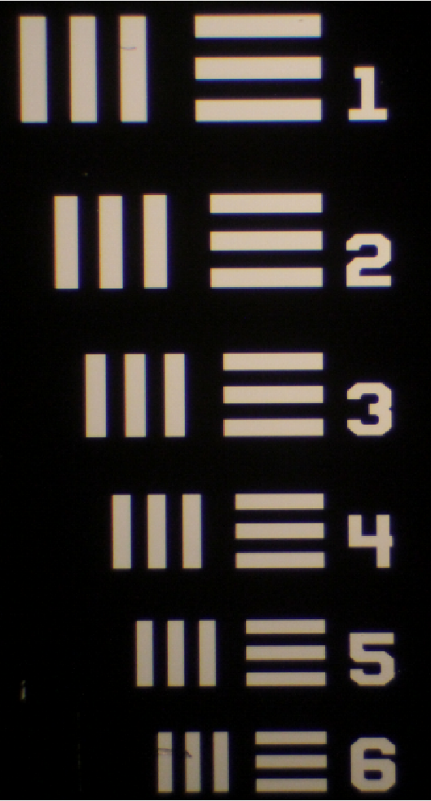


Motivated by the successful demonstration of beam multiplexing, Karbasi et al. used pALOF for endoscopic fiber-optic imaging. To their pleasant surprise, the image transport quality was comparable to or better than some of the best commercially available multicore imaging fibers, with less pixelation and higher contrast [19]. Figure 37 shows some of the transported images in the form of numbers from a section of the 1951 U.S. Air Force resolution test chart through pALOF. The test-target, in the form of a stencil in which numbers and lines were carved, was butt-coupled to the hand-polished input facet of pALOF and was illuminated by white light. The near-field output was projected onto a CCD camera with a 40 microscope objective.
The minimum resolution of the images is determined by the width of the point spread function of the disordered optical fiber imaging, which was calculated to be smaller than 10 µm at 405 nm wavelength [63]. In practice, the imaging resolution in pALOF is limited by the quality of the cleave and polishing of the fiber. The fiber surface quality is partially responsible for the distortions in the transported images in Figure 37. The high quality image transport in the proof-of-concept experiment has been achieved without any optimization in the design.
Highly multicore optical fibers, similar to those introduced in section 6, have been used for direct transportation of images in various configurations [73, 74, 75, 76]. The highly multicore fiber, often referred to as the “coherent fiber bundle,” is commonly used in medical and industrial endoscopy [73, 77, 78].
For an Anderson localized fiber, a higher amount of disorder and a larger level of fluctuation in the refractive index provides stronger beam localization, resulting in an improved image resolution. A similar statement can be said for multicore imaging fiber as well: the coherent core-to-core coupling is detrimental and blurs the image; therefore, core-to-core coupling must be suppressed by varying the size of the cores so that neighboring cores cannot couple resonantly. Also, in a multicore imaging fiber, the cores must be as close as possible to create a less pixelated image, while being very different in size so that they cannot couple efficiently even when they are close. One can view the disordered Anderson localized fiber as taking the two limits of the high-packing of the cells and the large variation of the sizes to an extreme, so that the individuality of each core is completely lost: all neighboring sites are strongly coupled, but the extreme randomness prevents light leakage and blurring.

The imaging performance of the “unoptimized” pALOF compares with some of the best commercially available multicore imaging optical fibers, as is further confirmed in Figure 38. The transported images over 5 cm of the number “6” from group 5 of the 1951-AFTT test chart are compared between pALOF in Figure 38(a), Fujikura FIGH-10-350S in Figure 38(b), and Fujikura FIGH-10-500N in Figure 38(c). The image quality of the transported image through the pALOF is clearly better than FIGH-10-350S and is comparable with FIGH-10-500N. The feature sizes in Figure 38 are on the order of 10-20 µm. The Rayleigh range for this level of resolution is approximately 0.8-3 mm, which is substantially shorter than the typical propagation length in these imaging fibers. Therefore, the imaging results are non-trivial and cannot be obtained using bulk propagation or conventional multimode fibers.
Highlights:
- •
In an Anderson localized disordered optical fiber, a smaller localized beam radius is obtained via increasing the differences between the refractive indexes of the random dielectric constituents.
- •
The feature size should be , and a fill-fraction of 50% is preferred.
- •
A stronger localization is generally accompanied by a smaller variation in the localized beam radius, resulting in a more uniform and predictable beam radius.
- •
Beam multiplexing and high-quality image transport are featured as device-level applications of the transverse Anderson localization in a disordered optical fiber.
12 Transverse Anderson localization in a disordered silica optical fiber
The first observation of Anderson localization in a silica fiber was reported in Ref. [79]. The main motivation for using a glass-air structure has been the larger index contrast that results in a smaller beam diameter (better image transport resolution), as well as a lower sample-to-sample variation in the value of the beam diameter (better image uniformity) [79]. The reported glass-air disordered fiber was drawn at Clemson University. The preform was made from “satin quartz” (Heraeus Quartz), which is a porous artisan glass. By drawing the preform, the airholes (bubbles) in the glass are stretched to form the hollow air-rods required for transverse Anderson localization. The large draw ratio sufficiently preserves the longitudinal invariance, without significant disturbance over typical lengths used in the experiments.

The cross-sectional SEM image of the disordered glass-air optical fiber is shown in Figure 39a, and a zoomed-in SEM image is shown in Figure 39b. The SEM images provide a good estimate of the refractive index profile of the fiber; the light gray background matrix is glass and the black dots represent the random airholes. The diameter of the disordered glass fiber is measured to be 250 µm. The diameters of the airholes vary between 0.2 µm and 5.5 µm. Unfortunately, the airhole fill-fraction was shown to be as low as 2% in the central regions, which was far below the ideal value of 50%, so strong localization was not observed near the center. However, Anderson localization was observed near the boundary, where the airhole fill-fraction is 8%.
More recently, transverse Anderson localization has been reported by scientists from Corning Incorporated in random airline fibers (RALF) [80]. The preform for RALF is fabricated using the outside vapor deposition (OVD) process. The consolidation process is done in the presence of 100% nitrogen gass, during which nitrogen is trapped in the blank to form glass with randomly distributed air bubbles. When the preform is drawn, the random air bubbles stretch to form random airlines. RALFs with 150, 250 and 350 µm diameters were fabricated, where the averaged air line diameters were 177, 247 and 387 nm in these fibers, respectively. The maximum airhole fill-fractions measured in RALFs is reported to be 1.473%, which is considerably lower than that of Ref. [79]. Ref. [80] reports the observation of transverse Anderson localization of light, despite the low airhole fill-fraction, and attributes its observation to the substantially smaller diameter of the airholes compared with that reported in Ref. [79].
We also encourage the interested reader to consult a pioneering work by Pertsch et al [81] on light propagation in a disordered 2D array of mutually coupled optical fibers. They observed both localized and delocalized modes and also analyzed the impact of nonlinearity on these modes.
Highlights:
- •
Glass-air random optical fibers are highly desired because the large refractive index difference between glass and air can result in narrowly localized beams, and also small variations around the mean beam radius.
- •
All attempts at glass-air random fibers have so far resulted in undesirably small air fill-fractions.
13 Hyper-transport in longitudinally varying disordered waveguides
As mentioned in section 10, the paraxial propagation of an optical beam in a longitudinally invariant medium is described by the paraxial approximation to the Helmholtz equation, Eq. 20. This equation is formally equivalent to the Schrödinger equation in quantum mechanics, where the time variable is replaced with the longitudinal coordinate and the potential is replaced by the term proportional to the refractive index profile . The longitudinal invariance of the refractive index profile is taken into account by explicitly showing that is only a function of the transverse coordinates and . The requirement for the longitudinal invariance of the refractive index profile is equivalent to the potential being constant in time in the Schrödinger equation.
Presence of some form of time dependence in the random potential can potentially change the localization picture. This issue has been studied extensively over the years e.g., in Refs. [82, 83, 84, 85, 86] for temporally random or correlated potentials. An interesting finding has been the possibility of hyper-transport in certain temporally varying random potentials, where the wavefunction expands even more rapidly than the ballistic expansion observed in free space. We recall our earlier discussions on ballistic, diffusive, and localized propagation of light in disordered optical waveguides. For the propagation of the optical beam, the beam width generally grows with the propagation distance according to , where for ballistic, for diffusive, and for localized propagation. An example of the ballistic expansion is the familiar formula for the width of a Gaussian beam as a function of the propagation distance [39]
| (23) |
where for .
For a temporally random potential, Ref. [83] showed analytically that the width of the wavefunction, as measured by the second-moment method, expands with time according to . Hyper-expansion was later shown for correlated temporally fluctuating potentials as well in Refs. [84, 85, 86].
Hyper-transport for an optical beam was studied experimentally and theoretically in Ref. [87] and Ref. [88], respectively, where the temporal variations were replaced by rapid longitudinal fluctuations in the refractive index profile of the waveguide. The experiment reported in Ref. [87] was performed in a similar setting to that of the first observation of the AA mechanism earlier reported in section 8 and Ref. [59]. The disordered lattice was formed by means of the optical induction technique [60] in a photo-refractive crystal. However, unlike Ref. [59], where special care was taken to ensure the longitudinal invariance of the interference speckles and the resulting transversely random index profile, the refractive index profile created in the nonlinear crystal in Ref. [87] was made to vary with . The experiment proved that in the presence of a sufficiently large longitudinal variation of the index fluctuation, not only did the transverse localization cease to exist, but also the beam expanded at a rate faster than ballistic as it propagated through the random-index waveguide.
Highlights:
- •
In the presence of rapid longitudinal fluctuations in the refractive index profile of a disordered waveguide, it is possible for the optical beam to expand even more rapidly than the ballistic expansion observed in free space.
14 Anderson localization and nonlinearity
The interplay between nonlinearity and disorder is of great interest to the studies of transverse Anderson localization. The main question that is often asked is whether the presence of nonlinearity perseveres, enhances, undermines, or destroys Anderson localization. This issue has been explored over the years, where some of the studies have benefited from the existing literature on systems with similar dynamical equations, such as the Bose-Einstein condensate in the presence of disorder (see e.g. Ref. [89] and the references therein). Here, we briefly highlight some of the results that are more relevant to the concept of transverse Anderson localization. For more details, we refer the interested reader to an excellent review on this subject by Fishman, Krivolapov, and Soffer, in Ref. [90].
Earlier, in section 8, we reviewed the numerical and experimental work of Schwartz et al. [59] that resulted in the observation of transverse Anderson localization of light for the AA mechanism. The authors also investigated the transverse Anderson localization of light in the presence of Kerr nonlinearity, both numerically and experimentally. The defining equation for the nonlinear propagation of light is the nonlinear Schrödinger equation (NLSE) and is identical to Eq. 24, with the addition of a Kerr nonlineaity term [68]:
| (24) |
where is the nonlinear index, which is positive for self-focusing and negative for self-defocusing nonlinearity.
As a case study, the authors considered a disordered lattice where the maximum contribution of the nonlinear term to the index change “” was assumed to be a maximum of 15% of the index contrast of the underlying periodic waveguide. They also varied the disorder level from 0% to 30%, where the disorder level was defined as the magnitude of random index fluctuations relative to the index contrast of the underlying periodic waveguide. They observed that over this range, the self-defocusing nonlinearity () results in a moderate (nearly negligible) widening of the average beam profile. However, the self-focusing nonlinearity () resulted in a substantial reduction of the average localized beam diameter. The enhancement of localization due to the self-focusing nonlinearity was particularly noticeable when the disorder level was less than 15%.
The experiments were carried out at 15% disorder level. However, the maximum nonlinear contribution was taken to be equal or higher (up to a factor of 3), compared with the index contrast of the underlying periodic waveguide. This was achieved by making the probe intensity equal to or higher than the interference maxima of the lattice-writing beams (for a perfect lattice). The statistical analysis of the localized beam radius clearly confirmed the expected reduction in the average beam radius due to the self-focusing nonlinearity.
Similar results were reported by Lahini et al. [53] using disordered one-dimensional waveguide lattices. Their experiment consisted of a one-dimensional lattice of coupled optical waveguides patterned on an AlGaAs substrate. Light was injected into one or a few waveguides at the input, and light intensity distribution was measured at the output. We recall our earlier discussions in section 5: we identified the highly localized eigenmodes near the top edge of the propagation constant band. The amplitude of these flat-phased modes, as they are referred to in Ref. [53], are in-phase at all sites; perhaps only with a few flips as seen in Figures 20(a) and (b). Another set of highly localized modes were shown to exist near the top edge of the propagation constant band. The amplitude of these staggered modes, as they are referred to in Ref. [53], have phase flips between adjacent sites, as shown in Figures 20(e) and (f).
In the weak nonlinear regime, Lahini et al observed that nonlinearity enhances localization in flat-phased modes and induces delocalization in the staggered modes. This behavior is explained as follows: the presence of the weak nonlinearity perturbatively shifts (increases) the value of the propagation constant of each localized mode. For the flat-phased modes, the nonlinearity shifts the modes outside the original linear spectrum. However, for the staggered, which belong to the bottom edge of the propagation constant band, a perturbative increase in the value of the propagation constant shifts it further inside the original linear spectrum. Therefore, the propagation constant of a staggered mode can cross and resonantly couple with other modes of the lattice, resulting in delocalization [91, 92, 93, 94].
In 2008, Pikovsky and Shepelyansky presented a somewhat different account of the interaction between disorder and nonlinearity [89]. Here we rephrase their main findings in a language more consistent with our notation so far. In a disordered coupled waveguide lattice, they demonstrated that above a certain critical strength of nonlinearity the Anderson localization is destroyed and turns into a subdiffusive spreading. They focused on the discrete Anderson nonlinear Schrödinger equation, which is essentially the same as Eq. 10 with the addition of a third-order diagonal Kerr nonlinear term, expressed as
| (25) |
They also assumed that the waveguide coupling coefficients is deterministic and is identical for all waveguides. The disorder is introduced through the diagonal propagation constant terms, where they are assumed to be randomly distributed according to
| (26) |
For the linear case of , the modes are exponentially localized due to the disorder. In the nonlinear case where , Pikovsky and Shepelyansky demonstrated that above a certain critical strength of nonlinearity, the Anderson localization is destroyed and the field spreads in a subdiffusive form indefinitely across the optical lattice. They also showed that the mode width calculated using the second moment method (see Eq. 21) grows with the propagation distance as , where .
Pikovsky and Shepelyansky presented a theoretical argument in support of the subdiffusive spreading of the beam with [95]; however, their work is mainly based on numerical integration of Eq. 25 and monitoring the results, up to . For the numerical simulation they used the boundary condition , where represents the middle waveguide, and the integration is performed by the operator splitting method. They also assumed that , without any loss of generality. In a sample set of simulations they chose the nonlinearity strength to be for two cases: case 1 with ; and case 2 with . The second moment was evaluated according to
| (27) |
As expected, the initial expansion was ballistic for either case, but after some distance , the expansion became subdiffusive. They fit the subdiffusive expansion to over the range . In case 1, for different instances of randomness, they obtained ; and for case 2 they reported . Upon averaging over 8 independent realizations, they reported a fit of the form for case 1 and for case 2 over the subdiffusive range. They also reported a critical value of nonlinearity above which this subdiffusive behavior is observed.
Intuitively speaking, one may think that in a nonlinear disordered coupled waveguide system, the dynamics of the beam is initially influenced by nonlinearity; and as the beam spreads, the effect of nonlinearity becomes weaker and the disorder dynamics takes over. Therefore, one should always expect Anderson localization after sufficiently long propagation. This is clearly in contrast with the findings of Pikovsky and Shepelyansky reported above. Fishman et al. [90] present a thorough survey of the many subtleties involved rearding the interaction of nonlinearity and disorder. The conclusion is that the situation can best be described as inconclusive at this point. For example, when using the numerical simulations, they caution that Eq. 25 is chaotic with an exponential sensitivity to numerical errors. For long-distance propagation, it is not clear that reducing the step size can control the cumulative numerical error, given that the limit of zero step may be singular. Details are beyond our intended scope and can best be found in Ref. [90].
Other forms on nonlinearity besides Kerr can also interact with the disorder-induced localization. For example, it was recently shown that a beam of light propagating in a pALOF (introduced in section 9) exhibits self-focusing properties due to a thermal nonlinearity [96]. The larger light absorption strength in PMMA than PS results in a inhomogeneous temperature distribution. The higher temperature in PMMA translates into a decrease of its refractive index. The result is an increased refractive index mismatch and stronger localization. The results are quite counter-intuitive, because the polymer materials used in the experiment have defocusing intrinsic nonlinear coefficients (). In Ref, [96], Leonetti et al. demonstrated that transversally localized modes shrink when the pump intensity is increased despite the fact that for the polymers. In a subsequent publication [97], the authors provided further evidence of this behavior by analyzing the direct relation between the optical intensity and the localization length, and also demonstrated the disorder-induced focusing by a monochromatic continuous wave (CW) laser.
The interested reader is also urged to study other aspects of the interaction between nonlinearity and disorder not covered in this tutorial review e.g., on soliton propagation in random media [99, 98].
Highlights:
- •
The main question of interest is whether the presence of nonlinearity perseveres, enhances, undermines, or destroys Anderson localization.
- •
The answer to the above question can best be described as inconclusive at this point.
15 Coherence, classical and quantum light, and Anderson co-localization
In the previous sections Anderson localization was explored for a temporally and spatially coherent light, coupled to a disordered optical lattice. In this section some of the main issues related to the propagation of partially incoherent light are explored. A discussion on the propagation of single photons and correlated photons is also presented.
Anderson localization of waves with imperfect coherence was reported in 2011 by Čapeta, et al [100]. The main issue that was answered in their paper was the extent to which transverse Anderson localization is affected by the partial coherence of the in-coupling beam in a disordered linear lattice. They observed that if all the eigenmodes of the disordered waveguide are exponentially localized, any partially incoherent beam exhibits localization with exponentially decaying tails, after sufficiently long propagation distances. The reported observation conforms with intuition, because an incoherent wave can be thought of as a superposition of coherent modes with stochastically varying coefficients. Because each coherent mode is expected to undergo localization, the entire beam should localize as well. However, localization is delayed by incoherence compared with the case of a coherent in-coupling beam: the more incoherent the wave is, the longer it diffusively spreads while propagating in the medium.
For an optical beam propagating in a 1D disordered optical lattice described by the propagation Eqs. 10 or 20, the state of the coherence of the beam is determined by the mutual coherence function [39], where is the ensemble average, and is the stochastic field. For the disordered waveguide array of Figure 17, and are the waveguide array indexes. For example, the mutual coherence function of the partially coherent extension of the input Gaussian beam of Eq. 18 can be written as
| (28) |
where is the index of the waveguide at the center of the input Gaussian beam; and and are the spatial and the coherence widths of the beam, respectively. We note that the optical intensity over the coupled waveguide array is given by the diagonal element of the mutual coherence function ( is the waveguide index) [39].
Using Eq. 10 and following a similar procedure that resulted in Eq. 17c, we conclude that the propagation of the mutual coherence function is described by
| (29) |
where the propagation coefficients are determined at according to
| (30) |
Let’s consider the disordered coupled waveguide array in Figure 18, for , , , , and , according to the notation used in the discussion following Eq. 10. The input light is assumed to be a partially coherent beam defined by Eq. 28, with and . The average beam width as a function of the propagation distance is plotted in Figure 40 for the case of highly coherent in red, semi-coherent in blue, and near-incoherent in cyan. The beam widths are averaged over 100 independent simulations. The results agree with the observations of Čapeta, et al [100], where localization happens for all three cases, but is strongest for the more coherent input beam.

The propagation of non-classical light in disordered waveguides has also been a subject of interest over the past few years. For example, the propagation of a Fock number state, coherent input state, as well as a squeezed state in a disordered waveguide array was studied by Thompson et al [14]. The quantum mechanical analogue of the disordered tight-binding model used for the propagation of light in a disordered waveguide array in Eq. 10 can be heuristically constructed by simply elevating the amplitudes of the optical field to photon annihilation operators in waveguide , subject to the following commutation relations
| (31) |
The quantum mechanical analogue of Eq. 10 is the “linear” Heisenberg equation for the evolution of and and the creation and annihilation operators at the output ports can be obtained from those at the input ports using the Green’s function of the disordered medium as
| (32) |
The Green’s function, in the language of the disordered couple waveguide array and Eq. 17c, can be expressed as
| (33) |
Using Eq. 32, the input first-order quantum coherence function can be mapped to that at the output according to
| (34) |
where . The averaging on the Green’s functions are carried over multiple realizations of disordered waveguides hence the subscript “dw” in .
Equation 34 is exactly what one would write for the propagation of the first-order classical coherence function as well. The quantum effects enter through the first order coherence function, which is defined by the density matrix as
| (35) |
For example, if the input state to each waveguide is a Glauber coherent state, and the quantum state of the input light is defined by , we will have
| (36) |
Alternatively, if the input state consists of Fock number states defined by , we will have
| (37) |
The average output intensity in port , is the diagonal element of the output first-order coherence function. For the case of the coherent state above, we will have
| (38) |
This formula is identical to the intensity we would expect to obtain at port when classical optical field of amplitude are coupled at the input port . For the Fock number states, the intensity is given by
| (39) |
The special case where the photons are coupled into a single input port, say middle port , results from Eqs. 38 and 39 can be simplified as
| (40) |
Equation 40 is notable–it shows that regardless of the statistics of the input photons, if it is injected to a single port we will observe the same localization behavior. In fact, localization is solely dictated by the coherent averaging of the Green’s function of the disordered waveguide . This is not the case when light is coupled into multiple ports, as can be observed in the difference between Eq. 38 and Eq. 39: the coherent interference of the input coherent states in Eq. 38 certainly affects the localization, while Eq. 39 merely consists of multiple copies of Eq. 40 assembled incoherently together because of the total ambiguity in the phase information in the Fock number states. The bottom line is that the localization is dictated by both the input photon statistics as well as the disordered waveguides, and their interaction can be complicated or simple depending on the situation.
In Figure 41 we plot the at for the disordered coupled waveguide array in Figure 18, for , , , . We also assume that ; therefore, the input light is assumed to be coupled only to the middle waveguide as discussed in Eq. 40. in Figure 41 is plotted as a function of , which labels the output waveguide number. The dashed blue line represents a single simulation, while the solid red line shows the result of averaging over 1000 simulations. The exponential localization is clearly observed in Figure 41.

Higher order quantum coherence functions can also be studied in disordered waveguides. In particular, the second-order quantum coherence function gives us information about two photon correlations and Hanbury Brown–Twiss (HBT) effect [101]. The second-order quantum coherence function at the output of the disordered waveguide can be written as
| (41) | ||||
We are interested in two particular scenarios. The first scenario is when the two photons are coupled to the same waveguide, say middle port , and the input state is given by . In this case, the second-order quantum coherence function is given by
| (42) |
The second scenario is when the two photons are coupled to two different waveguides, say ports and , and the input state is given by . In this case, the second-order quantum coherence function is given by
| (43) |
In either scenario, we have indistinguishable photons that co-propagate in the lattice, and are subject to the “averaged” correlations of the propagators of the disordered lattice, resulting in rather exotic quantum statistics behavior, as shown for example in Ref. [13]. In the following, we will adopt the same disordered waveguide array as that of Figure 41 and illustrate the behavior of the second-order quantum coherence function.

In Figure 42 we plot of Eq. 42 for the case when the two photons are coupled to the middle waveguide (we use waveguides for easier simulation), in the absence of any disorder (), where and is assumed in Figures 42(a) and (b), respectively. The plots indicate the ballistic expansion of the photons, with larger probability to find the photons in the edge waveguides (Figure 42(a)), and also reflections from the boundary for longer propagation (Figures 42(b)), resulting in strong interference effects.
In Figure 43 we present plots of the same scenario of Figure 43(a), except in the presence of disorder, averaged over 1000 independent simulations. We have used for Figure 43(a) and for Figure 43(b). We have also presented both density and 3D plots in each case for easier comparison. Note that we have taken in order to prevent reflections from the outer waveguides; such reflections complicate the analysis and are not observed as long as there is a sufficiently large number of coupled waveguides in the array for a given propagation distance.


In the presence of low disorder as in Figure 43(a), it is possible for both photons to remain localized (center of the plot), one remains localized and one propagates freely (edge-centers of the plot), or both freely propagate (corners of the plot), in decreasing order of probability. Once the disorder is increased as in Figure 43(b), it is almost only possible to have localized photons with small non-zero chance of having one localized and one freely propagating photon. Once the disorder is further increased e.g., (not plotted here), the only reasonable non-zero probability is to have both photons highly localized. We recall that the disorder-free case in Figure 42(a) favors both freely propagating to one localized and one freely propagating to both localized, respectively, and the presence of disorder reverses this behavior.

In Figure 44 we plot of Eq. 43 for the case where the photons are coupled to different waveguides: and in Figure 44(a) and and in Figure 44(b). Either case is in the absence of any disorder () for . The plots indicate the ballistic expansion of the photons, with larger probability to find the photons in the edge waveguides (Figure 42(a)), and also reflections from the boundary for longer propagation (Figures 42(b)), resulting in strong interference effects.
When the two photons are coupled to neighboring waveguides as in Figure 44(a), the most likely scenario is that the two photons ballistically propagate to the same edge of the lattice, and it is impossible to find the two photons in the opposite edges of the lattice; however, there is a small yet non-vanishing probability to find one photon remaining in the center waveguide and the other in the edge lattice. When the two in-coupled photons are separated by one waveguide as in Figure 44(b), the most likely scenario is that the two photons ballistically propagate to either edge of the lattice, and it is impossible to find one photon remaining in the center waveguide and the other in the edge.


In Figure 45 we present plots of the same scenario of Figure 44(a), except in the presence of disorder, averaged over 1000 independent simulations. We have used for Figure 45(a) and for Figure 45(b). We have also presented both density and 3D plots in each case for easier comparison. We note that increasing the level of disorder compared with the disorder-free case in Figure 44(a) decreases the probability of ballistic co-propagation of photons to the same edge, while increasing the probability of the localization of both photons in the center waveguide. Therefore, the disorder-free case of Figure 44(a) favors both freely propagating to the same edge to one localized and one freely propagating to both localized, respectively, and the presence of disorder reverses this behavior.
We encourage the interested reader to consult Ref. [13] for a more detailed account of the behavior of , upon which much of the preceding discussion is based.
The above discussion only covers the case of off-diagonal disorder in a disordered coupled array waveguide. The comparison with the case of the diagonal disorder is performed in Ref. [15]. It is shown that the evolution and localization of the photon density (optical intensity) is similar in the two cases of diagonal and off-diagonal disorder, as expected. However, the intensity correlation (photon density-density correlation or ) carries a distinct signature of the type of disorder. The propagation of an entangled-photon pairs in a disordered waveguide array has also been explored in Ref. [16]. It has been shown that while neither photon is localized, the two-photon separation in coincidence space is: this behavior is called Anderson colocalization. The increase in entanglement is accompanied by a gradual evolution from Anderson-localization to Anderson colocalization.
Highlights:
- •
If all the eigenmodes of a disordered waveguide are exponentially localized, any partially incoherent beam exhibits localization with exponentially decaying tails, after a sufficiently long propagation distances.
- •
The more incoherent the in-coupling beam is, the longer it diffusively spreads while propagating in the medium. Therefore, localization is delayed by incoherence compared with the case of a coherent in-coupling beam.
- •
The observed localization behavior in a disordered waveguide is affected by the quantum statistics of the in-coupling photons. The effect can be mainly observed in the second-order quantum coherence function, which gives us information about two photon correlations.
16 Conclusions
A tutorial review of the transverse Anderson localization of light in disordered waveguides is presented. In addition to the intriguing fundamental science behind Anderson localization, there are potential applications for light interaction with disordered dielectric systems. Examples such as spatially-multiplexed beam delivery and high-quality image transport were explored. There are still plenty of open questions in both linear and nonlinear dynamics of disordered systems that have yet to be answered. There has been a recent surge of interest among the optics community in Anderson localization, and it would have been impossible to cover them all even briefly in this survey. This brief tutorial review is intended to demystify Anderson localization for the broader audience and provide sufficient background to newcomers in this field to follow up with studying other more in-depth reviews and research articles.
17 Acknowledgments
The author acknowledges support by Grant Number 1029547 from the National Science Foundation. The author is also grateful for the opportunity to collaborate on disordered optical fibers with Salman Karbasi, Ryan Frazier, Craig Mirr, Karl Koch, John Ballato, Thomas Hawkins, Claudio Conti, and Marco Leonetti, over the past four years.
References
- [1] P. W. Anderson, “Absence of diffusion in certain random lattices,” Phys. Rev. 109, 1492–1505 (1958).
- [2] E. Abrahams, 50 years of Anderson localization, (World Scientific, 2010).
- [3] P. Sheng, Introduction to Wave Scattering, Localization, and Mesoscopic Phenomena, (Academic, 1995).
- [4] S. John, “Electromagnetic absorption in a disordered medium near a photon mobility edge,” Phys. Rev. Lett. 53, 2169–2172 (1984).
- [5] P. W. Anderson, “The question of classical localization: A theory of white paint?” Phil. Mag. B 52, 505–509 (1985).
- [6] S. John, “Strong localization of photons in certain disordered dielectric superlattices,” Phys. Rev. Lett. 58, 2486–2489 (1987).
- [7] S. John, “Localization of light,” Phys. Today 44, 32–40 (1991).
- [8] A. D. Lagendijk, B. van Tiggelen, B., D. S. Wiersma, “Fifty years of Anderson localization,” Phys. Today 62, 24–29 (2009).
- [9] I. S. Graham, L. Piche, M. Grant, “Experimental evidence for localization of acoustic waves in three dimensions,” Phys. Rev. Lett. 64, 3135–3138 (1990).
- [10] H. Hu, A. Strybulevych, J. H. Page, S. E. Skipetrov, and B. A. van Tiggelen, “Localization of ultrasound in a three-dimensional elastic network,” Nature Physics 4, 945–948 (2008).
- [11] A. A. Chabanov, A. Stoytchev, and A. Z. Genack, “Statistical signatures of photon localization,” Nature 404, 850–853 (2000).
- [12] J. Billy, V. Josse, Z. Zuo, A. Bernard, B. Hambrecht, P. Lugan, D. Clément, L. Sanchez-Palencia, P. Bouyer, and A. Aspect, “Direct observation of Anderson localization of matter waves in a controlled disorder,” Nature 453, 891–894 (2008).
- [13] Y. Lahini, Y. Bromberg, D. N. Christodoulides, and Y. Silberberg, “Quantum correlations in two-particle Anderson localization,” Phys. Rev. Lett. 105, 163905 (2010).
- [14] C. Thompson, G. Vemuri, and G. S. Agarwal, “Anderson localization with second quantized fields in a coupled array of waveguides,” Phys. Rev. A 82 053805 (2010).
- [15] Y. Lahini, Y. Bromberg, Y. Shechtman, A. Szameit, D. N. Christodoulides, R. Morandotti, and Y. Silberberg, “Hanbury Brown and Twiss correlations of Anderson localized waves,” Phys. Rev. A 84, 041806(R) (2011).
- [16] A. F. Abouraddy, G. Di Giuseppe, D. N. Christodoulides, and B. E. A. Saleh, “Anderson localization and colocalization of spatially entangled photons,” Phys. Rev. A 86 040302(R) (2012).
- [17] S. Karbasi, C. R. Mirr, P. G. Yarandi, R. J. Frazier, K. W. Koch, and A. Mafi, “Observation of transverse Anderson localization in an optical fiber,” Opt. Lett. 37, 2304–2306 (2012).
- [18] S. Karbasi, K. W. Koch, and A. Mafi, “Multiple-beam propagation in an Anderson localized optical fiber,” Opt. Express 21, 305–313 (2013).
- [19] S. Karbasi, R. J. Frazier, K. W. Koch, T. Hawkins, J. Ballato, and A. Mafi. “Image transport through a disordered optical fibre mediated by transverse Anderson localization,” Nature Communications 5, 3362 (2014).
- [20] E. Abrahams, P. W. Anderson, D. C. Licciardello, and T. V. Ramakrishnan, “Scaling theory of localization: absence of quantum diffusion in two dimensions,” Phys. Rev. Lett. 42, 673 (1979) .
- [21] A. Szameit, Y. V. Kartashov, P. Zeil, F. Dreisow, M. Heinrich, R. Keil, S. Nolte, A. Tunnermann, V. A. Vysloukh, and L. Torner, “Wave localization at the boundary of disordered photonic lattices,” Opt. Lett. 35, 1172–1174 (2010).
- [22] D. M. Jovic, Y. S. Kivshar, C. Denz, and M. R. Belic, “Anderson localization of light near boundaries of disordered photonic lattices,” Phys. Rev. A 83 033813 (2011).
- [23] T. Sperling, W. Bührer, C. M. Aegerter, and G. Maret, “Direct determination of the transition to localization of light in three dimensions,” Nature Photonics 7, 48–52 (2013).
- [24] A. F. Ioffe and A. R. Regel, “Non-crystalline, amorphous and liquid electronic semiconductors,” Prog. Semicond. 4, 237–291 (1960).
- [25] A. Mafi, S. Karbasi, K. W. Koch, T. Hawkins, and J. Ballato, “Transverse Anderson localization in disordered glass optical fibers: A review,” Materials 7, 5520–5527 (2014).
- [26] D. S. Wiersma, P. Bartolini, A. Lagendijk, and R. Righini, “Localization of light in a disordered medium,” Nature 390, 671–673 (1997).
- [27] F. Scheffold, R. Lenke, R. Tweer, and G. Maret, “Localization or classical diffusion of light?,” Nature 398, 206–207 (1999).
- [28] T. van der Beek, P. Barthelemy, P. M. Johnson, D. S. Wiersma, and A. Lagendijk, “Light transport through disordered layers of dense gallium arsenide submicron particles,” Phys. Rev. B 85, 115401 – (2012).
- [29] S. S. Abdullaev and F. K. Abdullaev, “On propagation of light in fiber bundles with random parameters,” Radiofizika 23, 766–767 (1980).
- [30] H. de Raedt, A. D. Lagendijk, and P. de Vries, “Transverse localization of light,” Phys. Rev. Lett. 62, 47–50 (1989).
- [31] J. M. Ziman, Models of Disorder, (Cambridge University, 1979).
- [32] I. M. Lifshits, S. A. Gredeskul, L. A. Pastur, Introduction to the Theory of Disordered Systems, (Wiley, 1988).
- [33] P. A. Lee and T. V. Ramakrishnan, “Disordered electronic systems,” Rev. Mod. Phys. 57, 287–337 (1985).
- [34] B. Kramer and A. MacKinnon, “Localization: Theory and experiment,” Rep. Prog. Phys. 56, 1469–1564 (1993).
- [35] Ad Lagendijk, “Can light be localised?” in Current Trends in Optics, J.C. Dainty, ed., (Academic, 1994), chapter 4.
- [36] C. W. J. Beenakker, “Random-matrix theory of quantum transport,” Rev. Mod. Phys. 69, 731–808 (1997).
- [37] M. Segev, Y. Silberberg, and D. N. Christodoulides, “Anderson localization of light,” Nature Photonics 7, 197–204 (2013).
- [38] G. W. Anderson, A. Guionnet, and O. Zeitouni, An Introduction to Random Matrices, (Cambridge University, 2009).
- [39] B. E. A. Saleh and M. C. Teich, Fundamentals of Photonics, (Wiley, 2007).
- [40] M. V. Berry and S. Klein, “Transparent mirrors: rays, waves and localization,” Eur. J. Phys. 18, 222–228 (1997).
- [41] K. Yu. Bliokh and V. D. Freilikher, “Localization of transverse waves in randomly layered media at oblique incidence,” Phys. Rev. B 70, 245121 (2004).
- [42] J. D. Joannopoulos, S. G. Johnson, J. N. Winn, and R. D. Meade, Photonic crystals: molding the flow of light (2nd ed.), (Princeton University, 2008).
- [43] P. Yeh, A. Yariv, and E. Marom, “Theory of Bragg fiber,” J. Opt. Soc. Am. 68, 1196–1201 (1978).
- [44] Y. Fink, D. J. Ripin, S. Fan, C. Chen, J. D. Joannopoulos, and E. L. Thomas, “Guiding optical light in air using an all-dielectric structure,” J. Lightwave Technol. 17, 2039–2041 (1999).
- [45] S. Ghosh, R. K. Varshney, B. P. Pal, and G. Monnom, “A Bragg-like chirped clad all-solid microstructured optical fiber with ultra-wide bandwidth for short pulse delivery and pulse reshaping,” Optical and Quantum Electronics, 42, 1–14 (2010).
- [46] S. Karbasi, K. W. Koch, and A. Mafi, “Modal perspective on the transverse Anderson localization of light in disordered optical lattices,” J. Opt. Soc. Am. B 30, 1452–1461 (2013).
- [47] S. Karbasi, K. W. Koch, and A. Mafi, “Image transport quality can be improved in disordered waveguides,” Opt. Commun. 311, 72–76 (2013).
- [48] L. Martin, G. Di Giuseppe, A. Perez-Leija, R. Keil, F. Dreisow, M. Heinrich, S. Nolte, A. Szameit, A. F. Abouraddy, D. N. Christodoulides, and B. E. A. Saleh, “Anderson localization in optical waveguide arrays with off-diagonal coupling disorder,” Opt. Express 19, 13636–13646 (2011).
- [49] S. Ghosh, N. D. Psaila, R. R. Thomson, B. P. Pal, R. K. Varshney, and A. K. Kar, “Ultrafast laser inscribed waveguide lattice in glass for direct observation of transverse localization of light,” Appl. Phys. Lett. 100, 101102 (2012).
- [50] G. Theodorou and M. H. Cohen, “Extended states in a one-demensional system with off-diagonal disorder,” Phys. Rev. B 13, 4597–4601 (1976).
- [51] A. Douglas Stone and J. D. Joannopoulos, “Probability distribution and new scaling law for the resistance of a one-dimensional Anderson model,” Phys. Rev. B 24, 3592–3595 (1981).
- [52] C. M. Soukoulis and E. N. Economou, “Off-diagonal disorder in one-dimensional systems,” Phys. Rev. B 24, 5698–5702 (1981).
- [53] Y. Lahini, A. Avidan, F. Pozzi, M. Sorel, R. Morandotti, D. N. Christodoulides, and Y. Silberberg, “Anderson localization and nonlinearity in one-dimensional disordered photonic lattices,” Phys. Rev. Lett. 100, 013906 (2008).
- [54] F. M. Izrailev, T. Kottos, A. Politi, and G. P. Tsironis, ‘Evolution of wave packets in quasi-one-dimensional and one-dimensional random media: Diffusion versus localization,” Phys. Rev. E 55, 4951–4963 (1997).
- [55] E. P. Nakhmedov, V. N. Prigodin, Yu. A. Firsov, “Localization dynamics in weakly disordered systems,” Sov. Phys. JETP 65, 1202–1209 (1987).
- [56] A. Mafi, J. V. Moloney, “Shaping modes in multicore photonic crystal fibers,” IEEE phot. tech. lett. 17, 348–350 (2005).
- [57] C. M. Soukoulis, I. Webman, G. S. Grest, and E. N. Economou, “Study of electronic states with off-diagonal disorder in two dimensions,” Phys. Rev. B 26, 1838–1841 (1982).
- [58] S. Aubry and G. Andre, “Analyticity breaking and Anderson localization in incommensurate lattices,” Ann. Israel. Phys. Soc. 3, 133–140 (1980).
- [59] T. Schwartz, G. Bartal, S. Fishman, and M. Segev, “Transport and Anderson localization in disordered two-dimensional photonic lattices,” Nature 446, 52–55 (2007).
- [60] N. K. Efremidis, S. Sears, D. N. Christodoulides, J. W. Fleischer, and M. Segev, “Discrete solitons in photorefractive optically induced photonic lattices,” Phys. Rev. E 66, 046602 (2002).
- [61] R. G. S. El-Dardiry, S. Faez, and Ad. Lagendijk, “Snapshots of Anderson localization beyond the ensemble average,” Phys. Rev. B 86, 125132 (2012).
- [62] S. Karbasi, R. J. Frazier, C. R. Mirr, K. W. Koch, and A. Mafi, “Fabrication and characterization of disordered polymer optical fibers for transverse Anderson localization of light,” J. Vis. Exp. 77 (2013).
- [63] S. Karbasi, C. R. Mirr, Ry. J. Frazier, P. G. Yarandi, K. W. Koch, and A. Mafi, “Detailed investigation of the impact of the fiber design parameters on the transverse Anderson localization of light in disordered optical fibers,” Opt. Express 20, 18692–18706 (2012).
- [64] M. Boguslawski, S. Brake, J. Armijo, F. Diebel, P. Rose, and C. Denz, “Analysis of transverse Anderson localization in refractive index structures with customized random potential,” Opt. Express 21, 31713–31724 (2013).
- [65] W. P. Huang and C. L. Xu, “Simulation of three-dimesional optical waveguides by full-vector beam propagation method,” J. Lightwave Technol. 29 2639–2649 (1993).
- [66] J. C. Butcher, Numerical Methods for Ordinary Differential Equations (Wiely, 2008).
- [67] G. R. Hadley, “Transparent boundary condition for the beam propagation method,” IEEE J. Quantum Electron. 28, 363–370 (1992).
- [68] G. P. Agrawal, Nonlinear Fiber Optics, (5th ed.) (Academic, 2012).
- [69] S. Ghosh, G. P. Agrawal, B. P. Pal, and R. K. Varshney, “Localization of light in evanescently coupled disordered waveguide lattices: Dependence on the input beam profile,” Opt. Commun. 284, 201–206 (2011).
- [70] S. Ghosh, B. P. Pal, R. K. Varshney, and G. P. Agrawal, “Transverse localization of light and its dependence on the phase-front curvature of the input beam in a disordered optical waveguide lattice,” J. Opt. (IOP) 14, 075701:1–5 (2012).
- [71] M. Leonetti, S. Karbasi, A. Mafi, C. Conti, “Light focusing in the Anderson Regime,” Nature Communications 5, 4534 (2014).
- [72] D. J. Richardson, J. M. Fini, L. E. Nelson, “Space-division multiplexing in optical fibres,” Nature Photonics 7, 354–362 (2013).
- [73] H. H. Hopkins and N. S. Kapany, “A flexible fiberscope, using static scanning,” Nature 173, 39–41 (1954).
- [74] J.-H. Han, J. Lee, and J. U. Kang, “Pixelation effect removal from fiber bundle probe based optical coherence tomography imaging,” Opt. Express 18, 7427-7439 (2010).
- [75] X. Chen, K. L. Reichenbach, and C. Xu, “Experimental and theoretical analysis of core-to-core coupling on fiber bundle imaging,” Opt. Express 16, 21598-21607 (2008).
- [76] K. L. Reichenbach and C. Xu, “Numerical analysis of light propagation in image fibers or coherent fiber bundles,” Opt. Express 15, 2151–2165 (2007).
- [77] http://www.fujikura.co.uk/products/medical-industrial-optical-fibre/image-fibre/
- [78] http://www.us.schott.com
- [79] S. Karbasi, T. Hawkins, J. Ballato, K. W. Koch, and A. Mafi, “Transverse Anderson localization in a disordered glass optical fiber,” Opt. Mat. Express 2, 1496–1503 (2012).
- [80] M. Chen and M.-J. Li, “Observing transverse Anderson localization in random air line based fiber,” Proc. SPIE 8994, Photonic and Phononic Properties of Engineered Nanostructures IV, 89941S (2014).
- [81] T. Pertsch, U. Peschel, J. Kobelke, K. Schuster, H. Bartelt, S. Nolte, A. Tunnermann, and F. Lederer, “Nonlinearity and Disorder in Fiber Arrays,” Phys. Rev. Lett. 93, 053901 (2004).
- [82] G. M. Zaslavskii and B. V. Chirikov, “Stochastic instability of nonlinear oscillation,” Sov. Phys. Usp. 14, 549–567 (1972).
- [83] A. M. Jayannavar and N. Kumar Kumar, “Nondiffusive quantum transport in a dynamically disordered medium,” Phys. Rev. Lett. 48, 553–556 (1982).
- [84] L. Golubovic, S. Feng, and F. Zeng, “Classical and quantum superdiffusion in a time-dependent random potential,” Phys. Rev. Lett. 67, 2115–2118 (1991).
- [85] M. N. Rosenbluth, “Comment on“Classical and quantum superdiffusion in a time-dependent random potential”,” Phys. Rev. Lett. 69, 1831 (1992).
- [86] E. Arvedson, M. Wilkinson, B. Mehlig, and K. Nakamura, “Staggered ladder spectra,” Phys. Rev. Lett. 96, 030601 (2006).
- [87] L. Levi, Y. Krivolapov, S, Fishman, and M. Segev, “Hyper-transport of light and stochastic acceleration by evolving disorder,” Nature Phys. 8, 912–917 (2012).
- [88] Y. Krivolapov, L. Levi, S. Fishman, M. Segev, and M. Wilkinson, “Super-diffusion in optical realizations of Anderson localization,” New J. Phys. 14, 043047 (2012).
- [89] A. S. Pikovsky and D. L. Shepelyansky, “Destruction of Anderson localization by a weak nonlinearity,” Phys. Rev. Lett. 100, 094101 (2008).
- [90] S. Fishman, Y. Krivolapov, and A. Soffer, “The nonlinear Schrödinger equation with a random potential: results and puzzles,” Nonlinearity 25, R53–R72 (2012).
- [91] G. Kopidakis and S. Aubry, “Discrete breathers and delocalization in nonlinear disordered systems,” Phys. Rev. Lett. 84, 3236 (2000).
- [92] G. Kopidakis and S. Aubry, “Intraband discrete breathers in disordered nonlinear systems. I. Delocalization,” Physica (Amsterdam) 130D, 155 (1999).
- [93] G. Kopidakis and S. Aubry, “Intraband discrete breathers in disordered nonlinear systems. II. Localization,” Physica (Amsterdam) 139D, 247 (2000).
- [94] C. Albanese and J. Frohlich, “Perturbation theory for periodic orbits in a class of infinite dimensional Hamiltonian systems,” Commun. Math. Phys. 138, 193 (1991).
- [95] D. L. Shepelyansky, “Delocalization of quantum chaos by weak nonlinearity,” Phys. Rev. Lett. 70 1787 (1993).
- [96] M. Leonetti, S. Karbasi, A. Mafi, C. Conti, “Observation of migrating transverse-Anderson localizations of light in nonlocal media,” Phys. Rev. Lett. 112, 193902 (2014).
- [97] M. Leonetti, S. Karbasi, A. Mafi, and C. Conti, “Experimental observation of disorder induced self-focusing in optical fibers,” Appl. Phys. Lett. 105, 171102 (2014).
- [98] J. Garnier and F. Abdullaev, “Solitons in media with random dispersive perturbations,” Physica D 134, 303–315 (1999).
- [99] E. N. Tsoy, C. M. de Sterke, and F. Kh. Abdullaev, “Gap-soliton trapping in random one-dimensional gratings,” Phys. Rev. A 78, 031803(R) (2008).
- [100] D. Čapeta, J. Radić, A. Szameit, M. Segev, and H. Buljan, “Anderson localization of partially incoherent light,” Phys. Rev. A 84 011801(R) (2011).
- [101] R. Hanbury Brown and R. Q. Twiss, “Correlation between Photons in two Coherent Beams of Light,” Nature 177, 27–29 (1956).
![[Uncaptioned image]](1505.01109v2/mafi-pic.png)
Arash Mafi is an Associate Professor of Physics and Astronomy and a member of the Center for High Technology Materials (CHTM) at the University of New Mexico. He received his undergraduate degree in Physics from Sharif University of Technology in 1995, and his Ph.D. degrees in Physics from The Ohio State University in 2001. Following his postdoctoral appointments at the University of Arizona in Physics and The Optical Sciences Center, he joined Corning Inc. in 2005 as a Senior Research Scientist working on optical fibers and liquid crystal displays. He moved to the University of Wisconsin-Milwaukee in 2008, where he was an Associate Professor of Electrical Engineering and Computer Science, before joining the University of New Mexico in 2014. He was a recipient of the Early Career Development (CAREER) Award from the National Science Foundation in 2013. His research interests include quantum and nonlinear behavior of optical waveguides, and light propagation in disordered media with applications in optical image transport.