Bounding the first invariant eigenvalue of toric Kähler manifolds

This is the simplest example of a toric surface with non-Einstein extremal metrics. In this case there is a one parameter family of constant scalar curvature metrics. The family is are formed by taking the product of the Fubini–Study metric on each of the $\mathbb{CP}^{1}$ factors with each factor scaled by the parameter. More precisely, we take the moment polytope of a metric (normalised to have volume $16\pi^{2}$) to be the rectangle defined by the linear functions

$$\psi_{1}(x)=a+x_{1},\ \psi_{2}(x)=a-x_{1},\ \psi_{3}(x)=a^{-1}+x_{2}\textrm{ and }\psi_{4}(x)=a^{-1}-x_{2}$$

where we can take $a\in[1,\infty)$. The metric in this case is then $g_{a}=ag_{FS}\oplus a^{-1}g_{FS}$ where $g_{FS}$ is the Fubini-Study metric on $\mathbb{CP}^{1}$ with volume $4\pi$. The spectrum of $\Delta_{g_{FS}}$ is given by

$$\sigma(\Delta_{g_{FS}})=\{k(1+k),k\in\mathbb{N}_{0}\}$$

and so

$$\sigma(g_{a})=\{a^{-1}k(1+k)+al(1+l),k,l\in\mathbb{N}_{0}\}.$$

The full spectrum is the same as the invariant spectrum in this case as each eigenvalue admits an invariant eigenfunction. Hence $\lambda_{1}^{\mathbb{T}}=2a^{-1}$.

As in the case of $\mathbb{CP}^{1}\times\mathbb{CP}^{1}$, the surface $\mathbb{CP}^{2}\sharp-\mathbb{CP}^{2}$ admits a one-parameter family of extremal metrics due to Calabi [7]. Again the parameter $a$ really represents the underlying cohomology class of the metric. The metrics were described in the Guillemin–Abreu framework by Abreu [1]. However, we will use the description given in [4]. None of the metrics have constant scalar curvature. The polytope in this case can be described as the trapezium (trapezoid) defined by the linear functions

$$\psi_{1}(x)=1+x_{1},\ \psi_{2}(x)=1+x_{2},\ \psi_{3}(x)=a+x_{1}+x_{2}\textrm{ and }\psi_{4}(x)=1-x_{1}-x_{2},$$

where $a\in(-1,2)$. Taking $a=1$ yields a metric in the first Chern class $c_{1}(M)$ with volume $16\pi^{2}$ and as in the $\mathbb{CP}^{1}\times\mathbb{CP}^{1}$ case, we shall use this as the normalised volume. If $g(a)$ denotes the extremal metric on $\mathbb{CP}^{2}\sharp-\mathbb{CP}^{2}$ in the cohomology class corresponding to the polytope defined by the above linear functions, then the normalised one parameter family is given by

$$g_{a}=\frac{2\sqrt{2}}{\sqrt{(a+1)(5-a)}}g(a).$$

(3.1)

The extremal metrics $g(a)$ are invariant under the cohomogeneity one action of $U(2)$ and so the extremal equation reduces to an ODE which can be solved explicitly. Using the description in [4], the Euclidean Hessian of $U(2)$-invariant symplectic potentials can be written as

$$D^{2}u=\frac{1}{2}\left[\begin{array}[]{cc}\frac{1}{x_{1}+1}+\frac{z^{-1}(t)-1}{2+t}&\frac{z^{-1}(t)-1}{2+t}\\ \frac{z^{-1}(t)-1}{2+t}&\frac{1}{x_{2}+1}+\frac{z^{-1}(t)-1}{2+t}\end{array}\right],$$

where $t=x_{1}+x_{2}$ and $z(t)\in C^{\infty}([-a,1])$. The scalar curvature of the extremal metrics $g(a)$ can be calculated in the manner described in the previous section. They are given by

$${S(x_{1},x_{2})=\alpha(x_{1}+x_{2})+\beta},$$

where

$$\alpha=\frac{48(2-a)}{(a+1)(a^{2}-16a+37)}\textrm{ and }\beta=\frac{12(4a-3a^{2}+13)}{(a+1)(a^{2}-16a+37)}.$$

The extremal equation is then reduced to the following second order linear ODE for $z$:

$$z^{\prime\prime}+\frac{4}{(2+t)}z^{\prime}-\frac{2(1-z)}{(t+2)^{2}}+\frac{\alpha t}{2(2+t)}+\frac{\beta}{2(2+t)}=0,$$

with boundary conditions $z(1)=z(-a)=0$. This has solution

$$z(t)=\frac{(t-1)(a+t)(a^{2}t-4a^{2}+2at^{2}+10at+36a-4t^{2}-33t-74)}{(t+2)^{2}(a+1)(a^{2}-16a+37)}.$$

There is currently no known closed form for the spectrum of the extremal metrics $g_{a}$ but we can use the procedure described in the proof of Theorem 1.4 to compute an explicit upper bound for $\lambda_{1}^{\mathbb{T}}$. If we let

$$\widetilde{x}_{i}=x_{i}-\frac{(2-a)^{2}}{3(5-a)},$$

then

$$\int_{P}\widetilde{x}_{i}d\mu=0.$$

Hence we can compute the Rayleigh quotient of the function ${\phi=b_{1}\widetilde{x}_{1}+b_{2}\widetilde{x}_{2}}$ by using the function

$$F=b_{1}^{2}\frac{x_{1}^{2}}{2}+b_{1}b_{2}x_{1}x_{2}+b_{2}^{2}\frac{x_{2}^{2}}{2}$$

in Equation 2.3. As the metrics are all invariant under the $\mathbb{Z}_{2}$ action swapping $x_{1}$ and $x_{2}$, we can assume $b_{1}=1$. A lengthy calculation yields (for the unnormalised extremal metric $g(a)$)

$$\frac{\|\nabla\phi\|^{2}}{\|\phi\|^{2}}=\frac{A(1+b^{2}_{2})+b_{2}B}{C(1+b_{2}^{2})+b_{2}D},$$

where

$$A=\frac{(a+1)(a^{4}-14a^{3}+132a^{2}-590a+883)}{10(a^{2}-16a+37)},$$

$$B=-\frac{(a+1)(7a^{4}-188a^{3}+1284a^{2}-3860a+4381)}{30(a^{2}-16a+37)},$$

$$C=-\frac{(a+1)(a^{4}-14a^{3}+60a^{2}-158a+253)}{36(a-5)},$$

and

$$D=\frac{(a+1)(a^{4}-14a^{3}+114a^{2}-374a+469)}{36(a-5)}.$$

The function

$$f(x)=\frac{A(1+x^{2})+Bx}{C(1+x^{2})+Dx}$$

is extremised at $x=\pm 1$. If ${AD-BC<0}$, $f$ has a maximum at ${x=1}$ and minimum at $x=-1$, if ${AD-BC>0}$ then the maximum is at $x=-1$ and minimum at $x=1$. This is reflected in the geometry of the metrics which, as mentioned, are invariant under a $\mathbb{Z}_{2}$ action. This means that the space of smooth functions decomposes as ${C^{\infty}(M)=C^{+}(M)\oplus C^{-}(M)}$ where $C^{+}(M)$ and $C^{-}(M)$ are the spaces of smooth $\mathbb{Z}_{2}$-invariant and anti-invariant functions respectively. As the Laplacian preserves both of these subspaces the smallest invariant eigenvalue must correspond to an eigenfunction in one (or possibly both) of these spaces. In the case at hand $AD-BC$ is equal to

$$-\frac{(a-2)(a^{2}-7a+19)(2a^{4}-85a^{3}+777a^{2}-2233a+1763)(a+1)^{3}}{540(a-5)(a^{2}-16a+37)},$$

which is less than zero for $a\in(-1,a_{c})$ and greater than zero for $a\in(a_{c},2)$ where $a_{c}\approx 1.2877$. Hence we arrive at

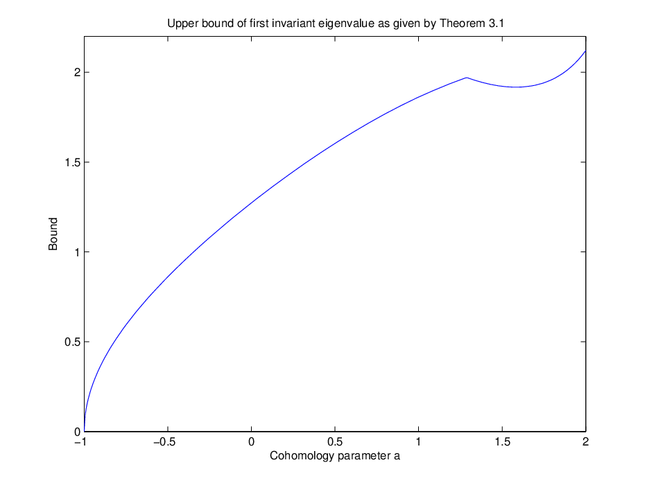
This theorem suggests that for small values of the parameter $a$, it is the $\mathbb{Z}_{2}$-anti-invariant functions that contain the minimising eigenfunction but this switches at some point $a_{c}\approx 1.2877$ and then the invariant functions contain the minimising eigenfunction. We can plot the bound as a function of $a$, the result of this is contained in Figure 1. As we have an explicit form for each extremal metric, we are able to investigate exactly how accurate the bound in Theorem 3.1 is. To do this we use the Rayleigh-Ritz approximation where our set of test functions is

$$T=\{1,x_{1},x_{2},x_{1}^{2},x_{2}^{2},x_{1}x_{2}\}.$$

Labelling $\phi_{1}(x)=x_{1}$, $\phi_{2}(x)=x_{2}$,…, $\phi_{6}(x)=x_{1}x_{2}$, we compute the two $6\times 6$ matrices

$$M_{ij}=\langle\phi_{i},\phi_{j}\rangle_{L^{2}}\textrm{ and }\widetilde{M}_{ij}=\langle\nabla\phi_{i},\nabla\phi_{j}\rangle_{L^{2}}.$$

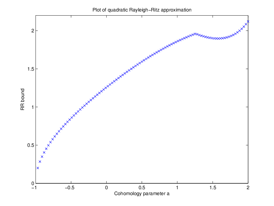
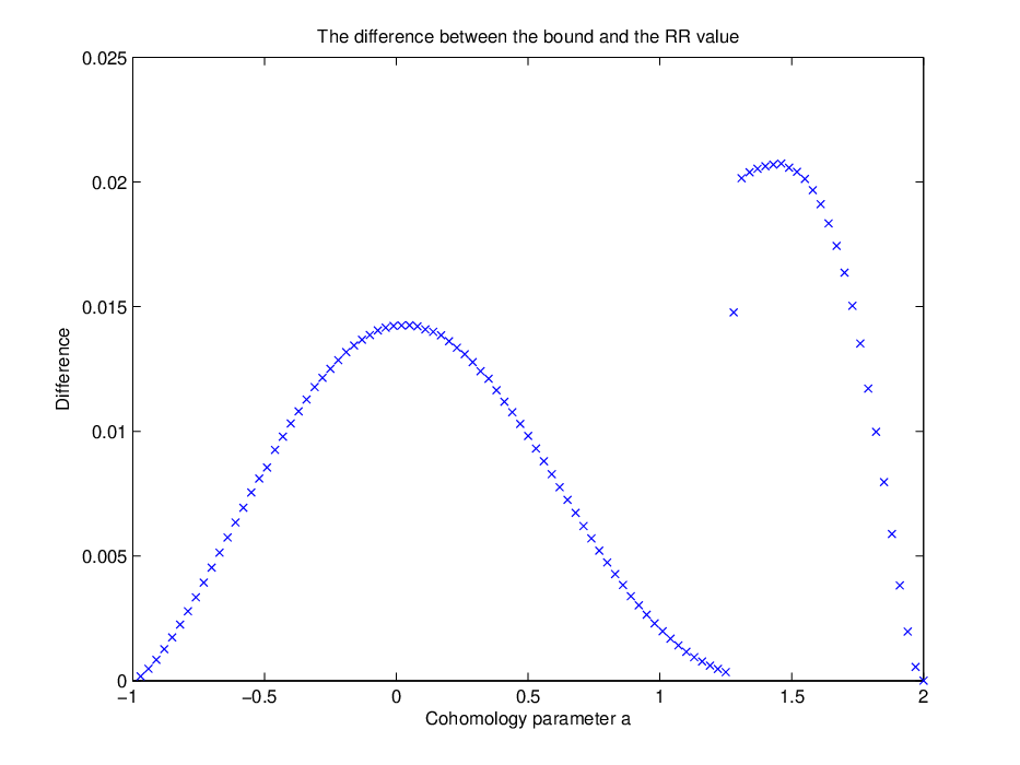
The Rayleigh-Ritz approximation is then given by the smallest positive eigenvalue of the matrix $M^{-1}\widetilde{M}$. We plot this for 100 equally spaced values of $a$ in Figure 2. As the plot shows, the behaviour of this quantity is very similar to that of the upper bound in Theorem 3.1 with the same switching from the smallest eigenfunction being $\mathbb{Z}_{2}$-anti-invariant to $\mathbb{Z}_{2}$-invariant at $a\approx 1.2877$. To show just how close the bound is to this quantity we plot the difference of the bound and the Rayleigh-Ritz approximation in Figure 3.

It is also interesting to note that informally at least, as $a\rightarrow 2$,

$${(\mathbb{C}P^{2}\sharp-\mathbb{C}P^{2},g_{a})\rightarrow(\mathbb{CP}^{2},\gamma g_{FS})}$$

where $\gamma=2\sqrt{2}/3$. It is well-known that $\lambda_{1}=\lambda_{1}^{\mathbb{T}}=2$ for $g_{FS}$ and so we see that the absolute upper bound for $\lambda_{1}^{\mathbb{T}}$ in the family of extremal metrics is that of the rescaled Fubini-Study metric $3\sqrt{2}/2\approx 2.12$. Hence in both the $\mathbb{C}P^{1}\times\mathbb{C}P^{1}$ and ${\mathbb{C}P^{2}\sharp-\mathbb{C}P^{2}}$ cases, the value of $\lambda_{1\mathbb{T}}$ for the one parameter family of extremal metrics is bounded above absolutely by the eigenvalue of the Kähler-Einstein metric in the family.

There are further toric surfaces formed by blowing up points on $\mathbb{C}P^{2}$ which admit extremal metrics as well as higher dimensional examples. One difficulty in studying these manifolds is that the precise existence results are much more difficult to state. For example, not every Kähler class on the surface $\mathbb{C}P^{2}\sharp-2\mathbb{C}P^{2}$ admits an extremal metric. Nevertheless it should be possible to derive analogues of Theorem 3.1 quite easily. Testing the accuracy of the bounds will be more challenging as very few of the metrics are known in a closed form. There are some approaches to numerically approximating such metrics [6] [15] that would allow the calculation of the Rayleigh-Ritz matrices in simple cases. The authors hope to discuss this in separate work.

References

- [1] Abreu M., Kähler geometry of toric varieties and extremal metrics, Internat. J. Math., 9, (1998), 641–651.
- [2] Abreu M., Kähler geometry of toric manifolds in symplectic coordinates, Symplectic and Contact Topology: Interactions and Perspectives. Fields Inst. Commun. 35, 1-–24 (2003) Toronto, ON/Montreal, QC.
- [3] Abreu M., Freitas P., On the invariant spectrum of -invariant metrics on , Proc. London Math. Soc. (3) 84, no. 1, (2002), 213–230.
- [4] Batat W., Hall S. J., Jizany A., Murphy T., Conformally Kähler geometry and quasi-Einstein metrics, preprint (2015), arXiv:1502.07140v1 [math.DG].
- [5] Brion M., Points entiers dans les polyédres convexes, Ann. Sci. École Norm. Sup., 21, no. 4, (1988), 653–-663.
- [6] Bunch R., Donaldson S. K., Numerical approximations to extremal metrics on toric surfaces, Handbook of Geometric Analysis, Adv. Lect. Math., vol. 7(1), (2008), 1–-28.
- [7] Calabi E., Extremal Kähler metrics II. In: Differential Geometry and Complex Analysis, pp. 95–114, Springer, Berlin (1985).
- [8] Delzant T., Hamiltoniens périodiques et images convexes de l’application moment. Bull. Soc. Math. Fr., 116, no. 3, (1988), 315��–339.
- [9] Donaldson S. K., Scalar curvature and stability of toric varieties, J. Diff. Geom., 62 , no. 2, (2002), 289–349.
- [10] Engman M., Trace formulae for -invariant Green’s operators on , Manuscripta Math., 93, no. 3, (1997), 357–368.
- [11] Engman M., The spectrum and isometric embeddings of surfaces of revolution, Canad. Math. Bull., 49, no. 2, (2006), 226–236.
- [12] Guillemin V., Kaehler sturctures on toric varieties, J. Differential Geom. 40, no. 2, (1994), 285–309.
- [13] Hall S. J., Murphy T., On the spectrum of the Page and the Chen-LeBrun-Weber metrics, Ann. Glob. Anal. Geom., 46, no. 1, (2014), 87–101.
- [14] Hall S. J, Murphy T., Bounding for Kähler–Einstein metrics with large symmetry groups, Ann. Glob. Anal. Geom., 46, no. 2, (2014), 145–158.
- [15] Hall S. J., Murphy T., Numerical approximations to extremal toric Kähler metrics with arbitrary Kähler class, preprint (2014), arXiv:1407.1272v1 [math.DG].
- [16] Hersch J., Quatre propriétés isopérimétriques de membranes sphériques homogènes, C. R. Acad. Sci. Paris Sér. A-B, 270, (1970), A1645–A1648.
- [17] Lasserre J. B., Avrachenkov K., The multidimensional version of , Amer. Math. Mon., 108, no. 2, (2001), 151–-154.
- [18] Legendre, E., Sena-Dias, R. Toric aspects of the first eigenvalue, preprint (2015).